1. Introduction
Soil moisture, is an important hydrologic variable that controls the interactions (and feedbacks) between land surface and atmospheric processes [
1]. It plays a very important role in the distribution of precipitation between runoff and infiltration. Soil moisture monitoring and characterization of the spatial and temporal variability of this hydrologic parameter at scales from small catchments to large river basins continues to receive much attention, reflecting its critical role in subsurface-land surface-atmospheric interactions and its importance to drought analysis, crop yield forecasting, irrigation planning, flood protection, and forest fire prevention [
2,
3,
4].
In semi-arid environments ground water recharge is one of the most difficult parameters to quantify, where a number of recharge mechanisms, including soil moisture change, on variable temporal and spatial scales. Several studies showed that temporal analysis of soil moisture can be used to understand ground water recharge [
5,
6]. Remote sensing technology has been used successfully to estimate soil moisture [
3,
7,
8,
9,
10] and map its spatio-temporal distribution in semi-arid environments and could potentially contribute to ground water recharge studies.
Synthetic Aperture Radar (SAR) data are particularly well suited for estimating soil moisture due to the relationship between the dielectric constant and soil moisture [
11,
12]. The microwave measurements are strongly dependent on the dielectric properties of the target. For a soil, dielectric properties are a function of the amount of water present. The real part of the complex dielectric constant of water in this spectral region (microwave) is approximately 80 comparing to the value for dry soil is about three. This large contrast provides a basis for estimating the moisture for dielectric values between these two extremes [
13,
14]. It is not always possible to take advantage of the dielectric constant and soil moisture relationship since microwave measurements are also influenced by surface roughness, which varies significantly from place to place due to diverse land use and land covers. That’s why no global SAR based operational algorithm exists for estimating soil moisture [
15].
Studies, particularly in the past two decades, have resulted in a multitude of methods, algorithms, and models relating satellite-based radar backscatter imagery to estimate surface soil moisture content [
3,
10,
11,
16,
17,
18,
19,
20]. The most commonly used algorithms are developed by a semi-empirical approach [
21,
22]. In a given bare soil condition, radar backscatter is linearly dependent on volumetric soil moisture content (θ
w) in the upper 2 to 5 cm of soil with a correlation (R
2)~ 0.8 to 0.9 [
21,
22]. However, the presence of vegetation cover complicates soil moisture estimation due to the interaction of the microwaves with the vegetation and soil [
12]. The radar backscatter from a surface with vegetation consists of three components: (1) product of the backscatter contribution of bare soil surface (σ
s°) and the two way attenuation of the vegetation layer (τ
2), (2) the direct backscatter contribution of the vegetation layer (σ°
dv), and (3) multiple scattering involving the vegetation elements and the ground surface (σ°
int) [
12].
In soil moisture estimation for semi-arid environments using different SAR data the influence of sparse vegetation were found negligible by several studies [
11,
16,
17,
18,
19,
22]. That means, for a given soil with uniform surface roughness (
R), θ
w can be estimated using the following simple linear regression expression since in this case σ° ≈ σ°
s.
where
a and
b are regression coefficients, usually determined from field experiments encompassing the target-invariant
, scene-invariant SAR wavelength, incidence angle, polarization, and calibration.
Using high resolution SAR data, however, it is not always possible to obtain strong linear relationship between measured soil moisture and radar backscatter even in semi-arid environments. Depending on the amount of vegetation present, its dielectric properties, height and geometry, the sensitivity of microwave backscatter to variations in volumetric soil moisture may be significantly reduced [
23]. As shown by [
23], in a semi-arid environment of south-eastern New Mexico vegetation coverage can significantly reduce the accuracy of soil moisture estimation using numerical models based on simple linear (R
2 = 0.05 to 0.24) and non-linear (R
2 = 0.24) relationships between radar backscatter from high resolution SAR imagery and near real time
in situ soil moisture measurements. In addition to the vegetation density, the SAR backscattering can also be influenced by the variation in soil types and soil salinity since they may affect the surface dielectric properties. Topographic variations can also influence the distribution of soil moisture in the field.
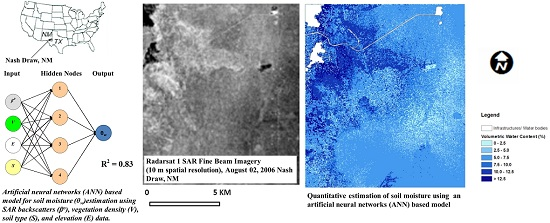
This paper investigated the potential of multiple linear regressions and Artificial Neural Networks (ANN) based models to improve soil moisture estimation in south-eastern New Mexico using high resolution Radarsat 1 SAR imagery. The models used SAR backscatters and near real time soil moisture measurements along with vegetation density, soil type, elevation, and soil salinity measurements. A time series of SAR based soil moisture estimation data were generated for an entire wet season in the study site using the developed numerical models.
2. Study Site
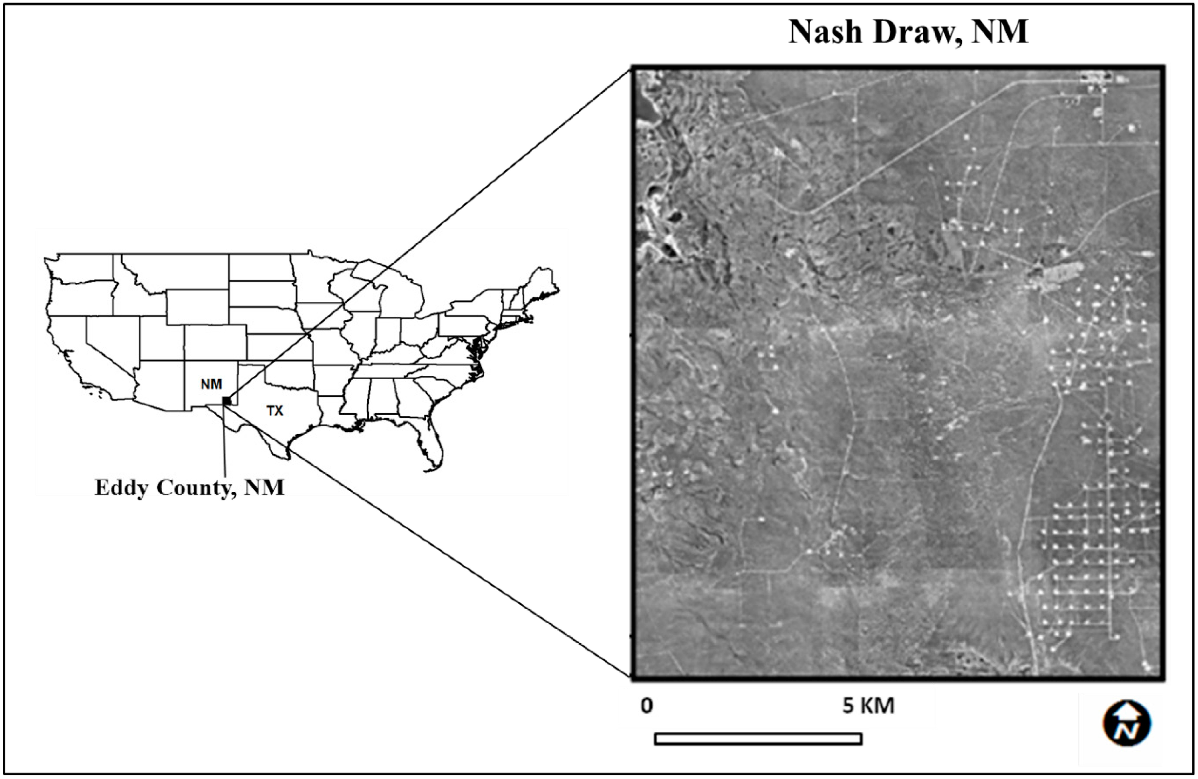
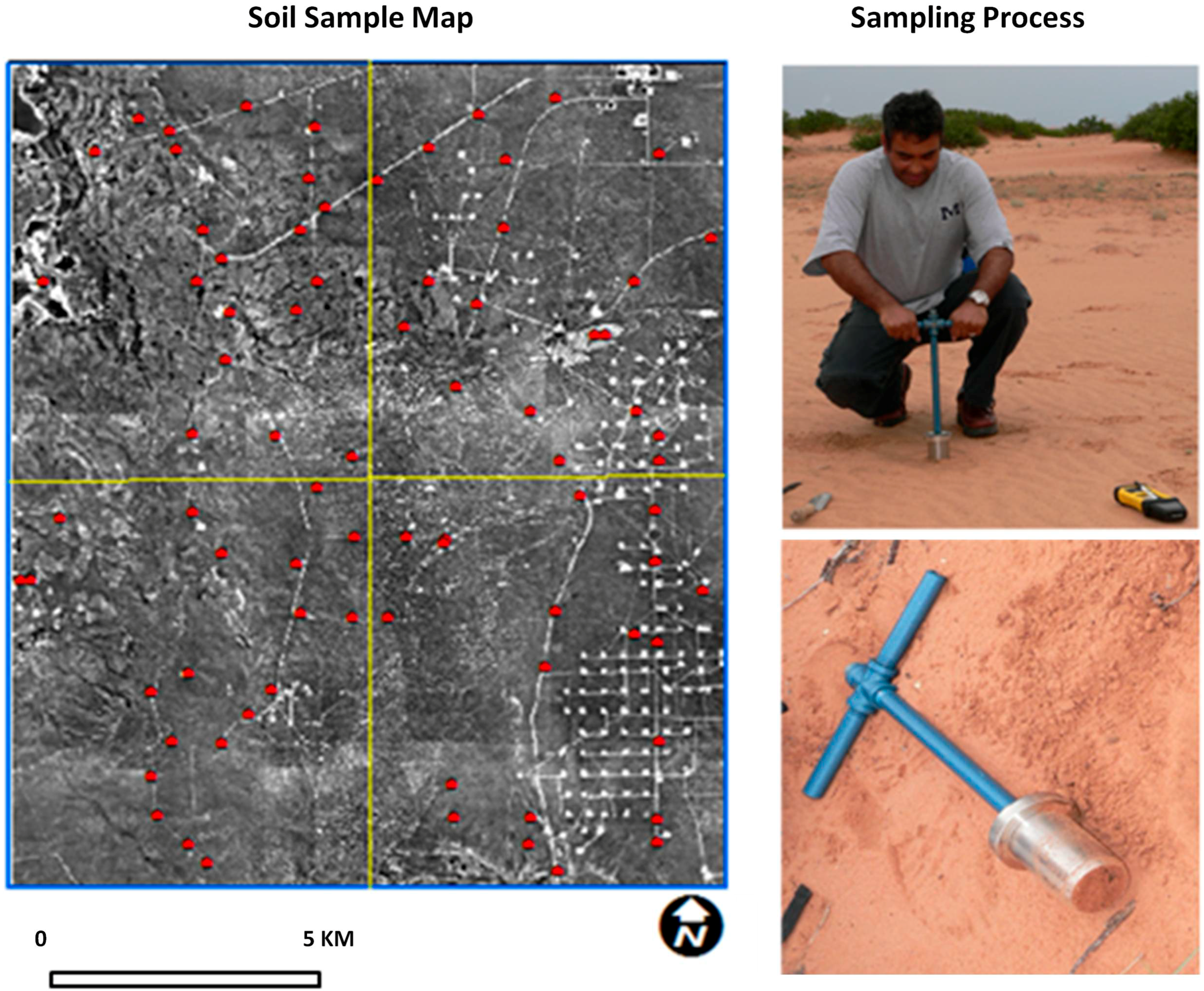
A small area in south-eastern New Mexico called Nash Draw was selected as the study site for this study (
Figure 1). It is located about 30 km east of Carlsbad, NM. It covers an area of about 400 km
2 and the study site occupies 225 km
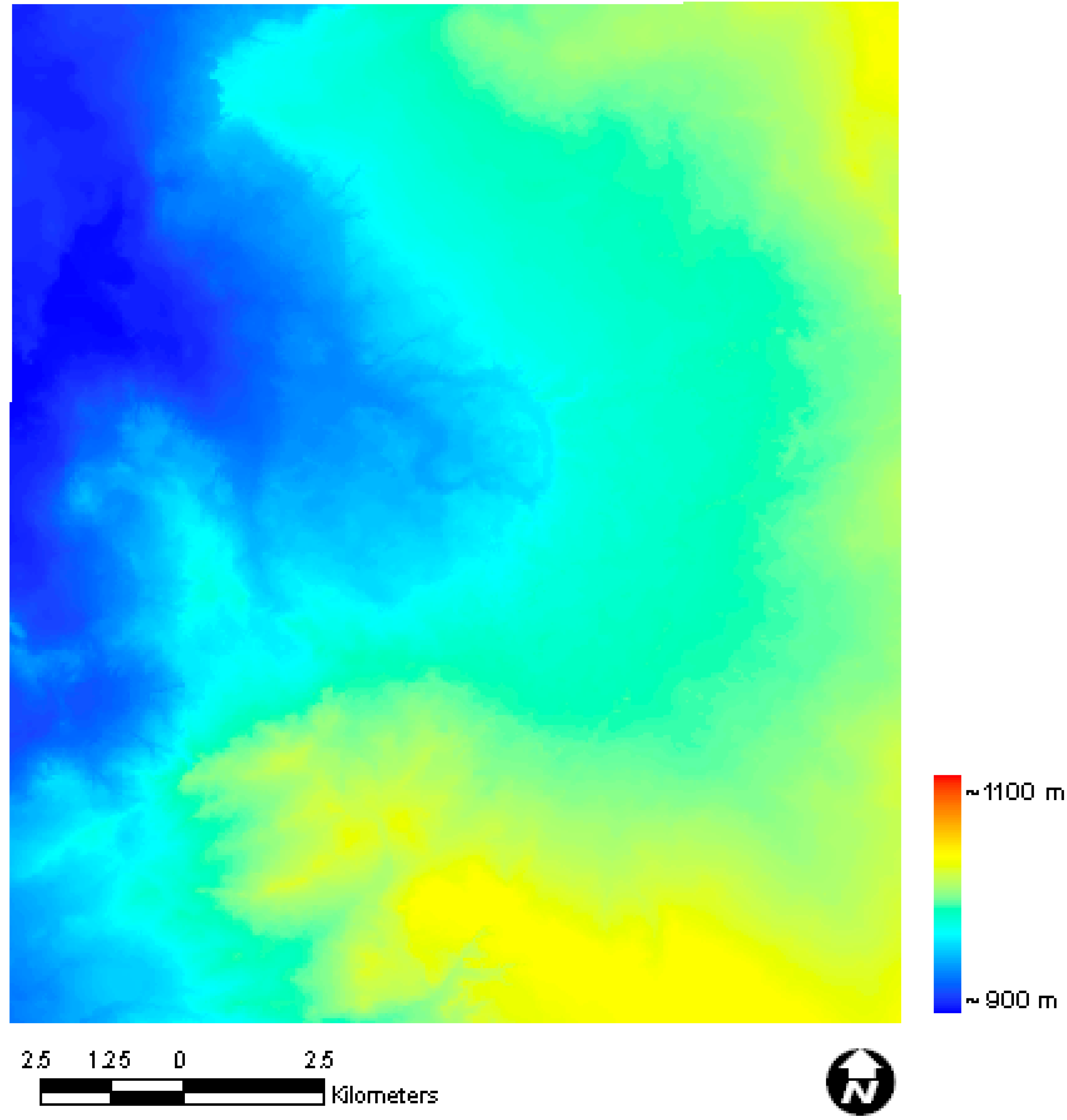
2 of it. The extent of the site is limited between 103.78°W–103.92°W longitude and 32.23°N–32.36°N latitude. It is a part of the north-eastern Chihuahua desert, which is characterized by semi-arid environments and sparsely vegetated rangeland. The topographic relief in the region is not significant. The maximum relief across the area is approximately 200 m.
Nash Draw is a karst valley that developed in response to subsurface dissolution of evaporites (including halite and sulfate rocks) and subsidence of the overlying strata [
24]. It is a complex example of the localized effects of evaporite karst on surface topography, near-surface geology, and hydrology [
25]. Different areas of Nash Draw display small karst features, including caves, sinkholes, dolines, and larger integrated forms such as valleys or elongated depressions [
25].
The hydrologic system within Nash Draw is poorly understood. Much of Nash Draw exhibits no significant integrated surface drainage [
25], while much of the area is covered by a thick blanket of dune sand. That is why it is very difficult to identify the potential locations for ground water recharge in this area. Therefore, to assist in understanding the existing hydrologic processes modifying Nash Draw it is very important to determine the spatio-temporal distribution of surface soil moisture.
Since the study site covers an area of 225 km2 high resolution SAR data would be very suitable to obtain remote sensing derived soil moisture estimation for this area. This is the reason Nash Draw was found suitable as a test site for the conducted study.
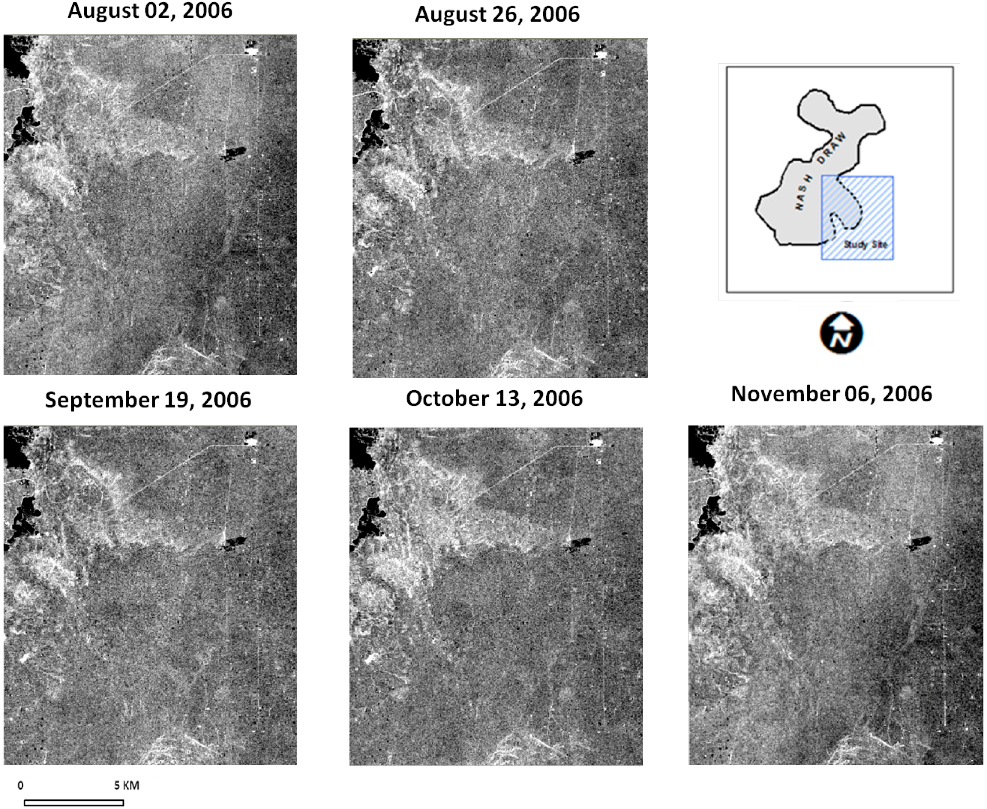
Rainfall in Nash Draw is unreliable and erratic, with August as the wettest part of the year and the rainy season ending in October. Therefore, it was considered that imagery acquired from August to November should record the maximum variation of soil moisture in the study site.
Figure 1.
Location of study site.
Figure 1.
Location of study site.
4. Methods
In this study, multiple linear regressions and Artificial Neural Networks (ANN) based models were used to investigate the influence of vegetation, elevation, soil type, and salinity on soil moisture estimation using microwave imagery. Coefficient of determination (R2) values were used to evaluate the suitability of the different numerical models to estimate and map soil moisture distributions. Soil moisture maps were prepared for the five SAR imagery acquisition dates using the most suitable numerical model.
4.1. Multiple Linear Regressions
In semi-arid environments, the influence of sparse vegetation was found negligible in several soil moisture estimation studies using SAR data, e.g., [
11,
16,
17,
18,
19]. However, as shown by [
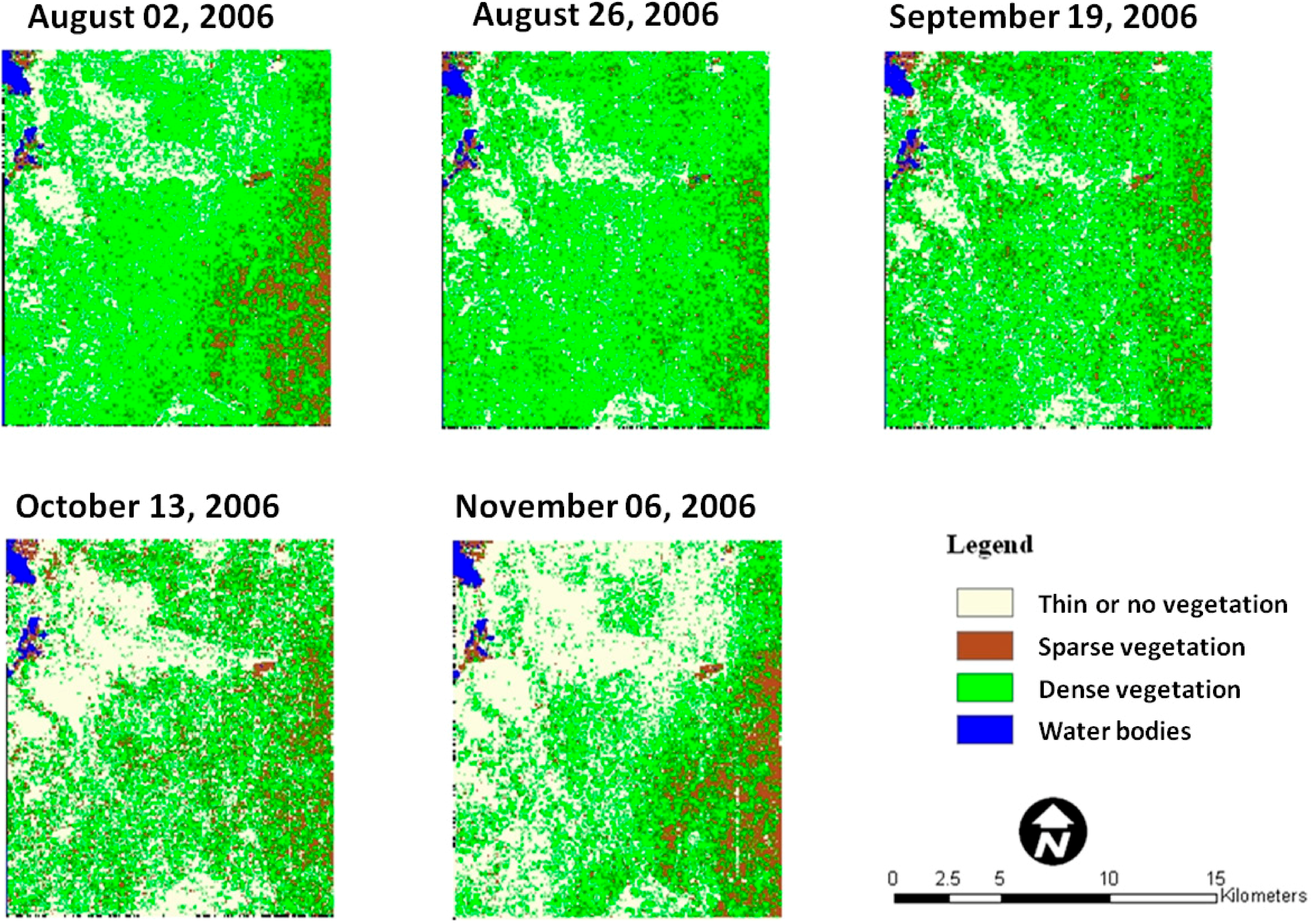
23] the vegetation distribution pattern in Nash Draw could significantly influence the soil moisture estimation using high resolution SAR data. The obtained vegetation density and distribution maps of Nash Draw (
Figure 5) also support this observation.
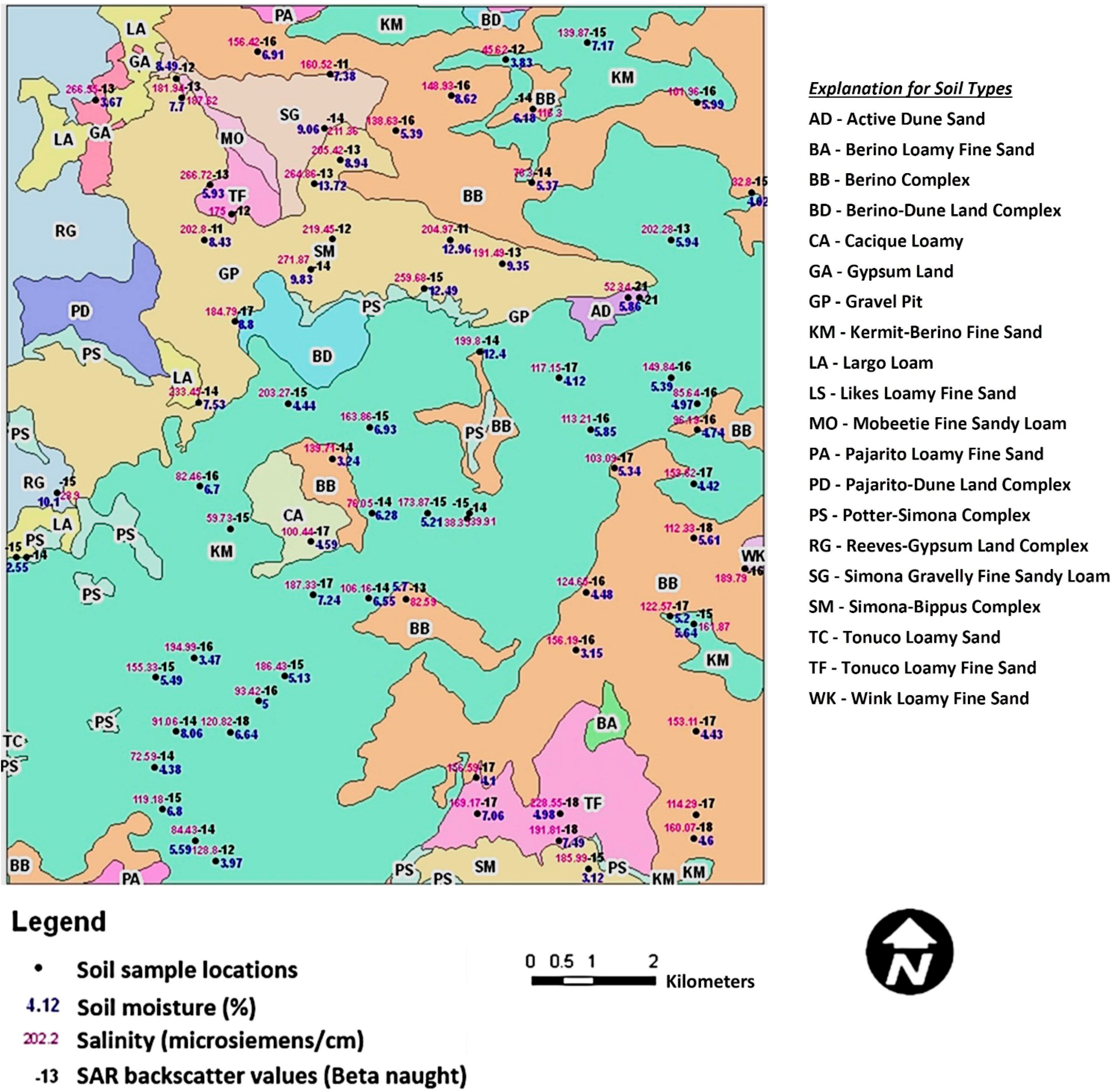
In estimating soil moisture from low frequency radar backscattering (L band radar), the di-electric constant was found to be weakly sensitive to soil types [
12]. The sensitivity of higher frequency radar backscattering (C band radar) to soil types, however, has not been fully analyzed in the published literature. Several studies reported that soil moisture estimation using L-band radar should consider the impact of soil salinity in the model [
36,
37,
38]. Since in this research the soil moisture estimation model used C band radar, the impact of both soil type and soil salinity on soil moisture estimation was investigated.
Multiple linear regressions were conducted incorporating vegetation density information, elevation, soil type, and soil salinity in addition to radar backscattering (measured as βº) to estimate soil moisture in the study site. The regression was done in a step fashion where independent variables (vegetation density information, elevation, soil type, and soil salinity) were sequentially added to the regression analysis to evaluate the effects of each independent variable in soil moisture estimation.
Equations (7)–(11) are the numerical models developed by multiple linear regressions with the observed
in situ soil moisture measurements and different combination of independent variables to estimate soil moisture in Nash Draw, NM. The observed soil moisture data were acquired from the 2 August data set.
Table 2 shows the coefficient of determination (R
2) values of the corresponding models. From the results of the simple linear regressions it was found that both the 2 August and the 6 November data sets produced similar results. Therefore, it was decided to use only one data set to evaluate the model performance.
where, β°—Backscatter value,
V—Vegetation,
S—Soil type,
E—Elevation, and
SL—Soil salinity.
Table 2.
Coefficient of determination (R2) values of multiple linear regression based models.
Table 2.
Coefficient of determination (R2) values of multiple linear regression based models.
| Independent Variables | Coefficient of Determination (R2) | Insignificant Variables |
|---|
| β°, V | 0.50 | -- |
| β°, V, S | 0.60 | -- |
| β°, V, E | 0.51 | E |
| β°, V, S, E | 0.61 | E |
| β°, V, S, E and SL | 0.66 | E and SL |
4.2. Artificial Neural Networks (ANN)
Most SAR based soil moisture estimation models are based on the assumption that soil moisture distribution is linearly related to the radar backscatter of the soil moisture surface, e.g., [
11,
12,
21,
39]. There are a few studies that explore the non-linear relationships between soil surface moisture and radar backscatters. In this study, Artificial Neural Networks (ANN) based numerical models were developed to estimate soil surface moisture from SAR data and to explore the non-linear relationship between soil moisture and SAR backscatters. The significance of vegetation coverage, elevation, soil type, and soil salinity in soil moisture estimation using SAR data and artificial neural networks based models was also investigated.
Artificial neural networks, are a branch of artificial intelligence [
40] in which the solution to a problem is learned from a set of examples [
41]. A neural network can be regarded as a nonlinear mathematical function, which transforms a set of input variables into a set of output variables. The use of neural networks has been shown to be effective alternatives to more traditional statistical techniques [
42]. Neural networks can be trained to approximate any smooth, measurable function [
42], can model highly non-linear functions, and can be trained to be accurately generalized when presented with unseen data [
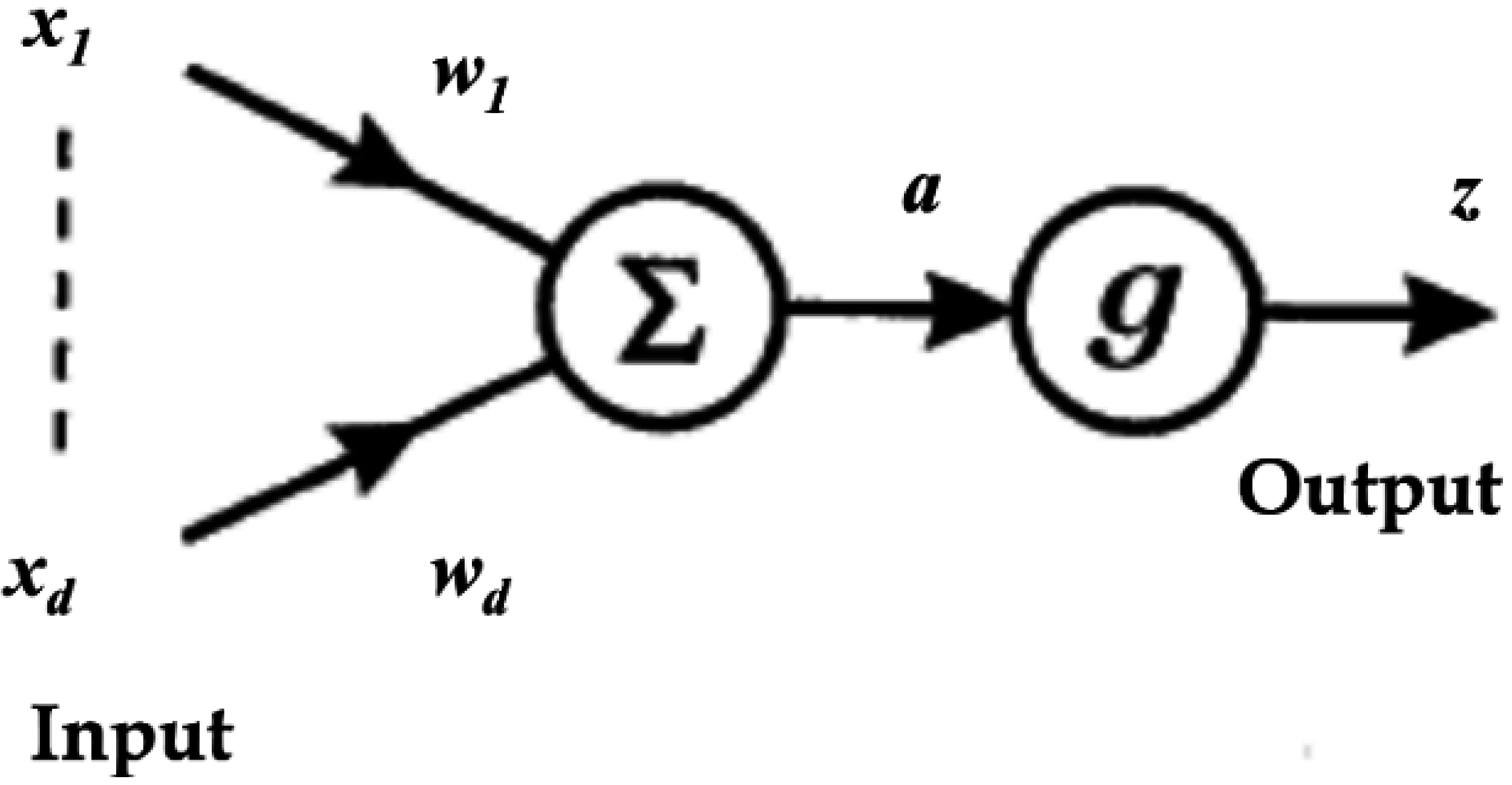
26]. In a typical neural network model, a single neuron forms a weighted sum of the inputs
x1,x2,…,xd given by
a = Σiwixi, and then transforms this sum using a non-linear activation function
g( ) to give a final output
z =
g(a) (
Figure 7).
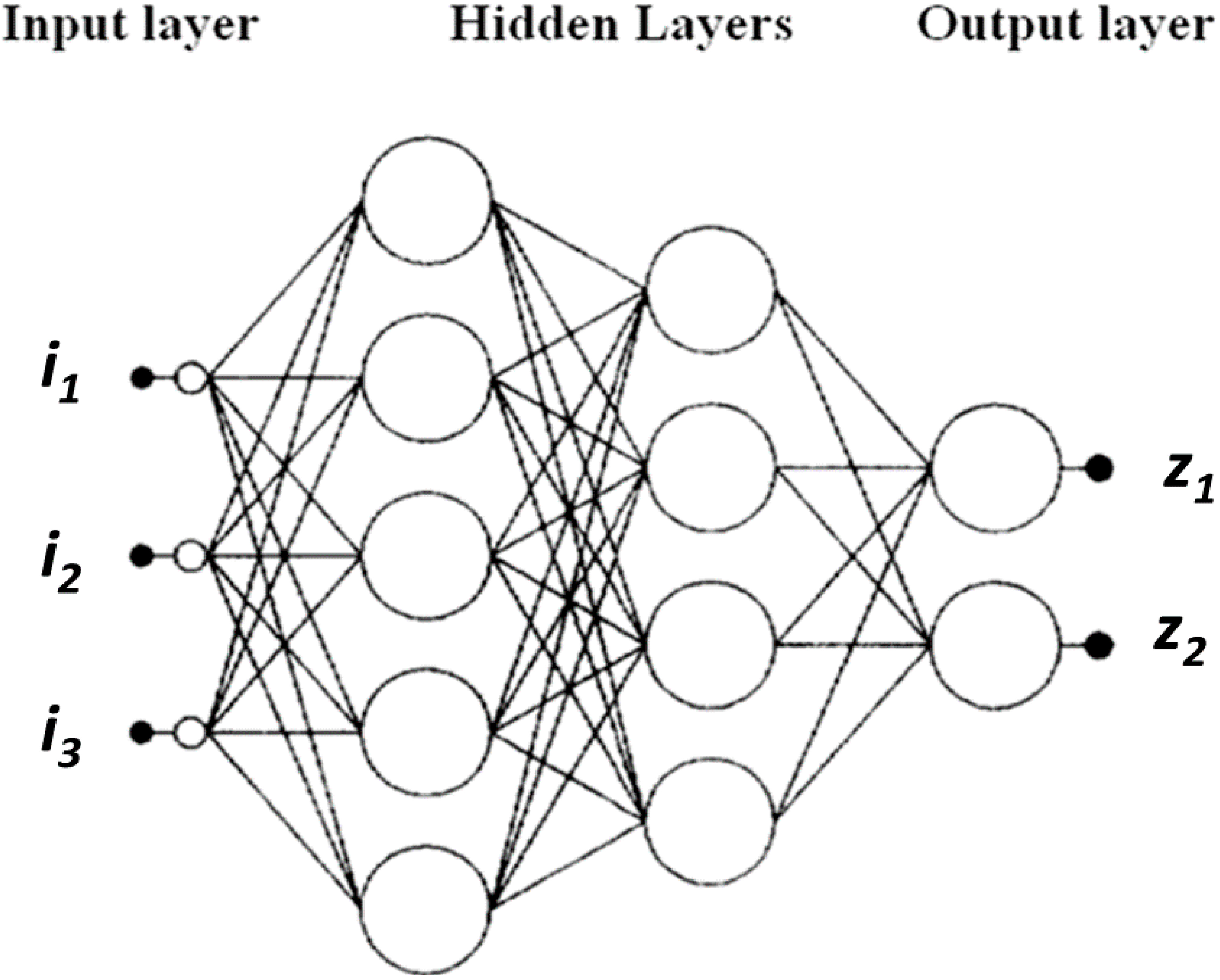
A feed forward neural network can be regarded as a nonlinear mathematical function, which transforms a set of input variables into a set of output variables. The multilayer perceptron is the most widely used feed forward neural network.
Figure 7 shows a single processing unit of neural networks. If we consider a set of
m such units, all with common inputs, then we arrive at a neural network having a single layer of adaptive parameters (weights) as illustrated in
Figure 8. The output variables are denoted by
zj and are given by Equation (12).
where
wji—the weight from input
i to unit
j, and
g( )—an activation function as discussed previously.
Figure 7.
A single processing unit in neural networks.
Figure 7.
A single processing unit in neural networks.
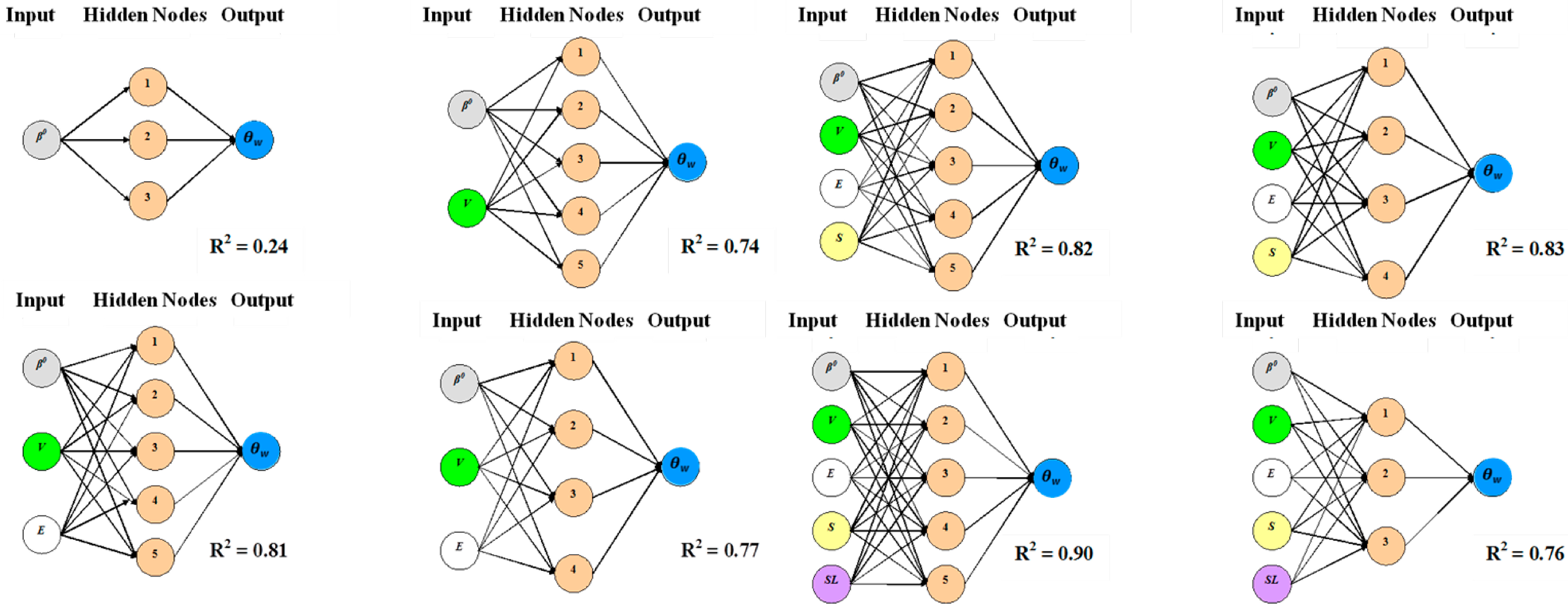
Artificial neural networks, based non-linear numerical models were developed for soil moisture estimation for the entire study site using the 2 August data set. Five different neural networks based models were developed, through addition of different variables, to estimate soil moisture in Nash Draw. The first model had only one input, the backscatter values. This model uses the non-linear relationship between radar backscatter and soil moisture content. The other four models used additional inputs (e.g., vegetation coverage, elevation, soil type, and soil salinity) in different combinations with radar backscatter values. JMP statistical software was used to perform the neural networks based analysis. The model coefficient of determination (R
2) and cross validation coefficient of determination (CV R
2) values were used to evaluate the model performance for soil moisture prediction. The impact of soil salinity was investigated and inclusion of this variable did not significantly improve model performance.
Figure 9 shows the simplified schematic of the models that were developed.
Table 3 shows the R
2 and CV R
2 values of the corresponding models.
Figure 8.
A multilayer perceptron with two hidden layers.
Figure 8.
A multilayer perceptron with two hidden layers.
Figure 9.
Neural networks based numerical models for soil moisture estimation in Nash Draw, NM, USA. Note: β°—Backscatter value; V—Vegetation; S—Soil type; E—Elevation; SL—Soil salinity.
Figure 9.
Neural networks based numerical models for soil moisture estimation in Nash Draw, NM, USA. Note: β°—Backscatter value; V—Vegetation; S—Soil type; E—Elevation; SL—Soil salinity.
Table 3.
Coefficient of determination (R2) and cross validation coefficient of determination (CV R2) of the neural networks based numerical models for soil moisture estimation.
Table 3.
Coefficient of determination (R2) and cross validation coefficient of determination (CV R2) of the neural networks based numerical models for soil moisture estimation.
| Input Variables | Hidden Nodes | Coefficient of Determination (R2) | Cross Validation (CV) R2 |
|---|
| β° | 3 | 0.24 | 0.11 |
| β°, V | 5 | 0.74 | 0.49 |
| β°, V, E | 4 | 0.77 | 0.54 |
| β°, V, E | 5 | 0.81 | 0.44 |
| β°, V, E, S | 4 | 0.83 | 0.56 |
| β°, V, E, S | 5 | 0.82 | 0.47 |
| β°, V, E, S and SL | 3 | 0.76 | 0.45 |
| β°, V, E, S and SL | 4 | 0.82 | 0.54 |
| β°, V, E, S and SL | 5 | 0.90 | 0.58 |
5. Results
5.1. Soil Moisture Estimation
Near-real time field observations, acquired at the beginning and end of the time series, in conjunction with SAR data were used to estimate soil moisture from the SAR imagery acquired on five different dates in 2006. Model coefficient of determination (R2) and model cross validation coefficient of determination (CV R2) (for non-linear models) values were compared and used to evaluate their suitability for soil moisture estimation in Nash Draw. The model with the highest R2 and CV R2 values was considered as the most appropriate model for soil moisture estimation. The accuracy of the selected models was evaluated by Kappa statistics. The selected soil moisture estimation numerical models were then used to convert ߺ SAR data into soil moisture data. The soil moisture data was divided into several categories to aid in the interpretation of the spatial distribution of the soil moisture in the study site.
The following observations were made after the evaluation of the R
2 and CV R
2 values of the models developed for soil moisture estimation in Nash Draw, NM.
Simple linear regression between radar backscatter values and
in situ soil moisture measurements can be used to develop SAR-based soil moisture estimation models with model R
2 values of 0.51 to 0.61, but application of the model should be restricted to non-vegetated to thinly vegetated areas [
23].
Multiple linear regressions using radar backscatter values, vegetation density, soil type, and elevation as independent variables can be used to develop soil moisture estimation models for the entire study site, including areas with thicker vegetation.
Neural networks based models, using radar backscatter values, vegetation density, soil type, and elevation can also be used to estimate soil moisture for the entire study site, including areas with thicker vegetation. Neural networks based models achieved higher R2 values and performed better than multiple linear regressions based models.
A neural network based numerical model using radar backscatter values, vegetation density, soil type and elevation was used to estimate soil moisture in the study site. This model was developed for both the 2 August and the 6 November data sets. The R2 and CV R2 values for the August model were 0.83 and 0.56 respectively, and 0.81 and 0.55 for the November model, respectively.
The model developed for the 2 August data set was also used to map soil moisture for the 26 August data set. The model developed for the 6 November data set was also used to map soil moisture for the 13 October data set. Since 19 September is approximately temporally equal from both 2 August and 6 November, we applied both the 2 August and the 6 November models to the 19 September data set and estimated soil moisture by taking the average of the two estimations.
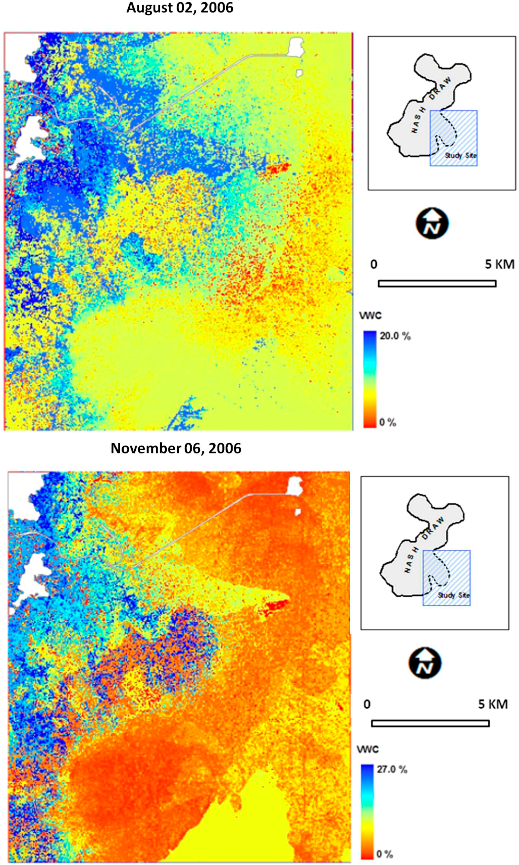
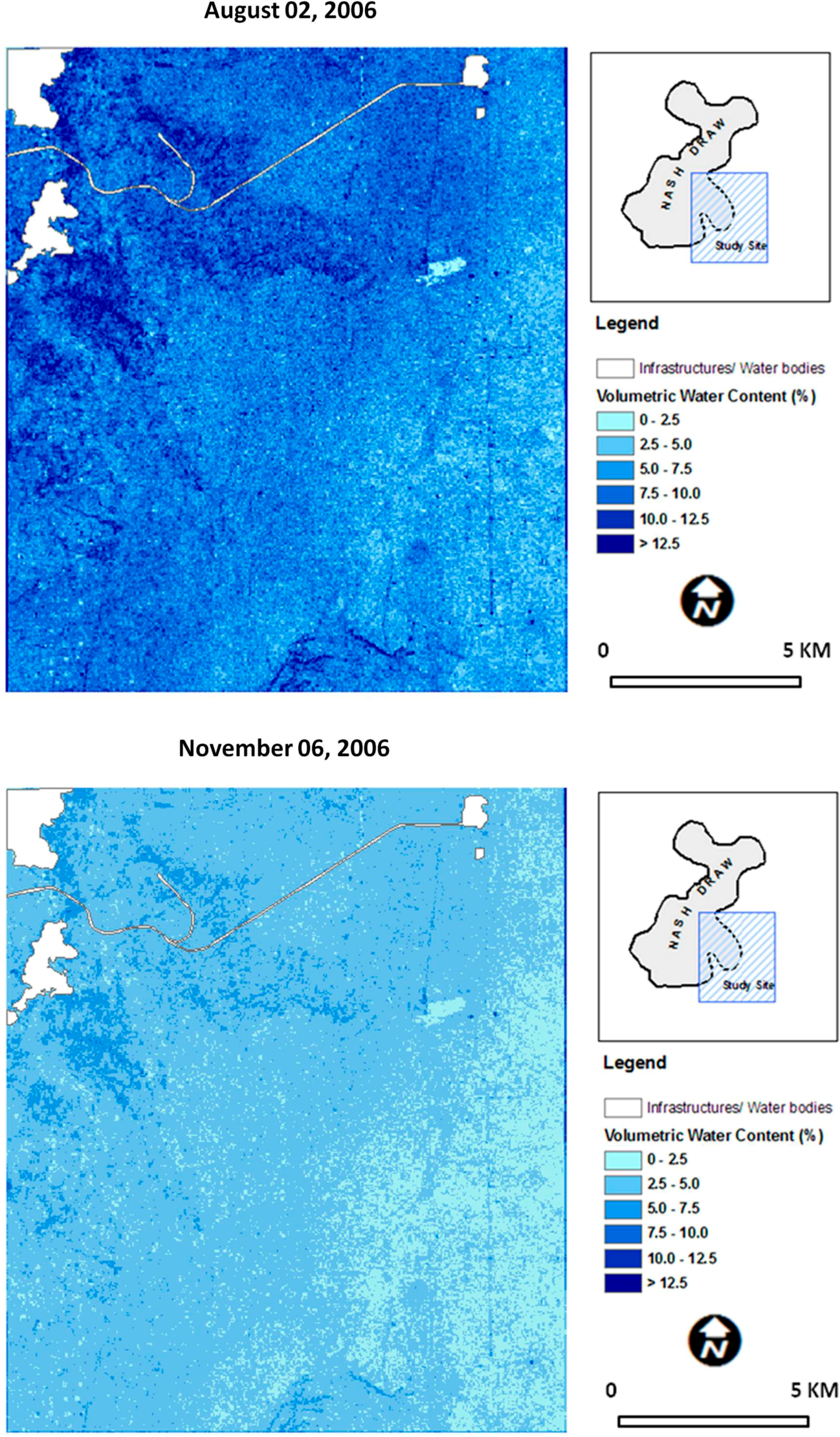
Two sets of 50 m resolution soil moisture data were produced for each of the five dates of SAR data for the study site. The first set includes the unclassified soil moisture data, where the value of each pixel of the dataset is the volumetric soil moisture estimation (
Figure 10). In the second dataset each pixel is classified into six categories of soil moisture to map the spatial variations in soil moisture at 2.5% intervals (
Figure 11).
Figure 10.
Unclassified soil moisture data generated for the study site.
Figure 10.
Unclassified soil moisture data generated for the study site.
Figure 11.
Classified soil moisture data generated for the study site.
Figure 11.
Classified soil moisture data generated for the study site.
5.2. Accuracy Assessment
Kappa statistics [
43,
44] were used to evaluate the accuracy of the soil moisture estimation data produced from the SAR imagery. Kappa statistics have been used successfully for accuracy assessment in different remote sensing based studies, e.g., [
13,
45,
46,
47]. It is a discrete multivariate technique of accuracy assessment [
28]. Kappa coefficients express the proportionate reduction in error generated by a classification process compared with the error of a completely random classification. For example, a value of 0.82 implies that the classification process is avoiding 82% of the errors that a completely random classification generates [
43]. Kappa can be thought of as the chance-corrected proportional agreement, and possible values range from +1 (perfect agreement) to −1 (complete disagreement). A value of 0 indicates no agreement above that expected by chance. The calculation of the Kappa coefficients is explained below using an example of a 2 × 2 matrix (
Table 4).
Table 4.
Computation of Kappa coefficients.
Table 4.
Computation of Kappa coefficients.
| -- | SAR Soil Moisture | Total |
|---|
| Class 1 | Class 2 |
|---|
| Reference Soil Moisture | Class 1 | P11 | P12 | P11 + P12 = α |
| Class 2 | P21 | P22 | P21 + P22 = β |
| Total | P11 + P21 = γ | P12 + P22 = δ | P11 + P22 = χ |
| Total number of data points: Q = α + β = γ + δ |
Observed agreement:
Chance agreement:
Kappa coefficient:
Kappa analysis requires continuous ground truth data so that a sufficient amount of random reference data can be obtained. Therefore, a continuous soil moisture surface was created from the
in situ soil moisture data, using kriging [
48]. Jackknife resampling techniques was used to correct for bias [
49]. The measured
in situ soil moisture data were randomly divided into a training set (90%) and testing set (10%) and were analyzed using the Arc GIS Geostatistical Analyst software. The training data set was used to create the krigged soil moisture surface and the testing data was used to evaluate the kriging results. Ten different krigged soil moisture data sets were generated using 10 different training data sets obtained from the same
in situ soil moisture measurements. The RMS error, average standard error, standardized mean of error, and standardized RMS error (obtained from the evaluation of kriging results with the testing data) were used to select the appropriate kriging surface.
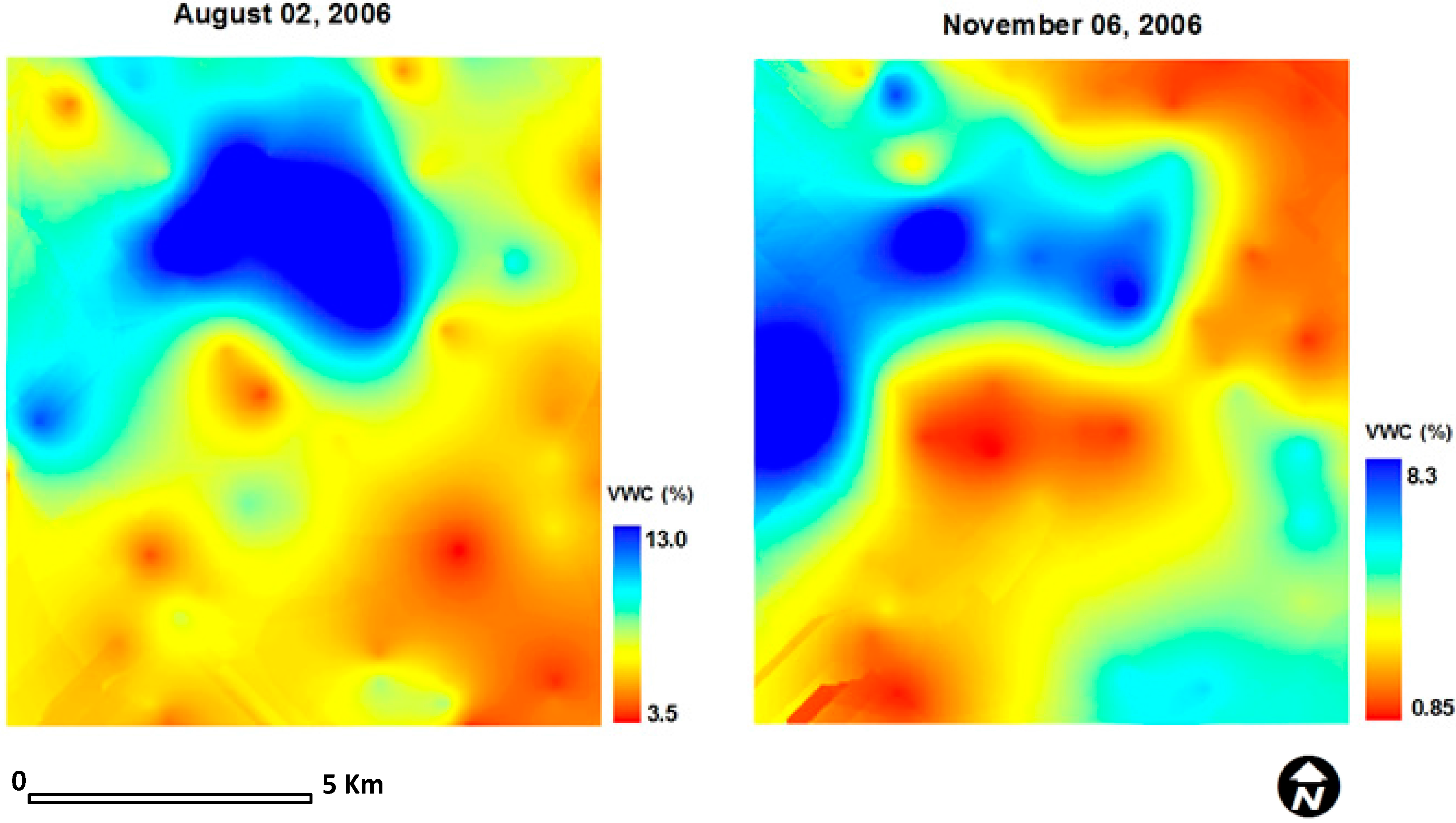
Figure 12 shows the krigged surface generated for the 2 August and 6 November data sets.
Both SAR derived soil moisture data and the krigged soil moisture prediction surfaces were categorized into three class intervals. For the 2 August data set, the classes were 0.0%–5.0%, 5.0%–10.0%, and >10.0%. Since the soil moisture values were much lower in the November data set, these ranges were 0.0%–2.5%, 2.5%–5.0%, and >5.0%. Three hundred randomly generated points were used to calculate the Kappa coefficients and perform an accuracy assessment. Erdas Imagine image processing software was used to perform this accuracy assessment and Kappa analysis. Kappa coefficients were calculated for both the individual classes and the whole data sets.
Figure 12.
Krigged soil moisture surface generation for 2 August and 6 November 2006 field data field data.
Figure 12.
Krigged soil moisture surface generation for 2 August and 6 November 2006 field data field data.
The overall Kappa coefficients obtained for the 2 August and the 6 November data sets were 0.43 and 0.61, respectively. The overall accuracy was 75.67% and 77.67% for the 2 August and the 6 November data sets, respectively.
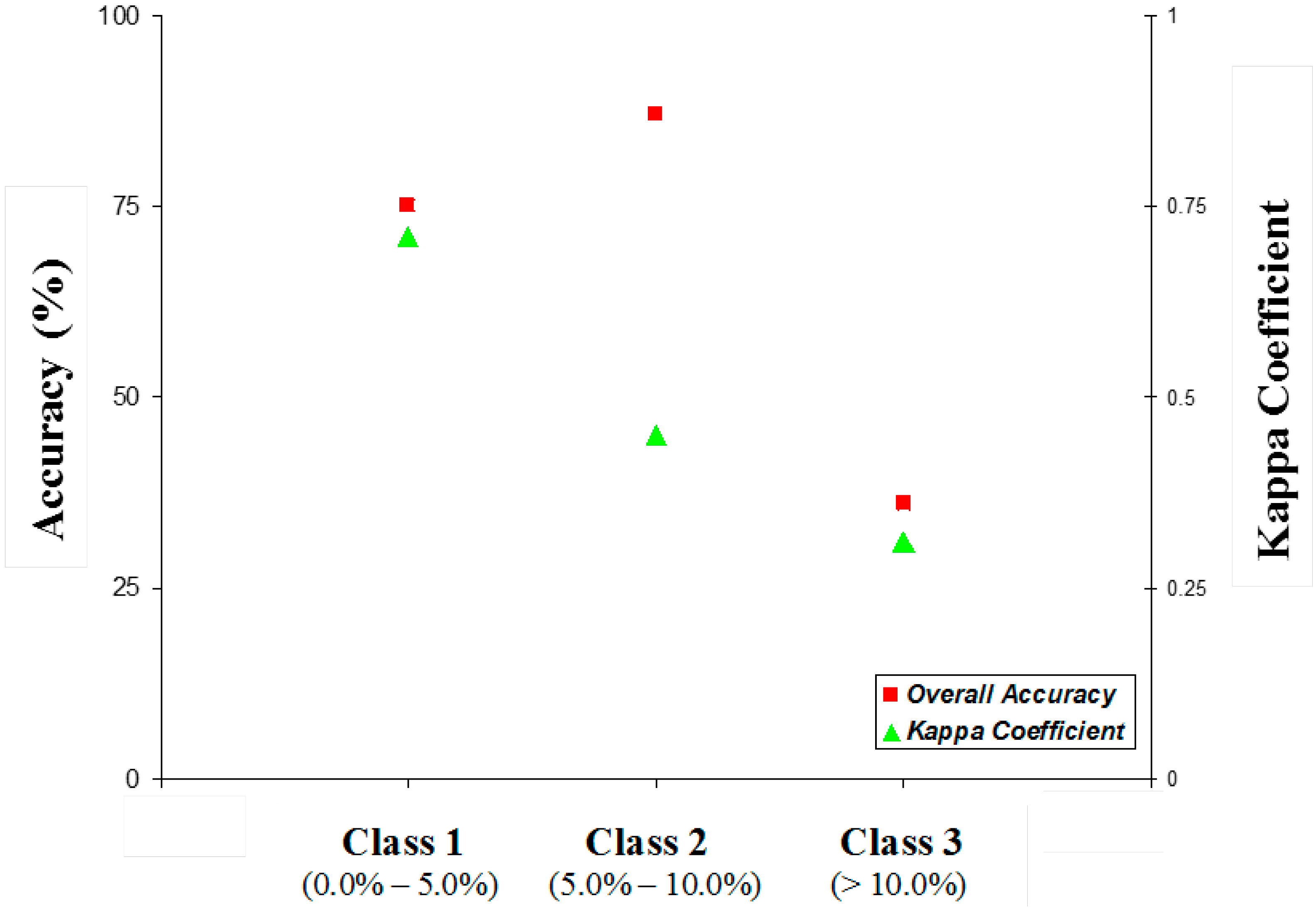
Figure 13 and
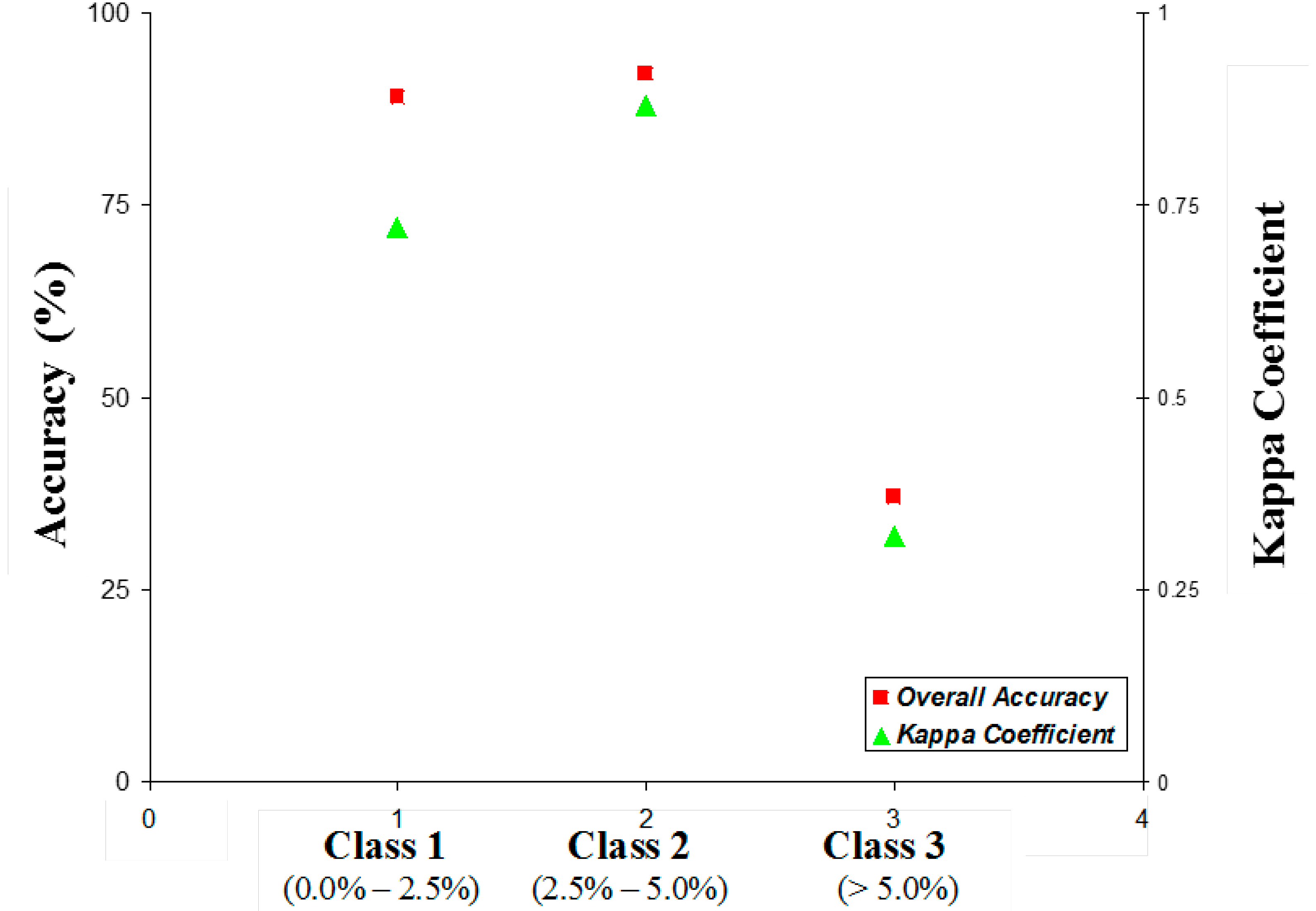
Figure 14 show the Kappa coefficients and classification accuracy for the individual classes. The evaluation of the individual classes indicate that the developed model performed well at low soil moisture regimes compared to the high soil moisture regimes in both 2 August and 6 November data sets.
Figure 13.
Kappa statistics for 2 August 2006 data set.
Figure 13.
Kappa statistics for 2 August 2006 data set.
Figure 14.
Kappa statistics for 6 November 2006 data set.
Figure 14.
Kappa statistics for 6 November 2006 data set.
6. Discussions
Research conducted by [
23] has shown that in semi-arid environments even sparse vegetation can adversely influence the accuracy of soil moisture values estimated from radar backscatter (obtained from high resolution SAR data) using a linear relationship. This observation is supported by lower R
2 values (0.24 and 0.05 for the August and the November datasets respectively) for the linear numerical models developed for the entire study site and higher R
2 values (0.61 and 0.52 for the August and the November datasets respectively) for linear numerical models developed for portions of the study site with little or no vegetation. The lowest R
2 values were from linear numerical models developed for the more densely vegetated portions of the study site (0.01 to 0.04).
This research shows that soil moisture estimation using high resolution SAR data in a semi-arid environment can be improved by developing numerical models that use multiple linear regressions incorporating additional variables such as, vegetation density, soil type, and elevation in addition to radar backscatter values. Regression coefficients as high as 0.61 were obtained for a numerical model covering the entire study site using multiple linear regressions.
The non-linear relationship between radar backscatter values and soil moisture was also investigated by [
23] using artificial neural networks. It showed that a neural network developed using only radar backscatter values and soil moisture had an R
2 value of 0.24, similar to the R
2 value obtained from numerical models using simple linear regressions. This study obtained significant improvement in soil moisture estimation when additional variables such as, vegetation density, soil type, and elevation were added as inputs to the artificial neural networks based models. The use of these additional inputs results in coefficients of determination of 0.83 and 0.81 for the entire study site for the 2 August and the 6 November datasets, respectively. The cross validation coefficients of determination (CV R
2) of the same models were 0.56 and 0.55, respectively.
Soil moisture data were produced using artificial neural networks based non-linear models that incorporated inputs of vegetation density, soil type, elevation, and radar backscatter values. The accuracy of the modeled soil moisture data was also evaluated by the comparison of a soil moisture distribution surface from the models with a soil moisture surface obtained by kriging the
in situ measurements. The comparison was done by Kappa statistics. The overall accuracy and the Kappa coefficient for the soil moisture data obtained for 2 August and 6 November were 75.67% and 77.67%, and 0.43 and 0.61, respectively. Although the obtained kappa coefficient values indicate overall good agreement between the measured and estimated soil moisture values, however, it is worth looking into the possibility of having the influence of autocorrelation between these two soil moisture data sets. As suggested by [
50] since most thematic maps have some degrees of spatial autocorrelation, the calculated expected agreement (by Kappa statistics) could be usually higher than the true expected agreement.
7. Conclusions and Future Work
This research demonstrates the proof of concept of the application of Artificial Neural Networks (ANN) based models for estimating soil surface moisture in semi-arid environments of south-eastern New Mexico using high resolution SAR data (Radarsat 1 SAR Fine data). It is strongly believed that the methods developed in this research can be used to produce soil moisture data from high resolution SAR imagery in semi-arid environments, such as Nash Draw in New Mexico. The hydrology of Nash Draw in New Mexico is characterized by evaporite karst and is not well understood. The data produced in this research should be very useful to identify the pattern of soil moisture distribution in space and time and contribute to a better understanding of the groundwater recharge in the study area.
In the future, to develop an operational soil moisture estimation tool (for this particular area) using high resolution SAR data, the proposed modeling effort can be further enhanced/improved by considering: (1) inclusion of surface roughness parameters in the artificial neural networks based models in addition to vegetation density, soil type, and elevation; (2) incorporation of near real-time high resolution optical satellite data for mapping vegetation density; and (3) involving other statistical tests such as Root Mean Squared Error (RMSE), Mean Absolute Percent Error (MAPE) etc. for model accuracy assessments. It is also recommended to use high resolution l-band SAR data with the capability of multi-polarization. L band data will provide the opportunity to obtain moisture estimation in greater depth.


