On Contraction of Three-Dimensional Multiple Shear Mechanism Model for Evaluation of Large Scale Liquefaction Using High Performance Computing

Abstract

For more reliable evaluation of liquefaction, an analysis model of higher fidelity should be used even though it requires more numerical computation. We developed a parallel finite element method (FEM), implemented with the non-linear multiple shear mechanism model. A bottleneck experienced when implementing the model is the use of vast amounts of CPU memory for material state parameters. We succeeded in drastically reducing the computation requirements of the model by suitably approximating the formulation of the model. An analysis model of high fidelity was constructed for a soil-structure system, and the model was analyzed by using the developed parallel FEM on a parallel computer. The amount of required CPU memory was reduced. The computation time was reduced as well, and the practical applicability of the developed parallel FEM is demonstrated.

1. Introduction

After the accident at the Fukushima Daiichi Nuclear Power station, Japanese electric companies are required to reexamine the seismic safety of existing nuclear power plants in order to continue operation. In these safety reviews, the designed earthquake ground motions, which are much stronger than those used in the initial safety reviews, are used to confirm the earthquake-resistance performance. When a strong ground motion acts on the foundation of a nuclear power plant, soil near the surface behaves in a nonlinear manner, which may result in liquefaction. Therefore, an effective stress analysis method to evaluate the possibility of liquefaction occurrence is usually used in the current licensing work in Japan.

The finite element method (FEM) is a common tool for seismic design, which is especially used for important structures, such as nuclear power plants, that require superior seismic resistance. In general, three-dimensional (3D) is better than the two-dimensional (2D) FEM analysis in order to accurately examine seismic responses of structures. However, 3D FEM analysis is rarely used in practice, since it is time-consuming and requires large amounts of CPU memory.

Effects of soil non-linearity on seismic responses must be more accurately computed when stronger designed ground motion is considered. To this end, a high-fidelity analysis model should be analyzed by FEM. The need for a high-fidelity model increases for the evaluation of liquefaction, since it is a complicated coupling phenomena of soil and underground water. Yamashita et al. [1] and Miyamura et al. [2] reported that an analysis model with sufficiently fine mesh of solid elements can accurately reproduce both local damage and overall response when a non-linear constitutive relationship is implemented. Considering their achievements, we expected that the spatial resolution of liquefaction behavior could be improved by using a high-fidelity analysis model. FEM of a high-fidelity model involves large-scale numerical computation, and a high speed solver (that solves a matrix equation of FEM) is needed for finite element analysis. In this study, we employed FrontISTR [3] as a platform for FEM. This platform has a parallel high-speed solver that is based on the conjugate gradient (CG) method with domain decomposition techniques. It is able to take advantage of various high performance computing (HPC) hardware and software.

We are developing a parallel FEM by implementing tensorial non-linear concrete constitutive relations into FrontISTR for seismic response analysis of reinforced concrete structures. We are implementing tensorial non-linear soil constitutive relations based on the multiple shear mechanism model [4,5,6] and the excess pore water pressure model [7] in order to accurately and efficiently simulate the behavior of soil under liquefaction, to create an analysis model of high fidelity. The multiple shear mechanism model was expanded into 3D by Iai [8], and this formulation was incorporated with various kinds of failure criteria [9]. However, limited results of applying the 3D multiple shear mechanism model have been published. A bottleneck lies in the application of this model occurs due to the requirement of vast amounts of CPU memory to store material parameters, which increases drastically for the 3D setting. We wanted to develop an alternative formulation of the multiple shear mechanism model and to reduce the amount of CPU memory, so that three-dimensional analysis can be easily performed. Hereafter, due to space limitation, the three-dimensional multiple shear mechanism model proposed by Iai is referred to as ‘the original model’ and the three-dimensional multiple shear mechanism model modified by authors as ‘the proposed model’ in this paper.

We studied the usability of the developed FEM for the evaluation of liquefaction. First, the developed 3D multiple shear mechanism model is studied, and then we show that the proposed model depicts non-linear soil behavior similar to the original model, and the required memory is reduced drastically. Next, a high-fidelity analysis model of soil and a structure is analyzed using the developed FEM to confirm the amount by which the memory requirement is reduced and if the proposed model can calculate the same results as the original model. Finally, the scalability of the computational process is studied to demonstrate that the developed FEM has high scalability by using HPC and its execution time required for a given analysis model can be estimated prior to a simulation.

2. Development of Non-Linear Constitutive Relation Based on Multiple Shear Mechanism

2.1. Overview of Past Studies

In the multiple shear mechanism model, a circle placed in three-dimensional space and its center point are considered. In this model, the center point and all the points on the circumference are each connected by a nonlinear spring, and the sum of the force and displacement of the nonlinear spring represent the stress and strain, respectively, at the center point. Each nonlinear spring’s displacement-force relationship follows hyperbolic function, and its displacement and force correspond to its shear strain component and shear stress component in the direction of the spring. The multiple shear mechanism model was originally developed for a 2D model, which uses a circle created on a plane, and this model has already been extended to a 3D model by considering the various planes in three-dimensional space (the original model).

Many numerical simulations have been performed against past earthquake disasters and ex situ experiments using the original model [10,11,12]. This model expresses the anisotropy of the mechanical properties of soil, which is generated by rotation of the principle stress axis. This model is the most popular constitutive relationship model for practical design work in Japan because this model accurately reproduces actual soil dynamic behavior using several soil parameters.

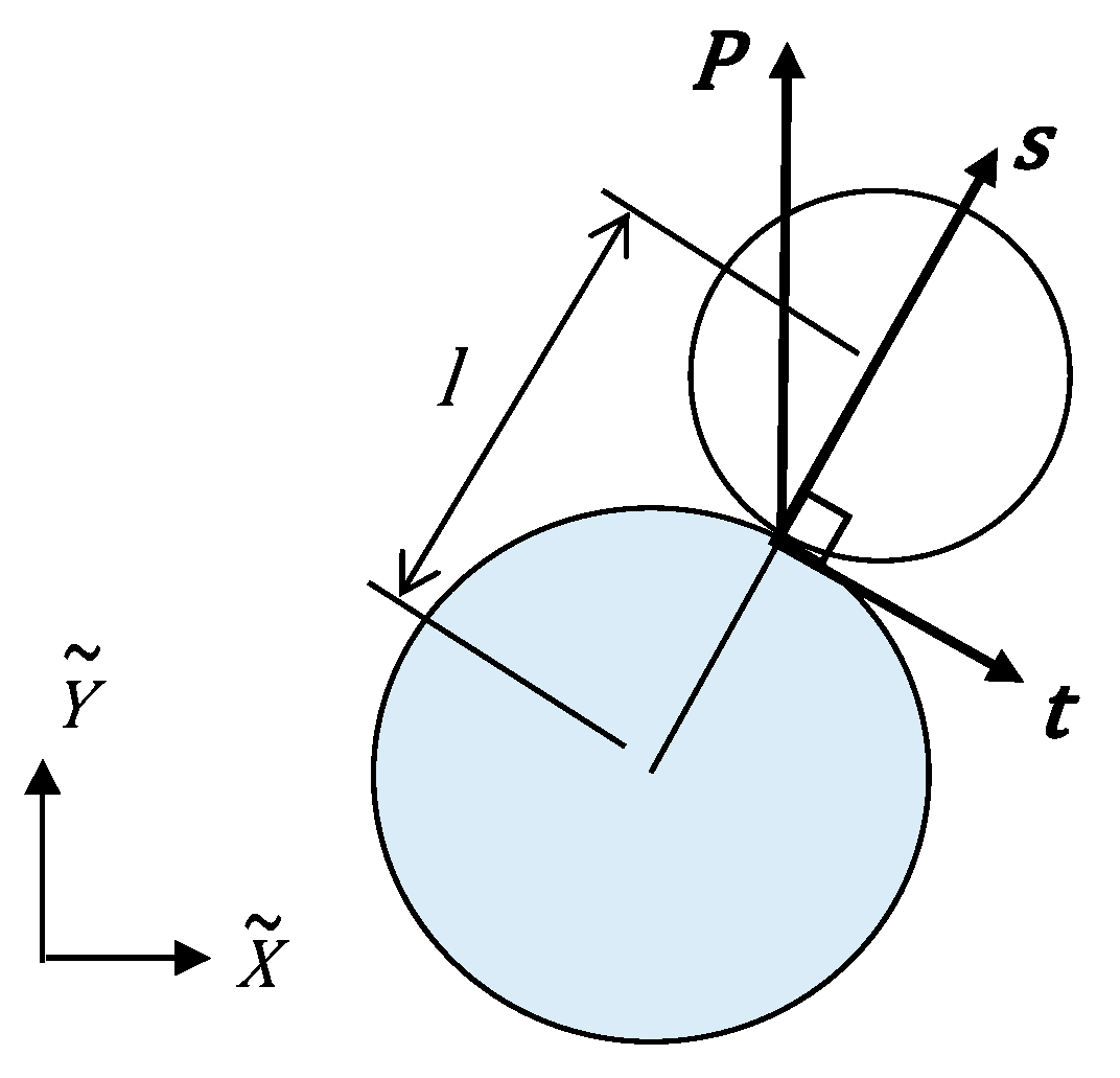
Figure 1 shows the concept of the multiple shear mechanism model, which is based on the granular material. This contact force $\mathit{P}$ shown in this figure is expressed by the following equation in the concept

$$\mathit{P}=f_s\mathit{s}+f_t\mathit{t}.$$

(1)

where $\mathit{s}$ is the normal vector of the contact surface of the granular material, $\mathit{t}$ is the tangential vector, and $f_s$ and $f_t$ are forces acting on the contact surface in the respective directions. The macroscopic stress is determined by the average of the contact forces within a representative volume element with volume $V$, as written in Equation (2), where $l$ represents the distance between the particle centers on each contact surface.

$$\mathit{\sigma }=\frac{1}{V}\sum l\left(f_s\mathit{s}\otimes \mathit{s}+f_t\mathit{s}\otimes \mathit{t}\right).$$

(2)

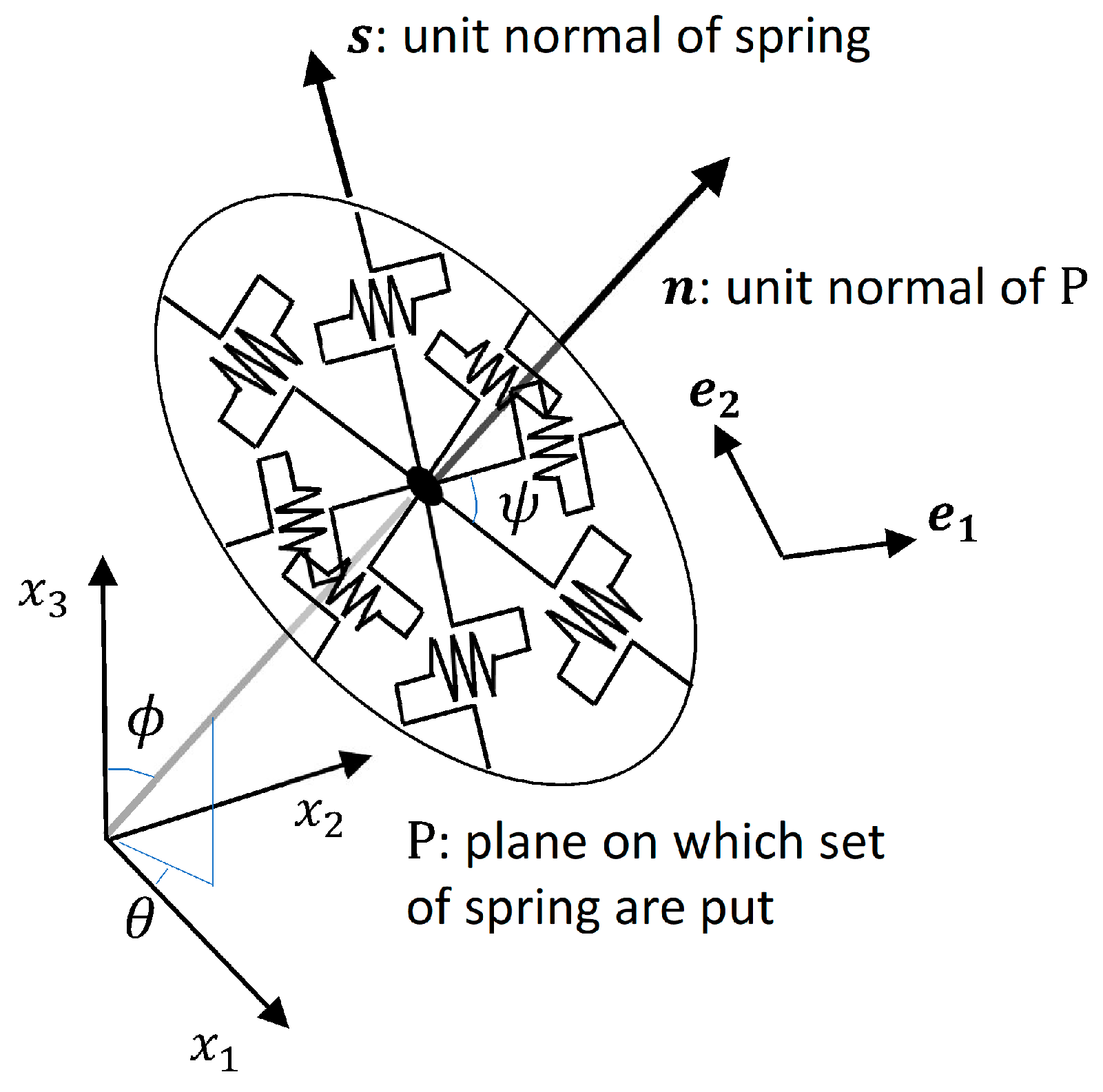
The schematic view of the original model is shown in Figure 2. Given a plane $P$ with a unit normal vector $\mathit{n}$, a circle is placed over it and a spring is placed in the direction of unit normal vector $\mathit{s}$. The shearing direction of this spring on the plane $P$ is $\mathit{t}=\mathit{n}\times \mathit{s}$. Assuming $\tau$ to be the shear stress component generated by the spring, it contributes $\tau \mathit{s}\otimes \mathit{t}$ to the stress tensor. Using unit vectors ${\mathit{e}}_1$ and ${\mathit{e}}_2 \left(={\mathit{e}}_1\times \mathit{n}\right)$, which are orthogonal in plane $P$, $\mathit{s}$ can be expressed as $\mathit{s}=\cos \psi {\mathit{e}}_1+\sin \psi {\mathit{e}}_2$. The contribution of all nonlinear springs in the plane $P$ is

$$\mathit{T}={{\displaystyle \int }}_0^{2\pi }\tau \mathit{s}\otimes \mathit{t} \mathrm{d}\psi .$$

(3)

When the strain tensor is ε, the shear strain component in the $\mathit{s}$ direction on the plane is expressed by the following equation

$$\gamma =\mathit{\epsilon }:\left(\mathit{s}\otimes \mathit{t}\right).$$

(4)

Let $f$ be a hyperbolic function, and then the stress–strain relationship of each spring can be expressed by the equation

$$\tau =f\left(\mathsf{\gamma }\right).$$

(5)

When the unit normal vector of the circle $\mathit{n}$ is a three-dimensional vector and this vector component is expressed as $\left(\sin \varphi \cos \theta ,\sin \varphi \sin \theta ,\cos \varphi \right)$, the springs of all planes generate the following stress tensor $\mathit{\sigma }$.

$$\mathit{\sigma }={{\displaystyle \int }}_0^{2\pi }{{\displaystyle \int }}_0^{\pi }\left({{\displaystyle \int }}_0^{2\pi }\tau \mathit{s}\otimes \mathit{t} \mathrm{d}\psi \right)\sin \varphi \mathrm{d}\varphi \mathrm{d}\theta .$$

(6)

The contribution of isotropic pressure $p$ is excluded from Equation (6). Since $\tau$ is calculated by using the right-hand side of Equations (4) and (5), Equation (6) becomes the symmetric tensor.

By setting Equation (6) to the incremental form, the following equation can be derived

$$\mathrm{d}\mathit{\sigma }=\mathit{D}:\left(\mathrm{d}\mathit{\epsilon }-\mathrm{d}{\mathit{\epsilon }}_{\mathit{d}}\right)$$

(7)

where ${\mathit{\epsilon }}_{\mathit{d}}$ is the strain tensor of the isotropic component and $\mathit{D}$ is the fourth-order tensor of

$$\mathit{D}={{\displaystyle \int }}_0^{2\pi }{{\displaystyle \int }}_0^{2\pi }{{\displaystyle \int }}_0^{\pi }{f}^{\prime }\left(\gamma \right)\left(\mathit{s}\otimes \mathit{t}+\mathit{t}\otimes \mathit{s}\right)\otimes \frac{1}{2}\left(\mathit{s}\otimes \mathit{t}+\mathit{t}\otimes \mathit{s}\right)\sin \varphi \mathrm{d}\varphi \mathrm{d}\theta \mathrm{d}\psi$$

(8)

where $f^{\prime }$ is the derivative of the hyperbolic function $f$ and $\mathit{D}$ corresponds to a nonlinear constitutive relation tensor.

The right-hand sides of Equations (6) and (8) use a triple integral using three variables $\left(\theta ,\varphi ,\mathrm{and}\psi \right)$. In particular, in order to calculate Equation (8), the parameters of hyperbolic function $f$ [7] must be set corresponding to the three variables. To execute this triple integration accurately, an enormous amount of memory is required. In order to implement the original model for FEM, it is necessary to store the parameters related to the hyperbolic function of all the springs in order to create the overall stiffness matrix, which requires enormous amounts of memory.

2.2. Concept of the Proposed Model

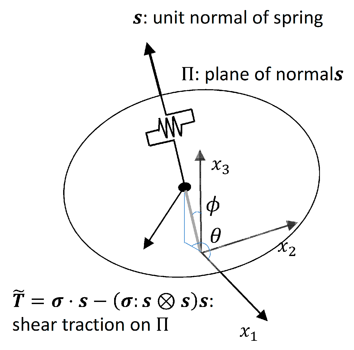
As shown in [13], we develop an alternative formulation (the proposed model) suitable for large-scale three-dimensional FEM based on the multiple shear mechanism model. The concept of the proposed model is shown in Figure 3. In the proposed model, every spring is handled as being connected to the origin in three-dimensional space, and $\mathit{s}$ in Figure 3 is a unit normal vector whose direction is orthogonal to plane $\mathsf{\Pi }$ (as a plane that is orthogonal to the spring direction $\mathit{s}$ and is used to compute shear traction). If the stress tensor at the origin is $\mathit{\sigma }$, the traction acting on $\mathsf{\Pi }$ can be expressed as $\mathit{\sigma }·\mathit{s}$. Since the axis component of this traction is $\mathit{\sigma }:\mathit{s}\otimes \mathit{s}$, which is a scalar value, the shear traction on $\mathsf{\Pi }$ is the following vector.

$$\tilde{\mathit{T}}=\mathit{\sigma }\cdot \mathit{s}-\left(\mathit{\sigma }:\mathit{s}\otimes \mathit{s}\right)\mathit{s}.$$

(9)

Let the normal vector to the direction of $\tilde{\mathit{T}}$ be expressed by ${\mathit{s}}^{\prime }$ and then we can represent the shear component of $\tilde{\mathit{T}}$ as $\tilde{\tau }=\tilde{\mathit{T}}·{\mathit{s}}^{\prime }$.

It is possible to calculate scalar $\tilde{\gamma }$, which is the shear strain component in the direction of ${\mathit{s}}^{\prime }$ the plane $\mathsf{\Pi }$ from strain tensor $\mathit{\epsilon }$. We assumed that $\tilde{\tau }$ and $\tilde{\gamma }$ satisfy the following equation with the hyperbolic function $f$

$$\tilde{\tau }=f\left(\tilde{\gamma }\right).$$

(10)

Therefore, when $\mathit{s}$ is expressed as $\left(\sin \varphi \cos \theta ,\sin \varphi \sin \theta ,\cos \varphi \right)$, the stress tensor can be expressed by the following integration for all springs

$$\mathit{\sigma }={{\displaystyle \int }}_0^{2\pi }{{\displaystyle \int }}_0^{\pi }\tilde{\tau }\left(\mathit{s}\otimes {\mathit{s}}^{\prime }+{\mathit{s}}^{\prime }\otimes \mathit{s}\right)\sin \varphi \mathrm{d}\varphi \mathrm{d}\theta$$

(11)

where the contribution of isotropic pressure $p$ is excluded.

The stress tensor in the incremental formulation can also be expressed by the equation

$$\mathrm{d}\mathit{\sigma }=\tilde{\mathit{D}}:\left(\mathrm{d}\mathit{\epsilon }-\mathrm{d}{\mathit{\epsilon }}_{\mathit{d}}\right)$$

(12)

where

$$\tilde{\mathit{D}}=\iint f^{\prime }\left(\tilde{\gamma }\right)\left(\mathit{s}\otimes {\mathit{s}}^{\prime }+{\mathit{s}}^{\prime }\otimes \mathit{s}\right)\otimes \frac{1}{2}\left(\mathit{s}\otimes {\mathit{s}}^{\prime }+{\mathit{s}}^{\prime }\otimes \mathit{s}\right)\sin \varphi \mathrm{d}\varphi \mathrm{d}\theta .$$

(13)

Similar to $\mathit{D}$ in Equation (8), $\tilde{\mathit{D}}$ in Equation (13) corresponds to a nonlinear constitutive relation tensor. The fourth-order tensor represented by Equation (13) (the proposed model) and Equation (8) (the original model) is different in that Equation (13) is a double integral and Equation (8) is a triple integral.

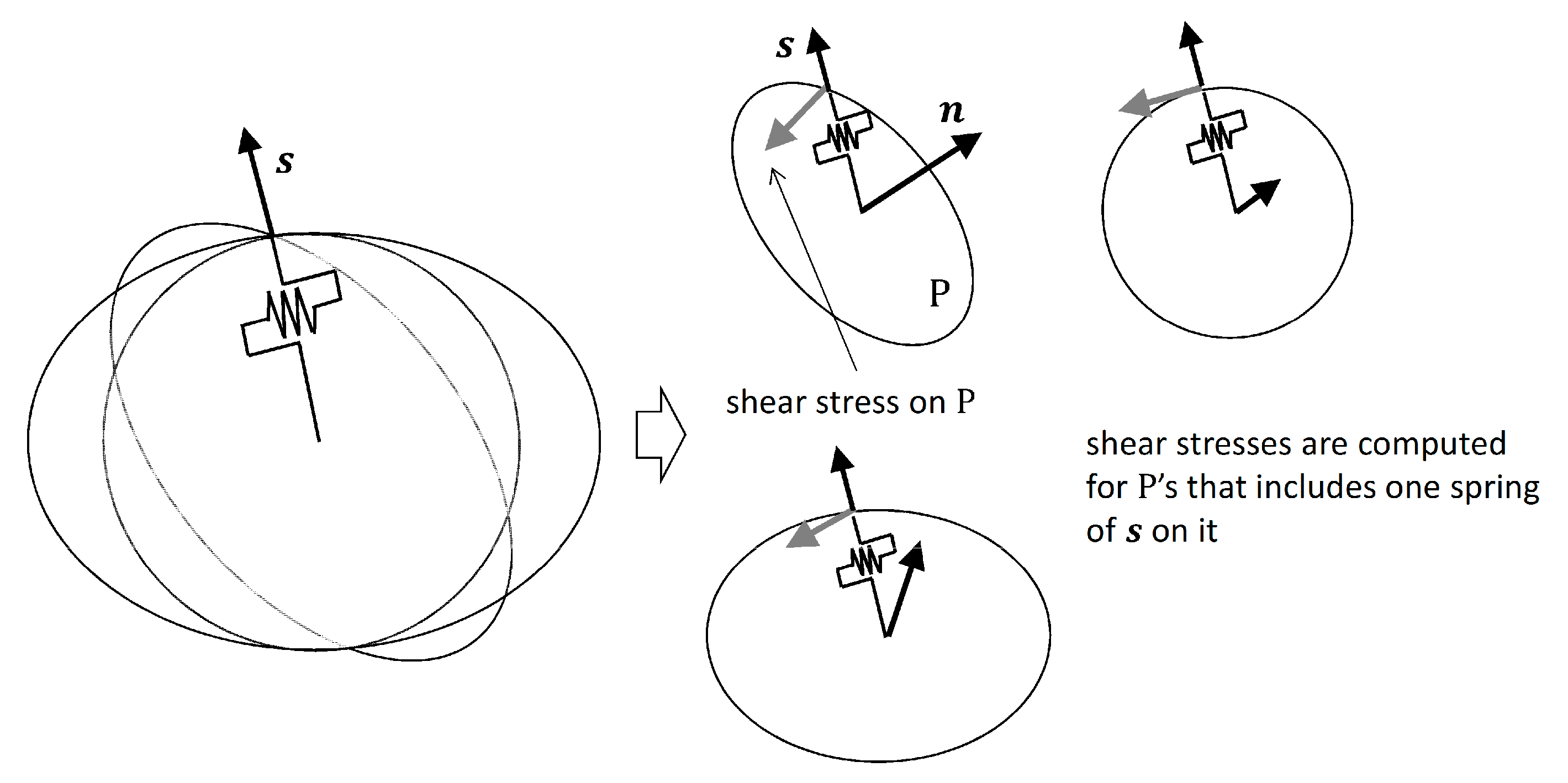
Figure 4 shows a schematic view of the spring treatment used in the original model. In the original model, plane $P$ is first set in three-dimensional space. Next, a plurality of springs is set on plane $P$. Since the plane P is firstly determined in the original model, the spring in the $\mathit{s}$ direction is used in all planes P, which have $\mathit{s}$. In the proposed model, a spring in an arbitrary direction is first set in three-dimensional space, and a plane $\mathsf{\Pi }$ perpendicular to the direction is defined. Therefore, in the proposed model, a spring in any direction is used only once. As a result, the triple integral of Equation (8) can be contracted to the double integral of Equation (13).

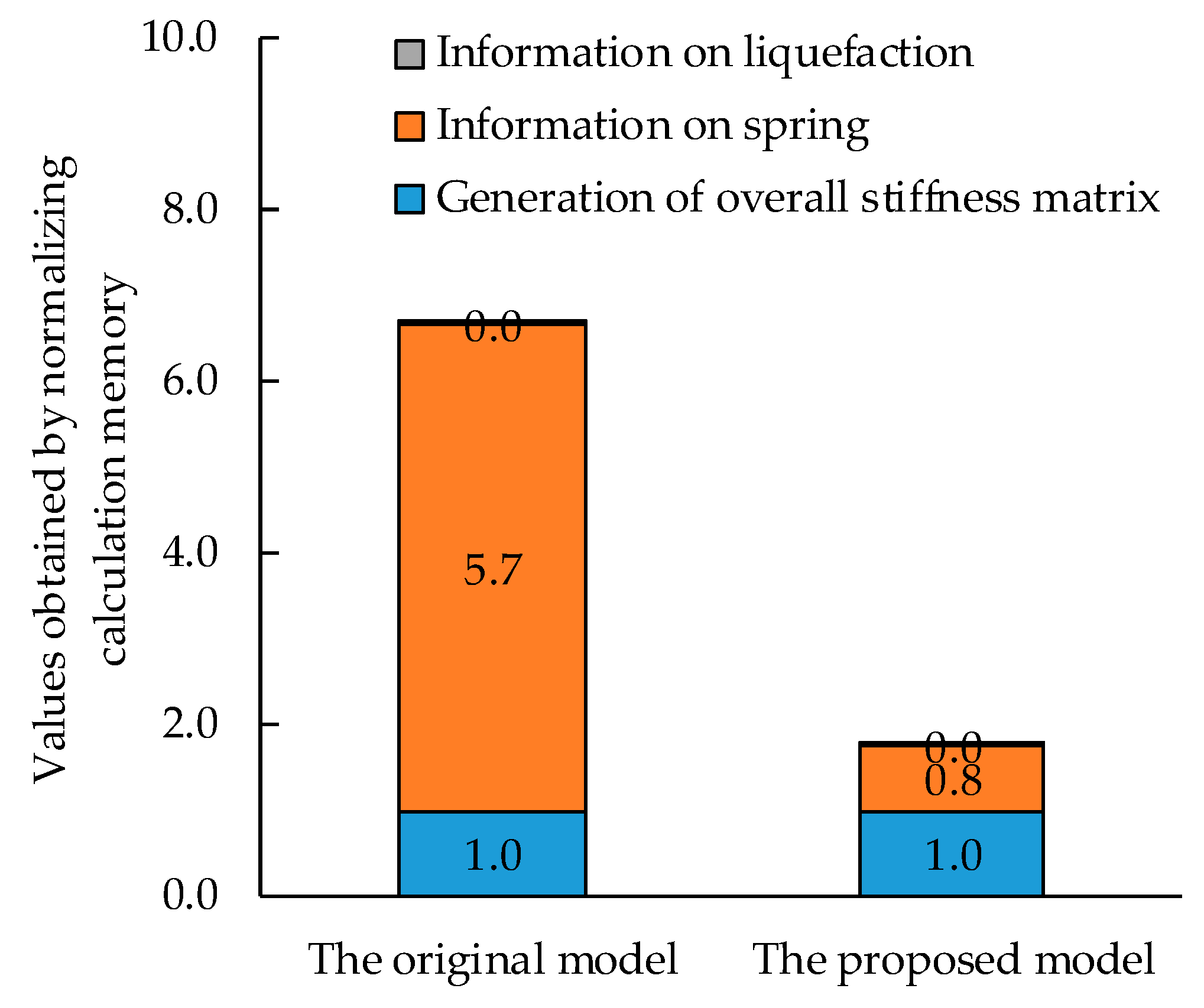
From a numerical analysis viewpoint, it is important to contract triple integration to double integration to reduce the amount of memory. In the case where there are $M$ triple integral variables $\left(\theta ,\varphi ,\psi \right)$ and double integral variables $\left(\theta ,\varphi \right),$ $M^3$ springs in Equation (8) and $M^2$ springs in Equation (13) are considered. Also, the required memory for storing the hyperbolic function parameters of each spring increases with the number of springs.

There are multiple springs in the $\mathit{s}$ direction in the original model and the resultant force of the shear stress components of these springs is theoretically equivalent to those of the proposed model in the ${\mathit{s}}^{\prime }$ direction. The direction of the shear stress component vector $\tilde{\mathit{T}}$, which is generated in the direction of ${\mathit{s}}^{\prime }$, sequentially changes on plane $\mathsf{\Pi }$. That is, the direction ${\mathit{s}}^{\prime }$ of $\tilde{\mathit{T}}$ varies with every time step. Therefore, ${\mathit{s}}^{\prime }$ calculated from $\tilde{\mathit{T}}$ is used in Equation (13) and $\tilde{\gamma }$ is the shear strain component calculated by the following equation using time-invariant $\mathit{s}$ and time-variant ${\mathit{s}}^{\prime }$

$$\tilde{\gamma }=\mathit{\epsilon }:\frac{1}{2}\left(\mathit{s}\otimes {\mathit{s}}^{\prime }+{\mathit{s}}^{\prime }\otimes \mathit{s}\right).$$

(14)

The major differences between the original model and the proposed model are as follows. In the original model, the total stiffness matrix is calculated based on the shear strain generated in each spring having a predetermined direction. In the proposed model, the total stiffness matrix is calculated based on the maximum shear strain component generated on a certain plane. Therefore, in situations where the stress field suddenly changes from place to place, the original model may miss the maximum shear strain component occurring on the planes, and so there is a possibility of overestimating the overall stiffness matrix.

2.3. Verification of the Proposed Model

To use the proposed model for practical design work, it is important to show that the proposed model is capable of simulating the response as well as the original model. Furthermore, it is necessary to show that the accuracy can be secured without significantly increasing the total number of springs when the mechanical characteristics of adjacent springs do not change abruptly in the proposed model. In this section, we verify the validity of the proposed model by comparing the responses simulated by the proposed model with the original model by the case of using a single solid element.

First, we performed a numerical simulation against cyclic simple shear loading using the finite element total stress analysis method with a single solid element. The input property values used in this study were determined using the method proposed by Morita et al. [14] for sand whose equivalent SPT N value is 10. The loading condition was simple shearing with the maximum shear stress being 30 kPa. The number of planes P and springs on plane P of the original model were changed in this numerical simulation in order to confirm the influence on the response value. Similarly, the number of springs in the proposed model was also changed. For the integration of Equations (8) and (13), the discrete-ordinate method (Sn method) [15], which is known as a method for integrating solid angle with high accuracy, was used. Each spring was installed symmetrically in three-dimensional space in order to reduce the amount of memory for both the original and the proposed model.

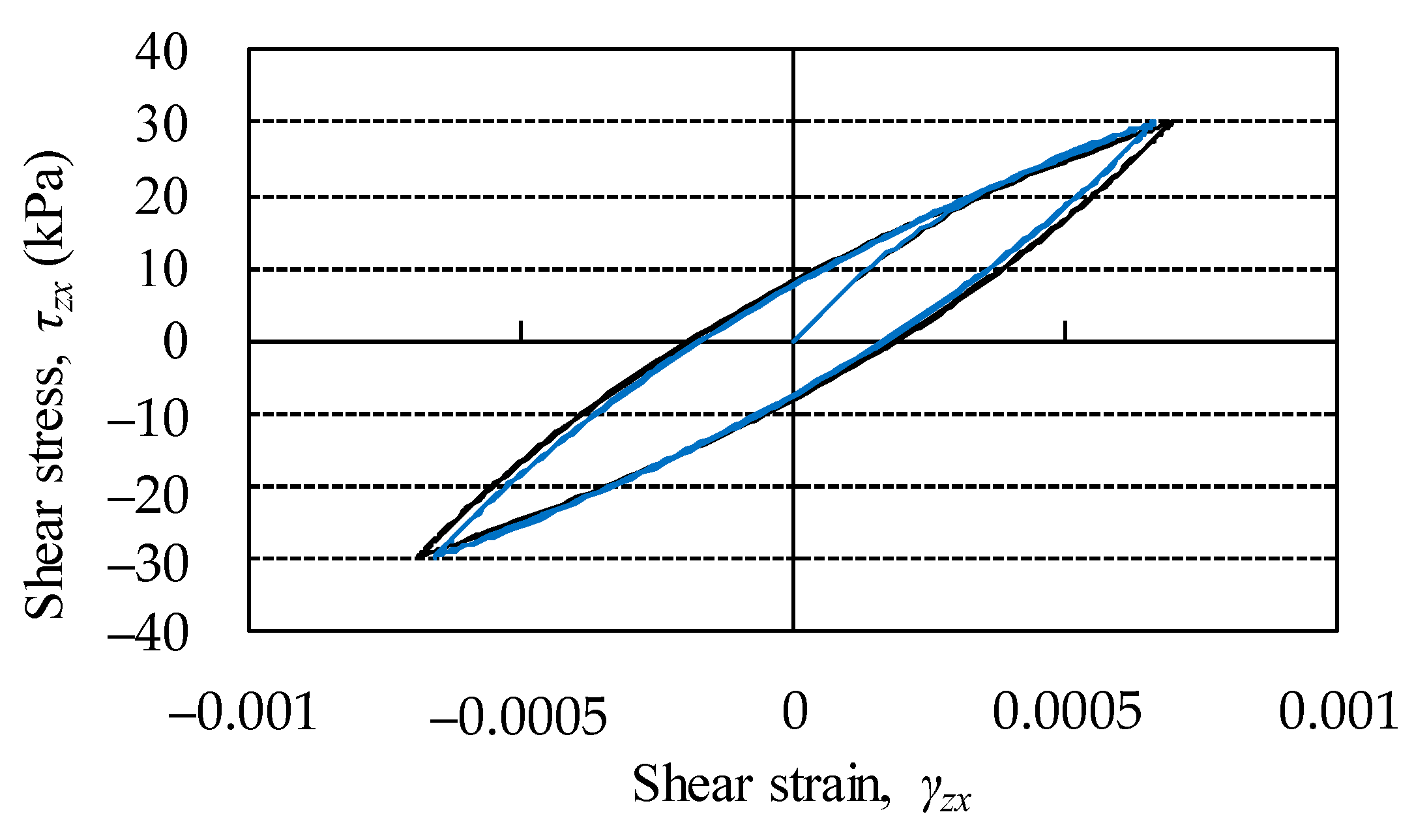
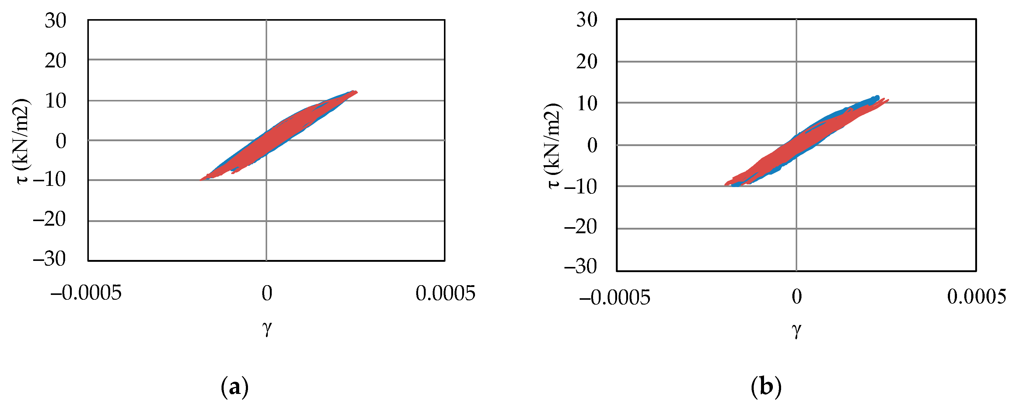
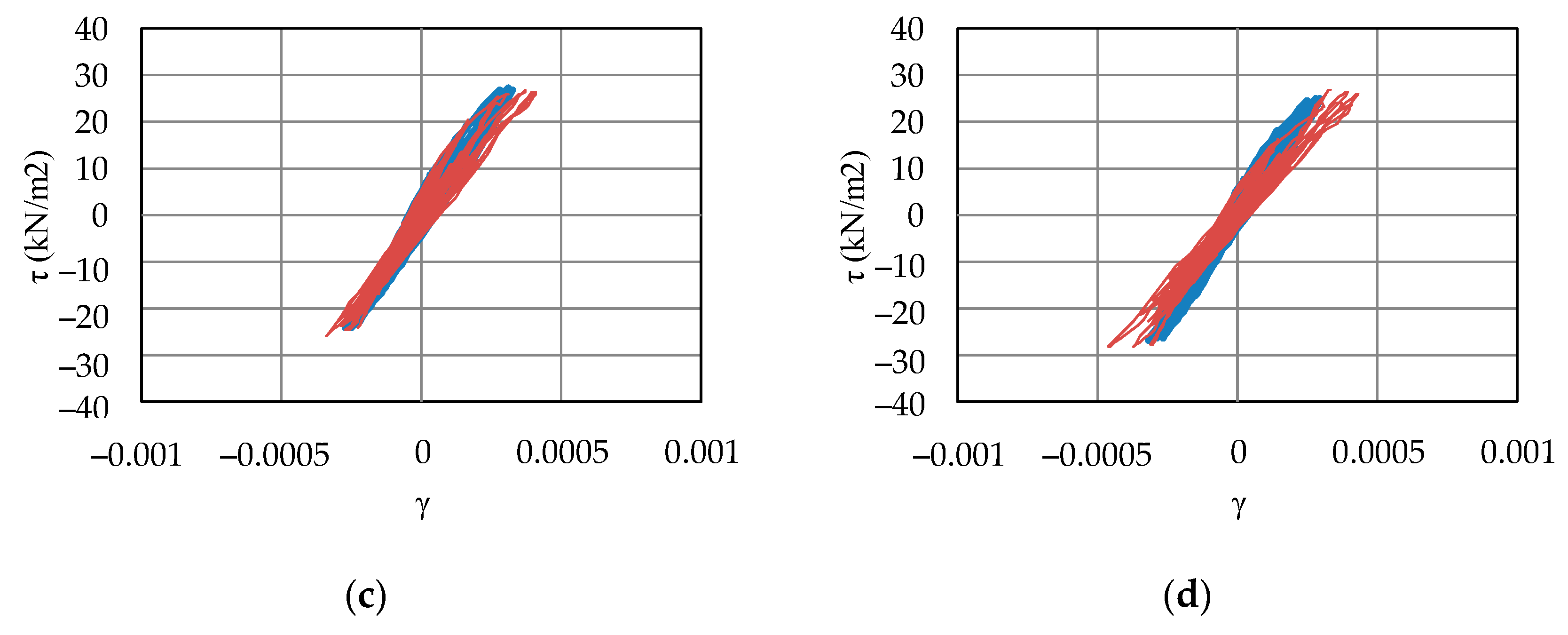
The comparison between the shear stress–shear strain relation of the original model and the proposed model is shown in Figure 5. In this simulation, the number of planes $P$ in the original model was 144 per hemisphere and the number of springs on the plane $P$ was 12 per semicircle (total number of springs was 1728). The number of springs of the proposed model was set to 144 per hemisphere. In the proposed model, despite using only 1/12th of the springs of the original model, a highly consistent result with less than 5% relative error compared to the original model was obtained.

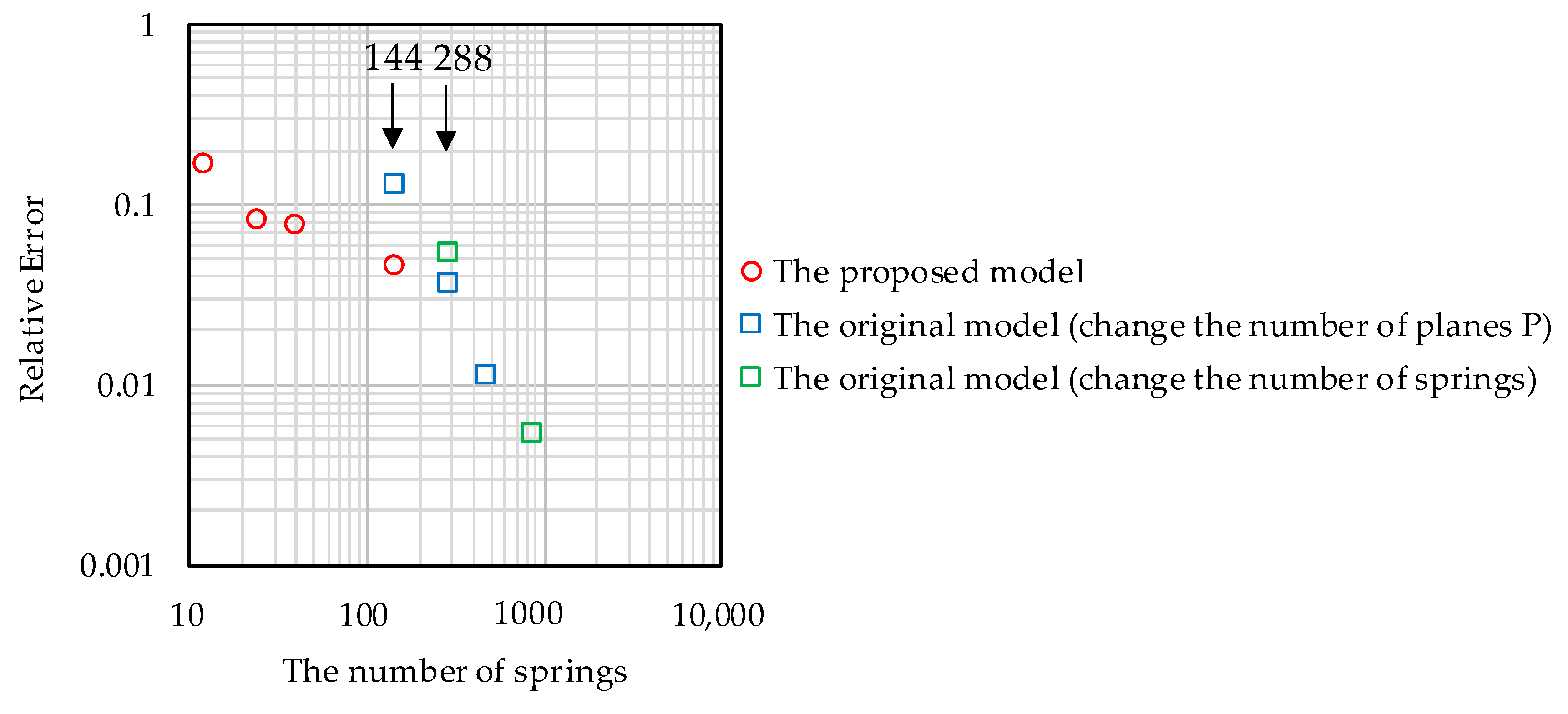
Figure 6 shows the relative error when changing the number of springs. For the original model, the number of planes $P$ and the number of springs on plane $P$ were changed separately. The relative error is calculated by the equation

$$Relative Error=\frac{|{\gamma }_{zx}-{\gamma }_{zx,\mathrm{real}}|}{{\gamma }_{zx,\mathrm{real}}}.$$

(15)

When calculating this relative error, the value of ${\gamma }_{zx}$, when the load ${\tau }_{zx}$ was 30 kPa, was used in every case. Here, ${\gamma }_{zx,\mathrm{real}}$ is set as the value obtained in the case where the number of planes $P$ is 144 per hemisphere and the number of springs on the plane $P$ is 12 per semicircle in the original model.

As shown in Figure 6, the relative error decreased as the number of springs increased in both models. When the total number of springs was the same in both models, the relative error was smaller in the proposed model than in the original model, as indicated in the previous section. Focusing on the plots given the same degree of relative error in Figure 6, we found that the number of springs of the original model was 288 and the number of springs of the proposed model was 144. That is, in this example, the simulation cost of the proposed model with the same relative error is only about one-half that of the original model. This indicates that the proposed model has an extremely high ability to execute soil non-linear analysis targeting large-scale three-dimensional problems.

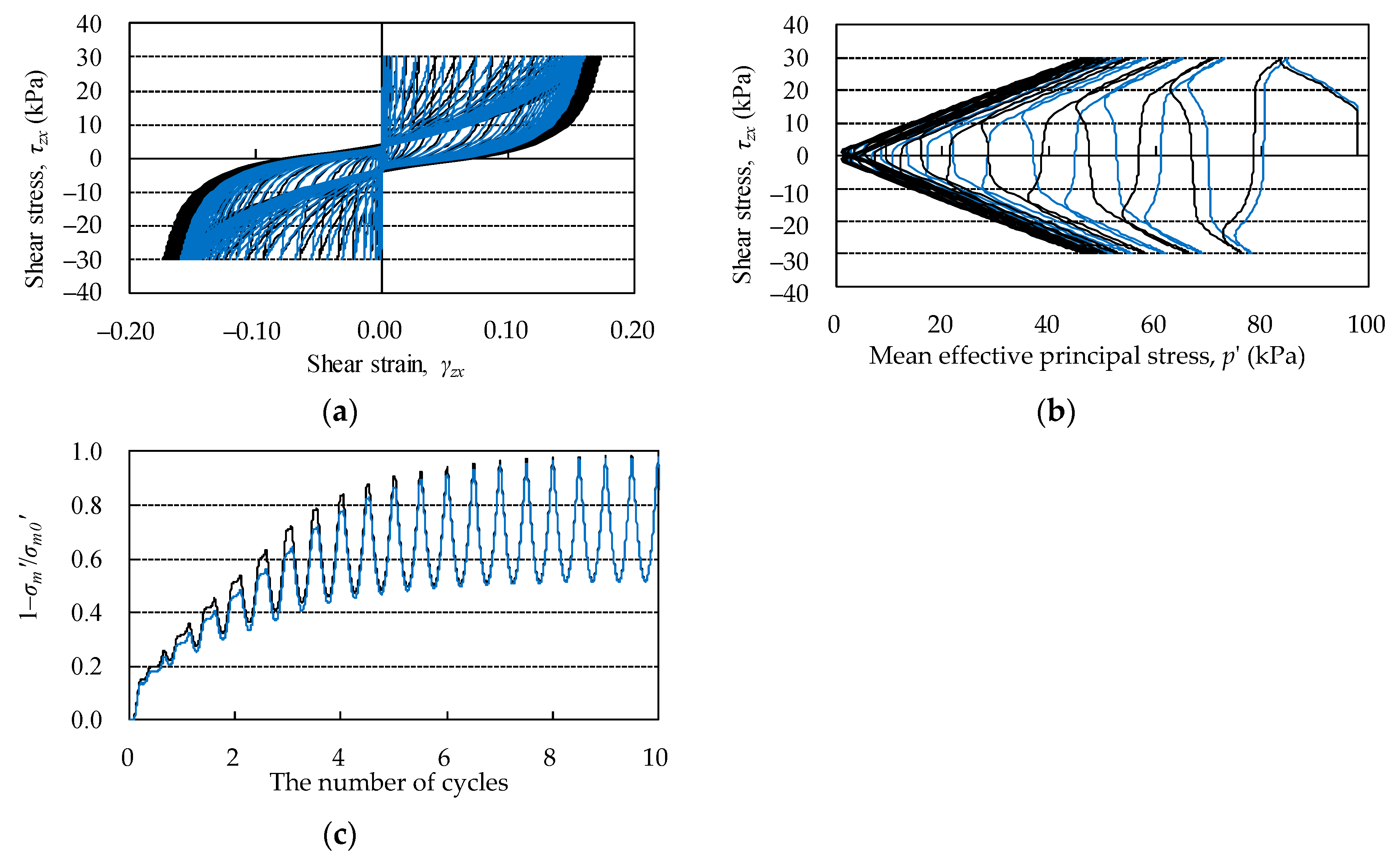
Next, we analyzed the effective stress of both the original and the proposed models to determine the effect of increasing the excess pore water pressure. The input property values and boundary conditions were the same as during the cyclic simple shear test (total stress analysis). The number of planes $P$ of the original model was 144 per hemisphere and the number of springs on the plane $P$ was 12 per semicircle. As for the proposed model, the number of total springs was set to 144 per hemisphere.

A comparison of responses obtained by both models is shown in Figure 7. We found that there was little difference among the shear stress–shear strain relation, mean effective principal stress path, and excess pore water pressure ratio obtained by both models. The reason for this finding is due to the fact that the original model tends to overestimate the overall stiffness matrix. Although slight differences in responses were found between both models, it does not cause any problems from the viewpoint of practical designing work.

3. Analyses Using a High-Fidelity Analysis Model of Soil and a Structure

3.1. Problem Settings

In this section, effective stress analyses with both the original and the proposed models are carried out against three-dimensional high-fidelity model with over 1 million degrees of freedom (DoF). The model is shown in Figure 8, which is the standard model of U.S. Department of Energy (DOE) for evaluating the effect of the dynamic interaction responses between reactor building and soil under earthquakes.

Figure 9 shows the building part in the model. Solid elements are used for the part of concrete and shell elements are used for the part of reinforcement. The specification of the characteristic values for the parts of the building are shown in

Table 1. Deformation characteristic parameters of the reactor building used for the simulation

Type	Young Modulus	Poisson’s Ratio	Density
	E (kPa)	Ν	$\mathit{\rho }$
Concrete	45,490,000	0.30	2.4
Reinforcement	205,000,000	-	-

.

The soil and rock parts of the model are shown in Figure 10. In the original DOE model, all base ground parts are defined as a linear elastic body, but we changed this part to a nonlinear elastic body in order to evaluate the performance of both the original and the proposed models studied in Section 2 in this paper. The input characteristic values of the soil and rock for this simulation were set referring to the values that were used during the safety review for restarting the Kashiwazaki-Kariwa Nuclear Power Station [16]. The specification of the characteristic values for the parts of this model are shown in

Table 2. Deformation characteristics parameters of the soil and rock used for the simulation. The parameter designations are illustrated in [9].

Type	Shear Modulus	Bulk Modulus	Reference Confining Pressure	Poisson’s Ratio	Reduction Factor of Shear and Bulk Modulus	Internal Friction Angle	Cohesion	Upper Bound for Hysteretic Damping Factor
	Gma (kPa)	Kma (kPa)	σma’ (kPa)	Ν	m	Φf (degree)	c (kPa)	hmax
Layer of Sand	207,000	540,000	190.0	0.33	0.5	45.0	0.0	0.155
Nishiyama Layer	415,000	1,080,000	98.0	0.33	0.0	-	-	0.257

and

Table 3. Liquefaction characteristics parameters of the soil used for the simulation. Parameter designations are illustrated in [9].

Type	Phase Transformation Angle	Overall Dilatancy	Initial Phase of Dilatancy	Final Phase of Dilatancy	Threshold limit of Dilatancy	Ultimate limit of Dilatancy
	Φp (degree)	w1	p1	p2	c1	S1
Layer of Sand	28.0	2.40	0.50	0.80	1.92	0.005

. In the original model, the number of planes $P$ was set to 40 per hemisphere using the Sn method and the number of springs on a plane $P$ was 12 per semicircle. As for the proposed model, the number of springs was 40 per hemisphere using the Sn method.

For the boundary condition, a viscous boundary condition was set on the bottom of the rock and the side boundary was free. While there are various numerical analysis methods to handle the lateral virtual boundaries, the best method is not found yet. In this study, to avoid discussion on which method is the best for the lateral virtual boundary condition, used was the model which is sufficiently wide so that the effects of the lateral boundaries on the solution becomes negligible. The white noise shown in Figure 11 was used as the input ground motion. This wave was used as dynamic forces acting simultaneously in three directions as an incident wave after the self-weight analysis of the whole model. Here, the vertical direction of the ground motion was set to half the input wave. The numerical conditions are shown in

Table 4. Numerical conditions for the high fidelity analysis model used for the simulation

Category	Item	Numerical Conditions
Non-linear calculation	Iterative method	Newton-Raphson method
	Convergence criterion	1.0 × 10−8
	Maximum number of iterations	100
	Dynamic step	0.01 s/step
	Total step	1536 (15.36 s)
Method to solve the inverse matrix	Solver	CG method
	Precondition	Slice Successive Over Relaxation
	Convergence criterion	1.0 × 10−8
	Maximum number of iterations	100,000
	The number of parallel	2~128

. The numerical integration method uses the Newmark-β method ($\beta =0.25,\gamma =0.5$). Based on the result of the eigenvalue analysis for the whole model, the coefficients $\alpha$ and $\beta$ of the mass matrix and stiffness matrix for Rayleigh damping factor formulation were set to $\alpha =0.844\mathrm{and}\beta =0.00296$. The CPU of the computer used for this simulation was an Intel Xeon E5-2697v2 (2.7 GHz) (Intel Corp., Tokyo, Japan).

3.2. Comparison of the Original Model with the Proposed Model

The shear stress–shear strain relation of the soil is shown in Figure 12 and we found that the results of both models were very similar to each other. As described in Section 2, the stiffness of the soil of the original model was overestimated, so the maximum shear strain of the original model was slightly lower than in the proposed model. The shear strain distribution of the soil at the final time step is shown in Figure 13. As can be seen from the figure, both results showed good consistency.

The excess pore water pressure ratio distribution at the final time step is shown in Figure 14. The proposed model produced slightly higher excess pore pressure than the original model, but the distributions of both models were relatively very similar. For both models, the maximum value of the excess pore water pressure ratio exceeded 0.5.

Figure 15 shows the memory used for the both models in this simulation. The values of the memory were normalized by the reference memory that is used to store the overall stiffness matrix. As mentioned in Section 2, this result showed that the memory used for the springs consumed the majority of the required memory in this simulation and the memory for this part was drastically reduced in the proposed model compared with the original model. In the required memory for the finite element analysis as a whole, the proposed model achieved a 74% reduction in the computational memory against the original model.

3.3. Scalability of Computing Liquefaction Processes of Soil

In this section, the scalability of the FEM code, which is implemented both the original model and the proposed model used in this simulation, is explained. Figure 16 shows the execution time when the number of parallel cores is changed on both models. Generally, in the case where the ideal parallel performance is obtained, the execution time is multiplied by the reciprocal of the number of parallel cores. From this figure, we found that the scalability of the simulation can be sufficiently confirmed. In the case of 128 parallel, the time of the proposed model is 5.7 h, which is about half of the execution time of the original model.

Since the calculation of each node exceeds the required memory of the computer being used, it was impossible to analyze the original model in less than 16 cores. This shows that it is practically impossible to calculate models with a very large degrees of freedom using the original model in an ordinary computer environment. Regarding the proposed model, it is capable of simulating the condition with two cores, which indicates that the original model helps in the practical engineering design of important infrastructure with very large numerical models.

4. Closing Remarks

In this study, in order to confirm the robustness of the developed parallel FEM considering the effectiveness of liquefaction evaluation, three studies were conducted. First, we proposed the multiple shear mechanism model with drastically reduced the memory, called ‘the proposed model’, in order to apply the concept of the multiple shear mechanism model to large scale three-dimensional FEM. Next, we conducted some comparative numerical studies with the proposed model and the original model. We confirmed that the results of simulations from both models were highly consistent with each other. The proposed model drastically reduced the required memory and the execution time compared with the original model. Lastly, the scalability of the soil liquefaction process using the developed parallel FEM was investigated. We demonstrated that the developed parallel FEM has high scalability and we confirmed that the execution time required for a given analysis could be well estimated in advance of the simulation. This result is advantageous from the viewpoint of using a high-fidelity model necessary for liquefaction analysis.

Through this study, we confirmed that very large-scale earthquake response analysis considering liquefaction could be conducted in less than half a day with the developed FEM built in the proposed model. We also highlighted the limitation of degrees of freedom in the problem, which can be analyzed in the current computing environment for practical design work.

We think that the results shown in this paper provide useful information for developing and maintaining future parallel computational environments.

References

1. Yamashita, T.; Miyamura, T.; Akiba, H.; Kajiwara, K. Verification of finite element Elastic-plastic buckling analysis of square steel tube column using solid elements. Trans. Jpn. Soc. Comput. Eng. Sci. 2013, 1, 20130001. (In Japanese) [Google Scholar]
2. Miyamura, T.; Yamashita, T.; Akiba, H.; Ohsaki, M. Dynamic FE simulation of four-story steel frame modelled by solid elements and its validation using results of full-scale shake-table test. Earthq. Eng. Struct. Dyn. 2014, 44, 1449–1469. [Google Scholar] [CrossRef]
3. FrontISTR Forum. FrontISTR ver.4.5. Available online: http://www.multi.k.u-tokyo.ac.jp/FrontISTR/files/FISTRv4.5E.pdf (accessed on 14 September 2018). (In Japanese).
4. Iai, S.; Matsunaga, Y.; Kameoka, T. Strain space plasticity model for cyclic mobility. Soils Found. 1990, 29, 27–56. [Google Scholar] [CrossRef]
5. Towhata, I.; Ishihara, K. Modelling soil behavior under principal stress axes rotation. In Proceedings of the 5th International Conference on Numerical Methods in Geomechanics, Nagoya, Japan, 5 April 1985; pp. 523–530. [Google Scholar]
6. Iai, S. Micromechanical background to a strain space multiple mechanism model for sand. Soils Found. 1993, 33, 102–117. [Google Scholar] [CrossRef]
7. Iai, S.; Matsunaga, Y.; Kameoka, T. Parameter Identification for a Cyclic Mobility Model; Report of the Port and Harbour Research Institute; Port and Harbour Research Institute: Yokosuka, Japan, 1990; Volume 29, pp. 57–83. [Google Scholar]
8. Iai, S. Three dimensional formulation and objectivity of a strain space multiple mechanism model for sand. Soils Found. 1993, 33, 192–199. [Google Scholar] [CrossRef]
9. Iai, S.; Ozutsumi, O. Yield and cyclic behaviour of a strain space multiple mechanism model for granular materials. Int. J. Numer. Anal. Meth. Geomech. 2005, 29, 211–240. [Google Scholar] [CrossRef]
10. Iai, S.; Kameoka, T. Finite element analysis of earthquake induced damage to anchored sheet pile quay walls. Soils Found. 1993, 33, 71–91. [Google Scholar] [CrossRef]
11. Iai, S.; Morita, T.; Kameoka, T.; Matsunaga, Y.; Abiko, K. Response of a dense sand deposit during 1993 Kushiro-Oki earthquake. Soils Found. 1995, 35, 115–131. [Google Scholar] [CrossRef]
12. Ozutsumi, O.; Sawada, S.; Iai, S.; Takeshima, Y.; Sugiyama, W.; Shimazu, T. Effective stress analyses of liquefaction-induced deformation in river dikes. Soil Dyn. Earthq. Eng. 2002, 22, 1075–1082. [Google Scholar] [CrossRef]
13. Hotta, W.; Suzuki, S.; Hori, M. Contraction of multiple shear mechanism model for large scale three-dimensional finite element method analyses and verification between original and the contracted model. J. Jpn. Soc. Civ. Eng. Ser. A2. submitted on 7th September 2018. (In Japanese).
14. Morita, T.; Iai, S.; Liu, H.; Ichii, K.; Sato, Y. Simplified Method to Determine Parameter of FLIP; Technical Note of the Port and Harbour Research Institute, No. 869; Port and Harbour Research Institute: Yokosuka, Japan, 1997. (In Japanese) [Google Scholar]
15. Ikeda, H.; Takeda, T. A new nodal SN transport method for three-dimensional hexagonal geometry. J. Nucl. Sci. Technol. 1994, 31, 497–509. [Google Scholar] [CrossRef]
16. Tokyo Electric Power Company Holdings. Available online: http://www.tepco.co.jp/about/power_station/disaster_prevention/2017/pdf/nuclear_power_170124_04.pdf (accessed on 19 October 2018). (In Japanese).
Figure 1. Concept of multiple shear mechanism: normal vector s , tangential vector t , and contact force P .
Geosciences 09 00038 g001
Figure 2. Schematic view of the original mode.
Geosciences 09 00038 g002
Figure 3. Schematic view of the proposed model.
Geosciences 09 00038 g003
Figure 4. Schematic view of spring treatment used in original model; the spring in the s direction is to be used in all planes P that have springs in direction s .
Geosciences 09 00038 g004
Figure 5. The comparison between the shear stress–shear strain relation of the original model with the proposed model. Black line is shown as the response of the original model and blue line is shown as that of the proposed model.
Geosciences 09 00038 g005
Figure 6. The relative error due to difference in the number of springs against cyclic simple shear loading by finite element total stress analysis method with a single solid element; when the load τ z x of 30 kPa was used.
Geosciences 09 00038 g006
Figure 7. Comparisons of responses against the cyclic simple shear test by both the original and the proposed models with increasing the excess pore water pressure: (a) shear stress–shear strain relation, (b) mean effective principal stress path, and (c) time history of excess pore water pressure ratio. Black lines represent the responses of the original model and blue lines represent those of the proposed model.
Geosciences 09 00038 g007
Figure 8. The high-fidelity analysis model for evaluating the effect of dynamic interactions between a reactor building and soil under an earthquake.
Geosciences 09 00038 g008
Figure 9. Details of the part of the reactor building in the high-fidelity analysis model; solid elements are used for the part of concrete and shell elements are used for the part of reinforcement.
Geosciences 09 00038 g009
Figure 10. Schematic view of the part of the soil, rock and man-made rock; the points to be evaluated are shown in red-circles.
Geosciences 09 00038 g010
Figure 11. The input ground motion (white noise); this wave was input simultaneously in three directions as an incident wave.
Geosciences 09 00038 g011
Figure 12. Shear stress–shear strain relations: (a) the response in YZ direction in upper layer of sand, (b) the response in ZX direction in upper layer of sand, (c) the response in YZ direction in lower layer of sand, and (d) the response in ZX direction in lower layer of sand. Blue line is the response of the original model and red line is that of the proposed model.
Geosciences 09 00038 g012aGeosciences 09 00038 g012b
Figure 13. Shear strain distribution of ZX direction (15.36 s) in (a) the original model and (b) the proposed model.
Geosciences 09 00038 g013
Figure 14. The excess pore water pressure ratio distribution at 15.36 s in (a) the original model and (b) the proposed model.
Geosciences 09 00038 g014aGeosciences 09 00038 g014b
Figure 15. Required memory of finite element analysis in the high fidelity model using multiple shear mechanism model and excess water pore pressure model.
Geosciences 09 00038 g015
Figure 16. Execution time of the simulation with various numbers of cores. Blue points denote the time of the original model and red points denote the time of the proposed model.
Geosciences 09 00038 g016