Article

Six Years Temperature Monitoring Using Fibre-Optic Sensors in a Bioreactor Landfill

1
Irstea, UR PROSE, CS 10030, F-92761 Antony CEDEX, France
2
SAS Les Champs Jouault, Lieu-dit Les Champs Jouault, 50670 Cuves, France
3
Irstea, UR REVERSAAL, F-69626 Villeurbanne CEDEX, France
*
Author to whom correspondence should be addressed.
Submission received: 9 September 2019 / Revised: 27 September 2019 / Accepted: 30 September 2019 / Published: 2 October 2019
(This article belongs to the Special Issue Subsurface Thermography and the Use of Temperature in Geosciences)

Abstract

:
Temperature is a relevant physical parameter to monitor the biodegradation phases of waste mass. Irstea and the landfill operator SAS Les Champs Jouault have been collaborating since 2011 to study the temporal evolution and the spatial distribution of temperature in a municipal solid waste cell. Using distributed temperature sensing technology, optical fibres were installed in waste mass composed of household waste and industrial waste at different depths during the landfilling period. Temperature distributions were studied from 2012 until 2018 and the same evolutions are observed everywhere with more or less important amplitude variations depending on the location of the measurement point. When landfilled, the waste is at ambient temperature and a significant increase is observed the following year due to the exothermic impact of the aerobic biodegradation phase before a slower decrease during the anaerobic biodegradation phase over several years. Thermal parameters of the waste mass and the surrounding soil, as well as the heat generation function, are calculated using numerical simulation to reproduce the temperature evolution and its spatial distribution. The study of the long-term temperature evolution makes it possible to evaluate the favourable period during which the deposit cell will be in optimal conditions to promote the biodegradation waste processes.

1. Introduction

Landfilling is still a main option of solid waste management among the different strategies available today. As an illustration, in France, approximately 29% of the total amount of waste collected is landfilled in municipal solid waste landfills (MSWLs) [1]. To optimise the waste stabilisation process and enhance energy production from biogas, some landfills are operated as bioreactors [2,3,4]. This concept induces leachate recirculation to increase moisture content, which is generally insufficient in sanitary landfills. Moisture and homogeneous distribution of microflora are essential to achieve optimal biodegradation performances [5,6,7]. In France [8], the waste has to be covered at the end of the filling operation before using the leachate recirculation system, which is mainly composed by horizontal perforated pipes rather than vertical wells.
Using landfills as bioreactors has many advantages: (i) the gas production rate can increase and energy recovery becomes more efficient, (ii) waste decomposition acceleration can shorten the monitoring period and thereby reduce the overall cost and (iii) over the long term, the density of waste could increase and therefore the storage capacity of landfills could be greater [2,9,10].
However, it is quite difficult to control that a homogeneous biodegradation has been reached everywhere in a landfill cell. The MSWL body is a very heterogeneous medium composed of plastics, glass, metals, unclassified combustibles and incombustibles, as well as a large proportion of biodegradable matter such as putrescible, paper, cardboard, wood, etc. After filling, the biodegradation process naturally occurs with aerobic hydrolytic reactions. When a waste layer is covered by another, oxygen is consumed and the process becomes anaerobic and is called anaerobic digestion (AD). The AD of municipal solid waste (MSW) is a complex process which involves numerous reactions and micro-organisms. MSW degradation is divided into four main successive steps, i.e., hydrolysis, acidogenesis, acetogenesis which are the main precursors of methane production during the last step, which is called methanogenesis [11].
To be efficient, the numerous reactions and micro-organisms involved in AD and especially in methane generation require specific conditions. The most significant parameters or biological factors are moisture content, temperature, oxygen content, carbon-to-nitrogen ratio, pH and inhibitor concentration [12]. Water is essential for microbial growth because it accounts for 80% of microbe’s cell mass [13]. Moreover, the leachate acts as a reactant in the degradation process of organic matter [14] and also allows the dilution of inhibitor compounds and the circulation of nutrients, soluble substrates and micro-organisms [15]. Temperature also affects enzymatic activity and micro-organism growth. For example, methanogen micro-organisms are adapted to specific temperature ranges (psychrophilic 4–15 °C, mesophilic 20–40 °C and thermophilic 45–70 °C) [16,17]. In laboratory studies, optimum temperature ranges for the growth of mesophilic and thermophilic bacteria responsible for waste decomposition were identified to be 35–40 °C and 50–60 °C, respectively [14]. Moreover, temperature affects the biochemical and physico-chemical reactions and its increases lead to an increase in reaction kinetics and biogas production. However, if the temperature is too high, generally higher than 70 °C, deleterious effects and a decreased biochemical reaction rate may result [16].
The performance of bioreactor landfill is directly related to the hydraulic sizing of the recirculation networks and therefore to the flow rate and volume of leachate reinjected. To conduct this evaluation, monitoring tools were developed by the operators and many research programs were undertaken especially to study the changes in moisture content [3,18,19,20]. According to the temperature difference between the leachate reinjected and the waste mass, generally warmer than leachate stored in outdoor ponds, fast variations of temperature can also be observed in waste and can be explained by leachate flows.
For all of the above reasons, temperature measurement is a relevant parameter for monitoring the different phases of biodegradation of non-hazardous waste, which can also be obtained from the production and composition of leachate and biogas. However, even if their relevance is not in question, it is important to note that leachate and biogas represent global information of the whole storage cell and that no spatial description is possible that can highlight local dysfunctions. To go into more detail, the methods that can spatially describe the medium being studied and for different scales of measurement would be very interesting and geophysical methods are part of it [21,22,23]. Also, the distributed temperature sensing (DTS) technology using optical fibres can be used to describe the temperature distribution of the medium surrounding the measuring cable [24,25]. This in situ test is very rare because it requires a fibre-optic set-up during the filling operation, which is difficult to reconcile with the constraints during the operating steps.
The acquisition of temperature measurements is therefore difficult for obvious technical reasons and not for lack of measurement tools. Numerical modelling of the thermal behaviour of waste mass during landfilling (aerobic phase) and post-closure (anaerobic phase) is a very classical approach that has been conducted by many authors. Numerous tests were managed to describe the thermal properties of waste mass, notably the thermal conductivity and the specific heat capacity [13,26,27]. Even if the data published are in the same order of magnitude, the differences highlighted are mainly linked to climatic conditions, mean annual earth temperatures, waste temperatures at the time of placement, cover conditions, and inherent heat generation potential of the specific wastes [28].
Even if heat production occurs mainly during the aerobic phase, the anaerobic phase can generate heat too [29]. During the aerobic phase which involves an exothermic process, the main part of the waste-mass producing heat is mainly located in the top 1 m of waste body exposed to ambient air [30]. Moreover, Hanson [31,32] assumed that this initial aerobic phase occurred during the first four months subsequent to placement of waste.
A research project has been managed since 2011 with the industrial landfill operator SAS Les Champs Jouault (France) to study the temporal evolution and spatial distribution of data coming from distributed temperature sensing (DTS) technology using optical fibres.
The aim of this paper is first to explain the evolution of the numerous temperature data recorded in a landfill cell over six years after the landfilling period. The second objective is to propose a numerical model to describe the temperature within the waste cell studied, especially on its sides, and to discuss the thermal parameters used to set the model during the biodegradation phases of the waste mass.

2. Material and Methods

2.1. Landfill Bioreactor Description

The industrial landfill site is located in northwest France near Caen (Manche) (Figure 1a and b) and is managed by the landfill operator SAS Les Champs Jouault. It is a non-hazardous municipal waste landfill fully operated as a bioreactor, where each waste deposit cell is equipped with a leachate recirculation system. The incoming waste is composed of approximately 50% household waste and 50% non-hazardous industrial waste and was characterised according the European standards for sampling NF EN 14899 [33] and NF X30,466 [34]. The household waste characterisation was in accordance with the MODECOM model 2007 defining 13 categories of material and the most important ones are the putrescibles and the paper/cardboard, which represent respectively 32% and 21% of the total mass [35]. The non-hazardous industrial waste comprised 50% of combustible (wood in different forms) and non-combustible (stone, sand, gravel) fractions compared to 18% for the household waste. Very few ferrous metals are present, less than 1% in dry matter and no ash. The MSWL cells spread across more than 5000 m², approximately 100 m long, 50 m wide and 15 m at their maximum height (Figure 1c). The layering of the waste deposit cells consists in a 1 m soil cover overlaying a layer of waste for a total thickness up to 10–15 m, and the bottom is made up of a 0.5 m layer of drainage materials for leachate collection (Figure 1d). The whole landfill cell structure is sealed from the environment by a double-seal barrier: a passive layer composed of a loamy clay layer and an active layer using a high density polyethylene (HDPE) Geomembrane and Geotextile for its mechanical protection. At the top of the waste deposit cell (Figure 1e), mixed horizontal trenches are installed and used alternatively for biogas extraction and leachate recirculation. Between two recirculation events, biogas is extracted continuously using pumping systems which maintain negative pressures within the cell, ensuring a constant inward pressure gradient. The drained leachate is discharged periodically into a storage pond with a lifting pump located at the bottom of a vertical well.
The study is conducted on the waste deposit cell called CELL4 (Figure 1b), which was landfilled between September 2011 and June 2012 and covered with the HDPE Geomembrane, sealing the top barrier in November 2012. The waste cell was filled in successive horizontal layers and compacted to the final height to reach a total volume of 67,700 m3, a waste mass of 64,333 T and an average density equal to 0.95. All the waste deposit cells are managed with leachate reinjection.

2.2. Temperature Measurements using Distributed Temperature Sensing (DTS) Technology

2.2.1. Implementation and Calibration of Optical Fibre for Temperature Measurement

The optical fibres used are the ACOLAN N6680 with a central loose tube, Multimode 50/125, diameter 6.2 mm and six fibre optics (Acome, Mortain (50), France). The optical fibres were installed in different trenches dug in the waste mass and exit through the Geomembrane on one side of the CELL4 (Figure 2a). The mechanical fragility of optical fibres does not allow their installation to be exposed to the waste mass. To prevent its damage and ensure durability, the first bed of sand was placed at the bottom of the trench to lay the optical fibre on it, and then a second bed of sand, followed by a geotextile cover. The excavated waste from the trench was put back in place at the end and the landfilling of the waste cell resumes. At the end of the set-up, four trenches were dug at 4 m from the bottom of the waste cell, Layer 1, and four more at 9 m height, Layer 2 (Figure 2b). Optical fibres FO1 and FO2 were installed on November 19, 2011, and FO3 and FO4 on January 25, 2012 at the lower level “Layer 1”. FO5 and FO6 were installed on March 20, 2012 and FO7 and FO8 on May 15, 2012, at the higher level “Layer 2”. Fibre optics FO3 and FO4 are shorter than the others due to operational constraints on CELL4 during this period (Figure 2c). All the optical fibres were connected to the Distributed Temperature Sensing (DTS) System (DTS Oryx, Sensornet, UK) located in the instrumentation shed in May 2012, which is the beginning of the temperature survey. This equipment has 1 m of spatial resolution, a temperature resolution of 0.01 °C, a measurement time selected equal to 30 s with three repetitions for each measurement channel and a sensing length equal to the length of the cable used. To proceed to the calibration of the temperature measurement, approximately 10 m of each optical fibre are wrapped inside a thermally insulated box with Pt100 temperature probes. Each optical fibre travels from the instrumentation shed to the end of the trench and then loops back to the shed, retracing its path. This doubling of the fibres allows the connection of one or the other end of the cable in the event of breakage. The temperature profiles are the same to go to the end of the trench and to return, so only one segment is analysed from the shed to the end of the waste trench. The temperature must be calibrated to take into account the characteristics of the glass used to build the fibre optic cable, slightly different from one to another. For each measurement, from the initial recorded temperature profile, slope and offset corrections were made to adjust the data to the reference temperatures recorded with Pt100 probes. The calibration was made in the two sections of the cable located in the isothermal box with the reference probes to reach an accuracy of ±0.5 °C on the whole temperature profile. Then, after the temperature calibration, no further modifications are required and the temperature measurements are available to be analysed with Excel software.

2.2.2. Comparison between Fibre Optics and Punctual Probes

To confirm the temperature interpreted from DTS data and their reliability, several thermistors probes were laid in the trenches dug, close to the fibre optic cable at referenced points in Layer 1 and Layer 2 (Figure 2c). In addition, another goal was to obtain a more detailed continuous evolution of temperature using a data logger with an acquisition time step of one hour from the end of the landfilling period and the beginning of the post-closure survey. Among the nine thermistors probes placed in waste deposit CELL4, the first three located in the first layer, Layer 1, 4 m from waste cell bottom, were out of order only a few months after they were set up. In Layer 2, 9 m from the cell bottom, the six thermistors probes were useful between 6 months and 2 years before also being damaged. Only the data from sensors T6, T7 and T9 (Figure 2c) are presented because other recording files are not long enough and therefore not relevant.

2.2.3. Temperature Measurements Interpretation

The temperatures were recorded monthly using the DTS equipment from 2012 until 2014, then quarterly until 2018. As the fibre optics are arranged by level, the temperature distributions are presented first by horizontal sections for Layer1 and Layer 2 (Figure 2c). To avoid the presentation of too many sections, only one per year was chosen. The gridding method used between the temperature measurements is the triangulation with a linear interpolation method. CELL4 boundaries are in contact across the sealing barrier to atmospheric conditions at the top and two sides, to the soil at the bottom and to another cell, CELL3, on one side. Figure 2c shows the cutting planes of Layer 1 (red contour and light red) and Layer 2 (blue contour and light blue) in waste deposit CELL4 and the arrangement of the different fibre optics in top view. A perfect overlap is observed: FO1 and FO5, FO2 and FO6, FO3 and FO7, with the exception of FO4 and FO8. Specific measurement points located on the x = 170 m, x = 200 m and x = 230 m for Layer 1 and Layer 2 were chosen to study the external conditions impact on the temperature evolution at different places. Due to the shorter length of FO3 and FO4 due to practical constraints during landfilling, the FO3 x = 170 m, FO3 x = 200 m and FO4 x = 170 m measuring points do not exist.

2.3. Three-Dimensional (3D) Simulation of Temperature of Waste Deposit CELL4

The temperature distribution from DTS measurements describe two horizontal layers with numerous data using only 4 optical fibres, which is difficult with any other technique. To get the temperature variations over time of the entire waste deposit CELL4 volume linked to the biodegradation processes, a numerical simulation was proposed. The difficulty is making the model reliable, with appropriate thermal parameters, to reduce the gap between the recorded and simulated temperatures. The aim of this study is to find the most suitable thermal parameters to fit the temperature measured and to analyse the values found in relation to the data available in the literature. From the point of view of an industrial operator, knowing the temperature evolution for the coming years is crucial to manage a landfill in bioreactor mode.

2.3.1. Governing Equation

The temperature simulation tool is the finite element software package COMSOL Multiphysics v.5.2a, and the heat transfer module.
The first hypothesis of our simulation is to consider waste mass as a solid mass. The heat transfer takes place only by conduction and is assumed to be governed by the following Equation (1):
λ T x 2 + Q   = ρ . C p . T t
where, λ (W.m−1.K−1) is the thermal conductivity, ρ (kg.m−3) is the density, Cp (J.kg−1.K−1) is the specific heat, Q (W.m−3) is the heat source, T (K) is the temperature and t (s) is time [36].
For the thermal simulation, the ranges of the thermal properties of loamy soil, and waste studied (Figure 1d) are taken from the references presented in the introduction and are summarised in Table 1. Density values are based on data from the landfill site studied. Due to the complex geometry of the waste deposit CELL4, a complete 3D simulation is needed.

2.3.2. Geometry and Material

The geometry of waste deposit CELL4 of the SAS Champs-Jouault industrial site is well known and has been presented in previous research projects [37]. The composition of the cell structure is reminded before and it can be retained that there is a passive and an active barrier all around the waste body to avoid soil and air pollution by leachate and biogas. To facilitate the representation of the medium surrounding the waste mass, only a passive barrier represented by a soil will be taken into account. The soil has a thickness of 1 m at the surface and on the sides of the waste mass and 10 m at the bottom. It is assumed that the active barrier does not influence heat flux.
We considered the waste mass as a solid and not as a porous medium (like Bonany et al. [38]). The variations of water content induced by leachate injection at the top and by leachate drainage at the bottom are too difficult to describe. Leachate flows can be very different within the waste mass and follow preferential pathways according the micro and macro porosity distribution in the medium [39]. The same applies to biogas flows generated by waste biodegradation which cannot be modelled and for these reasons, both the liquid and gas circulations are therefore ignored.
To take into account the progressive filling of CELL4 from September 2011 to June 2012 (10 months) in the modelling, as proposed by Bonany et al. [38], the final volume of waste stored has been divided into five individual compacted lifts of approximately 2 to 3 m of thickness representing five equal landfilling phases of two months starting in: September 2011, November 2011, January 2012, March 2012 and May 2012. A more detailed representation is not realistic to model and this approach appears sufficient to introduce a filling layer-by-layer representative of reality (Figure 3).

2.3.3. Boundary Conditions

Modelling the temperature evolution in the waste deposit cell requires defining the boundary conditions of the thermal model. In waste deposit CELL4, the conditions are not the same on all sides. On the upper part of the deposit cell (① blue, Figure 4a) in contact with the ambient air, we directly applied the air temperature (③ red, Figure 4b) measured on the landfill site at the soil surface. During landfilling (Figure 3), this condition is applied to the top surface of the waste mass and to the top of the soil during post-closure. The air temperature variations are presented in Figure 5, with five annual seasons from July 2011 to July 2016, with a minimum in winter around 0–6 °C in January and February and a maximum in summer around 20–27 °C in July and August.
To apply this condition to the limits, we considered a convective heat flow, which can be expressed in the following Equation (2):
q 0   = h .   ( T amb T )
where, q 0 is the heat flux (W.m−2), T amb is the measured ambient temperature (°K), T is the soil temperature (°K), and h is the exchange coefficient of convection (25 W.m².K−1).
Concerning the temperature of the soil (②, Figure 4a), we assigned a constant temperature of 12.5 °C (④ green, Figure 4b) at 10 m below the waste mass. These choices are justified by the French soil maps which give a constant soil temperature of 12.5 °C at a depth of 10 m. The sides of CELL4 and CELL3 in contact are considered to be in thermal equilibrium, like the 10 m of soil below with the ground around (⑤ purple, Figure 4c).
The initial waste temperature is equal to the ambient temperature at the time of its implementation. After the first landfilling phase (September to October 2011), the second individual compacted lift of waste is placed with a homogeneous initial temperature equal to ambient air. The same procedure shall be applied for the other phases until the last one and the soil deposit at the top.

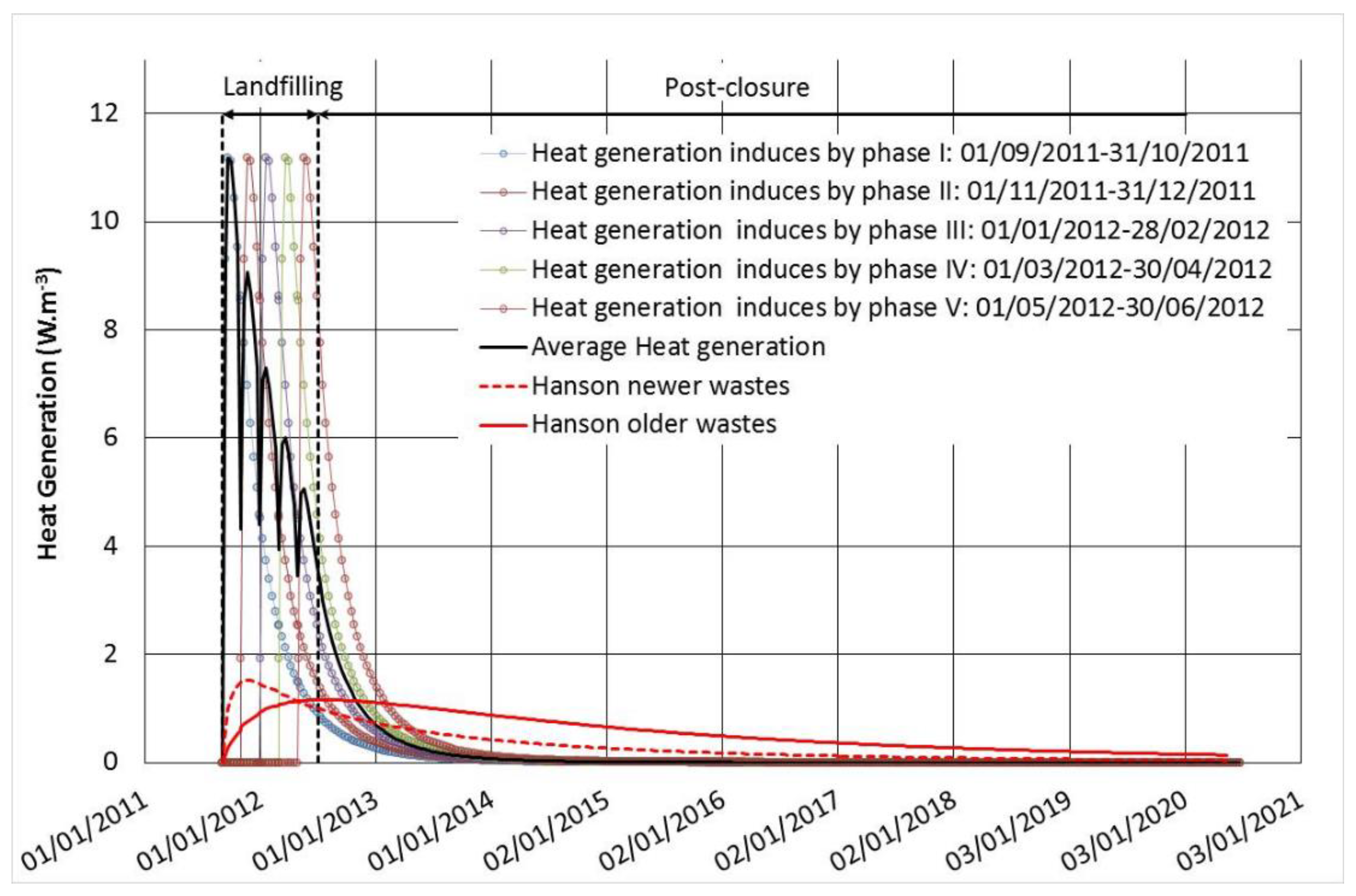
2.3.4. Heat Source Optimisation

In the literature, information is available on the thermal properties of waste, but little about the heat source (Q in W.m−3), which depends on different parameters such as biological decomposition, precipitation and ambient temperature, amount of organic matter, landfilling period with aerobic and anaerobic phases, for example. All the temperature evolutions recorded in the waste mass on CELL4, from its deposit and for several years, will show a fast increase of about forty degrees over a year followed by a slow decrease. To be in agreement with these observations, we decided to apply the heat generation rate function developed by Hanson et al. [32] (p. 1996) and named H: “The function resulted in growth of heat generation rate to a peak value followed by an exponential decay”. Only the mathematical formula of the equation of the function (Equation (3)) was retained and the parameters were defined by optimization using data, geometry, materials and boundary conditions from waste deposit CELL4 of the SAS Champs-Jouault landfill presented before.
H = A ( t B t + t ) ( C t C t + t ) e t D
“Where, H is the heat generation rate (W/m3), t is the time (day), A is the peak heat generation rate factor (W/m3), Bt and Ct are the shape factors (day), and D is the decay rate factor (day)” [32] (p. 1996).
To estimate the quality of temperature modelling, 48 locations spread over the entire CELL4 were retained to compare measured data from the fibre optic device and the temperature calculated with the numerical modelling. Twenty-nine time steps are available over the period studied, between June 20, 2012 and July 11, 2016. The mathematical difference for all the datasets between the measured temperatures Tdata(t,i) and calculated temperatures Tmodel(t,i) are expressed as a percentage of the measured temperature. This average mathematical difference is presented by Equation (4).
As proposed by Hauduc et al. [40], we choose to retain the relative root mean square error (RRMSE) expressed in percentage [41]. It indicates the overall agreement between calculated and measured data and it can be used in conjunction with the Mean absolute error MAE (Equation (5)) to provide information on the prominence of outliers in the dataset [42].
RRMSE = t = 1 29 i = 1 48 ( ( T data ( t , i ) T model ( t , i ) T data ( t , i ) ) 2 29   48   100   ( % )
MAE =   1 29 48 t = 1 29 i = 1 48 | T data ( t , i ) T model ( t , i ) |
If the value of RRMSE is low, we considered that the model mathematically reproduces the measured temperature. To reach the most appropriate models compared to the measurements recorded, we combined numerous possibilities of the thermal parameters and the fours parameters of Hanson’s equation (Equation (3)). As presented above, the modelling takes into account the landfilling of CELL4 in five successive two-month (60 days) steps. The average heat production (H in Hanson’s equation, Equation (3), and Q in Equation (1)) for the cell is therefore calculated according to the following formula (Equation (6)):
0 t < 60 H ( t ) ¯ =   H ( t ) 60 t < 119 H ( t ) ¯ =   H ( t ) +   H ( t 60 ) 2 120 t < 119 H ( t ) ¯ =   H ( t ) +   H ( t 60 ) + H ( t 120 ) 3 180 t < 119 H ( t ) ¯ =   H ( t ) +   H ( t 60 ) + H ( t 120 ) + H ( t 180 ) 4 t 240 H ( t ) ¯ =   H ( t ) +   H ( t 60 ) + H ( t 120 ) + H ( t 180 ) + H ( t 240 ) 5
where, t is the number of days with t = 0 at the beginning of the landfilling, 1 September, 2011.

3. Results and Discussion

3.1. Distributed Temperature Readings from Fibre Optics Compared to Point Temperature Readings

The main goals of the continuously recorded point sensors were (i) to consider these measurements as references and to compare these data to those recorded by the fibre-optic sensors to confirm their reliability and (ii) to obtain a continuous temperature evolution at specific points located in the waste mass. Figure 6 presents the temperature evolution of point sensors T6, T7 and T9 (Layer 2) and data recorded from optical fibres FO6 and FO7 located at the same positions FO6(T6), FO6(T7) and FO7(T9) from June 2012 to December 2015. A good agreement is observed between June 2012 and January 2014 for all measuring torques (point sensor and optical fibre) with a temperature difference of less than 1 °C which confirms the quality of the data calibration recorded from optical fibres and the expected accuracy: ±0.5 °C. Then, data losses for point sensors begin to appear as well as differences of several degrees between measurements that will gradually increase. The degradation of the insulating protection between the thermistors and the connection cable of the point sensor is the hypothesis to explain the observed deviation and the poor agreement recorded from January 2014, as well as the loss of data one year later (no agreement in Figure 6). The electrical connections located in the waste mass are suspected of being damaged by humidity, compaction, corrosion and temperature, even with insulating protection. This problem can cause the cable to break and the total loss of measurement, but also a change in the resistance read at the terminals of the thermistor sensor and lead to a completely false measurement. This can be observed for the T9 probe, which increases from 2015 onwards to a temperature of 70 °C in an inconsistent way.
Before continuous temperature measurements become unusable, the temperature evolution is characterised by two phases: a fast increase followed by a slow decrease. For point sensor T9, the first phase begins at the atmospheric temperature during the filling in May 2012 and rapidly increases in one year to reach a maximum of 62 °C in June 2013. For sensors T6 and T7, the evolutions are in the same order of magnitude but with maximum temperatures reached at different times: 62 °C for T6 in November 2012 and 65 °C for T7 in January 2013. These increases are related to waste hydrolysis when oxygen is consumed and induces an exothermic process. Maximum temperatures around 65 °C were recorded on CELL4, in total agreement with the temperature range described in the literature during the aerobic phase. Then, a second evolution is observed, characterised by a slow decrease in temperature that begins many months after the end of the landfilling. The waste cell is gradually filled from the bottom to the top and therefore simultaneously induces the combination of the aerobic phase on the last waste lift at the top and the anaerobic phase in the waste mass covered below. There are therefore different temperature kinetics depending on the height of the waste mass considered. The decrease in temperature is faster for T6 located closer to the side exposed to the ambient temperature than T7 and T9.

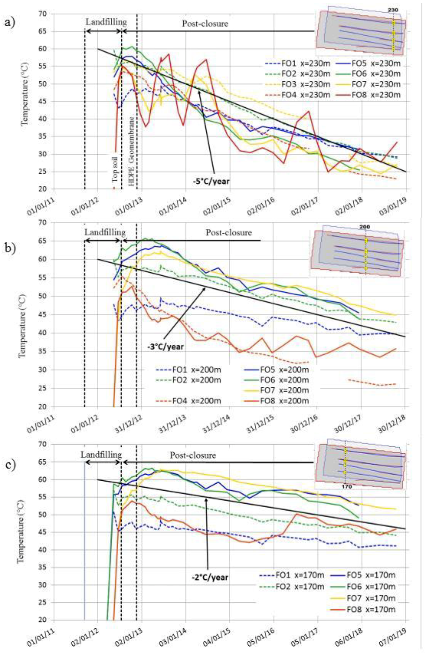
3.2. Distributed Temperatures from Fibre-Optic Sensors

The objective of the fibre-optic sensors implementation in waste body using DTS technology is to describe at a large scale the temperature distribution and its evolution over many years from the landfilling period. The optical fibres were installed on two horizontal layers and the temperature evolution is shown in Figure 7 from 2012 to 2018. The cutting planes of Layer 1 in light red and Layer 2 in light blue are shown, and we can observe that these surfaces are largely described by temperature measurements. The study of these data allows several findings.
Whatever the date for which the temperatures recorded are compared, we can see that the upper level 9 m from the bottom of the waste cell (Layer 2) is always warmer than the lower level at 4 m (Layer 1). As already mentioned, the filling process in CELL4 is from the bottom to the top and during this period (September 2011–July 2012), the waste lift at the top is in aerobic condition with a higher temperature than the waste mass below it, which is in an anaerobic condition until it is covered by another waste layer. The evolution of the waste mass temperature is also influenced by the boundary conditions of CELL4: air-soil temperature on the top and the sides not covered by another waste cell, the bottom in contact with the ground and one side leaning against CELL3 (illustrated in Figure 1b). The influence of the external climatic conditions on the waste mass temperature in a MSW landfill is classical and was clearly reported by Yesiller et al. [43] with a main impact on the sides of the waste body. For the two horizontal sections (Layer 1 and Layer 2), the highest temperatures are recorded at the centre of the surfaces studied. Although waste mass is still considered as a heterogeneous porous medium, temperature is an intensive variable controlled by the local environment and data observed do not reflect this heterogeneity: a very hot zone is located in its middle and the temperature decreases approaching the edges, influenced by the boundaries in contact with the top soil, external temperature or the surrounding waste cell, CELL3. This temperature distribution is similar to that described by Yesiller et al. [44] for the cold climate with an average ambient temperature equal to 12 °C with a minimum of −6 °C and a maximum of 27 °C, and an average annual rainfall of 1200 mm, between 2012 and 2016. No temperature discontinuity is observed, and if areas with a different thermal evolution exist, they are too small to be detected by the resolution of the temperature measurements. It could also be imagined that the thermal conductivity of the waste body around these areas is significant and sufficient to homogenise the temperature in such places. The south side of CELL4 is the most exposed to external conditions, as shown in Figure 7, with the average temperature decreasing from 50 °C to 25 °C between 2012 and 2018. From 2016, the west side is also strongly impacted by the temperature drops, but mainly at the bottom of the cell, as shown by the data on Layer 1. The external side of waste deposit CELL4 on the north is several tens of meters from the first available measurements and the influence of external conditions is not perceptible there. As presented for the boundary conditions of the numerical modelling, the east side of CELL4 is based on CELL3 and this set is considered to be in thermal equilibrium: this is confirmed by temperature measurements of the two layers that do not highlight the influence of external temperatures. As explained in the introduction, the temperature range between 35 °C and 55 °C is suitable for the bacterial population responsible for methanisation. The location of these two isotherms is shown in Figure 7 by a red line for 35 °C and a blue line for 55 °C. Temperatures above 55 °C were recorded for Layer 1 until the end of 2014 and until the end of 2016 for Layer 2, i.e., more than four years after the installation of the top barrier.
These illustrations make it possible to clearly distinguish the decrease over time of the optimal temperature zone for the methanogenic biodegradation for both levels. The evaluation of the volume representing this optimal temperature is not easy because the distribution of the measurements is not symmetrical, as well as the edge effects. However, we can already conclude that the sides of a landfill exposed to climatic conditions are only for a few years, three to four years, under optimal temperature conditions to promote the methanogenesis. In the coming years, it will be interesting to compare the evolution of the temperatures on the south and west sides of CELL4 and the average ambient temperatures recorded on the landfill site.
To continue the analysis of temperature measurements recorded from the DTS device, specific measurement points extracted from the optical at the abscissa: x = 170 m, x = 200 m, and x = 230 m, (3 dotted lines in black in Figure 2c) were studied. Data from Layer 1 (FO1, FO2, FO3 and FO4) are represented by dotted lines and those of Layer 2 (FO5, FO6, FO7 and FO8) by solid lines in Figure 8a–c.
The analysis begins with the measurement points located at x = 230 m (for FO1 to FO8, Figure 8a) which are influenced by the external conditions from the south side, as shown in the previous results. Between the end of the landfilling period in July 2012 and the implementation of HDPE Geomembrane at the top in November 2012, all temperatures are maximum and range from 53 to 60 °C, except for FO1 lower and equal to 47 °C. From 2013, the decrease is constant and identical for all measurement points, except for FO1, which decreases more slowly. In 2018, all values converge towards a narrow temperature range of 23 to 30 °C. The temperature decrease can be estimated at −5 °C per year (black line in Figure 8a) for all measurement points near the south side of CELL4, except for FO1 more in the centre of the waste cell but with an initial temperature lower than the others. The FO8 measurement point is the closest to the south side and undergoes the seasonal temperature variations with maximum in summer and minimum in winter.
For the measurement points located at x = 200 m (for FO1 to FO8, except FO3, Figure 8b), the temperatures after landfilling are the same as for x = 230 m, between 50 and 60 °C, but the maximum temperatures are reached in April/May 2013, around 57–66 °C. For Layer 1 (FO1, FO2 and FO4) and from mid-2013, temperatures decrease at the same rate with maximums recorded in the centre of the waste mass for FO2. For all data points, except for FO4 and FO8 which are highly influenced by external conditions, temperatures decrease in the same way to reach 40–45 °C in 2018, with an average trend estimated at −3 °C per year (black line in Figure 8b).
For points x = 170 m except for FO3 and FO4 for which the optical fibres are too short (Figure 8c), the previous conclusions apply: a maximum is recorded in April/May 2013, Layer 1 temperatures are lower than Layer 2 with higher values in the centre, and all Layer 2 temperatures decrease at the same rate. The temperatures reached in 2018 are between 40 and 50 °C with an average decrease of −2 °C per year (black line in Figure 8c).
Whatever the analysis considered among the optical fibres studied, an increase in temperature is observed starting during the filling operation and reaches the maximum value around 65 °C in April/May 2013, six months after the HDPE Geomembrane deposit at the top of the waste body and one year after the waste mass landfilled where the data are recorded.
This increase is linked to aerobic biodegradation before an anaerobic phase and a decrease in temperature during the post-closure period characterised by methanogenic biodegradation composed of approximately 60% methane for biogas production [45,46].
In 2018, the waste mass temperature in the heart of CELL4 is between 40 and 50 °C while the sides exposed to external climatic conditions are around 25–35 °C. The optimal temperature continues to be debated, even though Rees [6] identified the temperature range of 40–45 °C to be the optimum range for gas production at a landfill located in a temperate climate [6,47]. Generally, a temperature between 35 °C (mesophilic condition) and 55 °C (thermophilic condition) is considered to be suitable for methane production but with different kinetics due to anaerobic consortia, which differ for the two conditions [48].
The objectives of modelling as-proposed are to find the optimal thermal parameters to fit the measured temperature, to discuss these results according the operational conditions of landfilling and to predict the temperature evolution for the next years to understand if CELL4 will be under temperature conditions appropriate for methanogenic biodegradation.

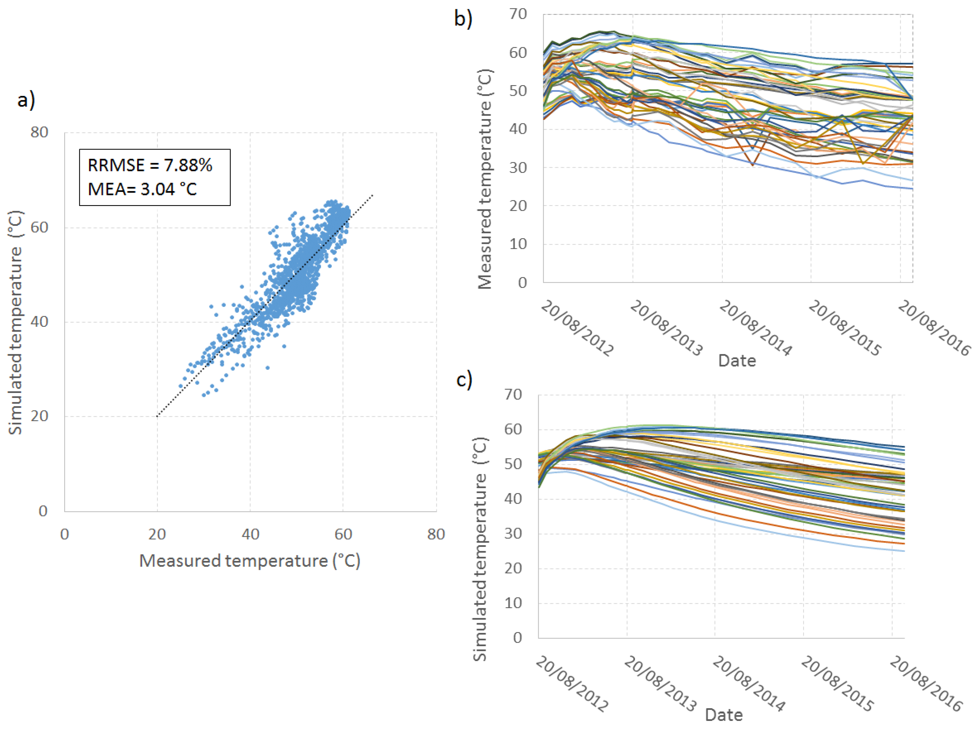
3.3. Modelling CELL4’s Temperature

The first objective of numerical modelling is to determine the thermal properties of the model and the parameters of the heat source according to Hanson’s equation (Equation (3)).
Among the thousands of simulations tested, the best fitting mathematical model was obtained for the parameters described in Table 2 and gave the following quality results: RRMSE = 7.9% and MAE = 3.0 °C (Equations (4) and (5)). Several models have a RRMSE less than 10% with parameters close to the optimal results.
The thermal conductivity of the waste mass and the soil are lower than those identified in the literature, while the results for specific heat capacity are in the known ranges. Similarly, the parameters calculated for Hanson’s equation are quite different from those found by the author in 2013. The main difficulty of our simulation was to test a large number of parameters (10 in total without counting the densities whose values were known), multiplying all possible combinations. The optimization of this simulation could be to evaluate at laboratory scale the thermal parameters of the waste mass and the soil to determine their values.
The optimal heat function presented in Figure 9 shows a peak heat generation rate value of 11.2 W.m−3 and a time for peak value equal to 20 days for each phase. These results are different from Hanson’s results (2013), who found for Cell B (older wastes) and Cell D (newer wastes) respectively, values equal to 1.16 W.m−3 and 1.52 W.m−3 for the peak heat generation rate value and to 360 days and 87 days for duration for the peak value, which represents an amplitude ten times lower and reached much later. Several hypotheses are proposed to explain this difference: the composition of the waste mass with a more important putrescible fraction, 25% in our case against 10% for Hanson, the ambient conditions with ambient temperature between −6 °C and 27 °C higher and an annual average rainfall of 1200 mm against 800 mm for Hanson. Our conditions are conducive to heat generation in the aerobic biodegradation phase with a bigger quantity of biodegradable fraction with a higher moisten waste mass and with 33% increase in rainfall.
According to Figure 9, the calculation of the total energy expended from September 2011 (beginning of landfilling CELL4) to July 2021 (3591 days later) for our optimized simulation and Hanson’s function found a total energy expended of 222 MJ/m3 in our case against 100 MJ/m3 for the older waste curve and 160 MJ/m3 for the newest waste curve. Our result is higher but in accordance with the differences presented above.
The measured and simulated temperatures are represented on a time scale in Figure 10b,c respectively, with 48 results (one colour for each result) for each of the 29 time steps.
In Figure 10a, the correlation between the measured and simulated values is presented as well as the results of RRMSE and MAE describing the quality of the optimal model. Temperatures measured below 50 °C are reduced by the model, unlike higher values, which are increased.
The modelling also shows a temperature rise of a few weeks for all points, with a shift in the maximum value reached for simulated data compared to the measured data (Figure 11). Moreover, the ranges of temperature are greater at the beginning of the simulation. In 2012, the measured data were between 42 °C and 60 °C against 43 °C and 53 °C for the simulated data. In 2016, after four years of post-closure, the temperature variation ranges were identical for measured and simulated values respectively, ranging from 25 °C to 57 °C and 25 °C to 55 °C. Despite taking into account the landfilling of the waste deposit cell from the bottom to the top modelled in 5 steps, the temperatures are not rigorously simulated in the model. Even if the model has imperfections, the results make it possible to predict future temperature changes at different points in the waste mass CELL4.
The second objective of modelling is to predict the changes in temperature spatially, more particularly, in the core of CELL4 where they are greatest. This requires that the temperature conditions applied be the same as before: 12.5 °C for soil at the bottom of the waste, ambient temperature between −6 and 27 °C, depending on the season, as in Figure 5, and on the other sides, except for the side in contact with CELL3, where thermal equilibrium is preserved with CELL4. As stated above, the temperature conditions will be favourable for biodegradation methanogenesis as long as temperature will be higher than 35 °C and modelling predicts that the heart of the waste mass, where the temperature is highest, will reach this value in 2025, thirteen years after the beginning of the simulation (Figure 11). This duration is in accordance with the decrease of −2 °C/year evaluated with the temperature measured in Figure 8c for the slower temperature decrease: 60 °C in January 2012 allows for calculating a temperature of 35 °C, 12.5 years later in July 2024. Before that date, after four or five years depending the layer considered, the situation is already much less appropriate for waste surrounding the middle of the waste body, especially near the sides, which represents a large amount of waste mass. This difficulty of keeping the waste cell sides at optimal temperature is also reinforced by the fact that these locations are more difficult to moisten, one of the key parameters for biodegradation, with leachate recirculation networks implanted mainly at the middle and the top of the waste cell. For the landfill operator, this information is very important, because the Champs-Jouault site heats the leachates before recirculation on waste deposit cell and after many years, the injection of warm leachate could allow to maintain an optimal temperature to promote the biodegradation processes.

4. Conclusions

Irstea has been conducting a research program with the bioreactor landfill operator SAS Les Champs Jouault since 2011 to study the evolution of waste biodegradation at the landfill scale with numerous measurements taken inside the waste mass. Among all the sensors used, 1200 m of optical fibres using with distributed temperature sensing technology were installed at different layers in waste CELL4 and continue to be operational. Mechanical protection was provided with sand and geotextile on both sides of the sensors for protection. Only the connection between the fibre optic and the DTS equipment is fragile and requires careful handling. One technical difficulty, regarding the distributed temperature sensing technology using fibre-optic sensors in MSW landfills is the setting up of the sensors which must be in contact with the waste mass. However, the temperature calibration is easy, and when performed automatically at each measurement can allow for a temperature uncertainty of ±0.5 °C. Moreover, and perhaps one of the most important aspects with temperature studies, is that data interpretation is simple.
The temperature distribution in waste CELL4 shows us that it performs thermally as a single-block, whose evolution follows the same trend but with different temperatures depending on the location of the measuring points: warmer in the centre and colder on the sides.
The waste mass is at ambient temperature when it arrives on the landfilling cell and its temperature quickly rises in less than one year to reach maximum temperatures of 60–65 °C. This phase begins during the landfilling aerobic phase (starting in September 2011) and ends for the last fraction of waste mass stored (July 2012) during the post-closure phase. After these maximum temperatures have been reached, the temperatures decrease slowly and the rate of decrease is strongly impacted by the effects of the external conditions on the sides of the waste cell. In July 2018, six years after the maximum temperatures, the heart of the waste mass which is still the warmest, is around 45–50 °C and the measuring points closest to the edges are around 25 °C. The heterogeneity of the waste mass does not show up in the temperature variations and for the temperature survey, the waste can be considered as a single unit.
The temperature simulation manages to predict its evolution over time to check if the waste mass will be in suitable temperature conditions, between 35 °C and 55 °C, to promote methanogenesis biodegradation. The temperature simulation found the most suitable thermal parameters and parameter for Hanson’s equation to fit the measured temperature. The quality of results of the simulation (RRMSE and MAE), demonstrate the robustness of the model even if the thermal parameters calculated for waste mass and soil as well as the parameters of Hanson’s equation are not identical to those identified in the literature. Over the simulation period, 2012 to 2016, the differences between the measured and simulated values are greater at the beginning than at the end, even with the layered landfilling being taken into account. As it was clarified before, heat waste generation and its transfer are largely influenced by waste composition and mechanical characteristics, precipitation and ambient temperature, amount of organic matter, and landfilling period with aerobic and anaerobic phases, for example. The landfill studied is therefore characterised by a higher heat production in a very short time compared to the sites identified in the literature. The simulation calculates a four-year period for the edges of the CELL4, and a thirteen-year period for the entire waste mass, to be at a temperature below 35 °C after landfilling. For an industrial operator, knowing the temperature evolution for the coming years is important to manage a landfill in a bioreactor mode.
To conclude, temperature measurement in landfill at a large scale is an essential physical parameter to study, because its relation to promote the different biodegradation phases is well known and very often studied at a laboratory scale.

Author Contributions

Resources, T.J. and J.G.-D.; Software, R.C.; Conceptualization, R.C.; Project administration, S.M. and S.L.; Supervision, L.M. and R.C.; Validation, S.M.; Writing–original draft, L.M. and R.C.; Writing–review and editing, S.M.

Funding

This research was funded by FEDER and the “Région Basse Normandie”.

Acknowledgments

The authors would like to thank Guthi Raja-Sekhar (Irstea Lyon, France) in particular for his review of the entire document.

Conflicts of Interest

The authors declare no conflict of interest. The funders had no role in the design of the study; in the collection, analyses, or interpretation of data; in the writing of the manuscript, or in the decision to publish the results.

References

  1. Eurostat. Treatment of Waste by Waste Category, Hazardousness and Waste Operations. Available online: http://appsso.eurostat.ec.europa.eu/nui/submitViewTableAction.do. (accessed on 1 October 2019).
  2. Barlaz, M.A.; Reinhart, D. Bioreactor landfills: Progress continues. Waste Manag. 2004, 24, 859–860. [Google Scholar] [CrossRef] [PubMed]
  3. Imhoff, P.T.; Reinhart, D.R.; Englund, M.; Guérin, R.; Gawande, N.; Han, B.; Jonnalagadda, S.; Townsend, T.G.; Yazdani, R. Review of state of the art methods for measuring water in landfills. Waste Manag. 2007, 27, 729–745. [Google Scholar] [CrossRef] [PubMed]
  4. Reinhart, D.R.; Townsend, T.G. Landfill Bioreactor Design & Operation; Lewis Publishers: Boca Raton, FL, USA, 1997. [Google Scholar]
  5. Pohland, F.G.; Al-Yousfi, B. Design and operation of landfills for optimum stabilization and biogas production. Water Sci. Technol. 1994, 30, 117–124. [Google Scholar] [CrossRef]
  6. Rees, J.F. The fate of carbon compounds in the landfill disposal of organic matter. J. Chem. Technol. Biotechnol. 1980, 30, 161–175. [Google Scholar] [CrossRef]
  7. Reinhart, D.; Al-Yousfi, B. The Impact of leachate recirculation on municipal solid waste landfill operating characteristics. Waste Manag. Res. 1996, 14, 337–346. [Google Scholar] [CrossRef]
  8. Arrêté du 15 Février 2016 Relatif aux Installations de Stockage de Déchets non Dangereux. Available online: https://www.legifrance.gouv.fr/eli/arrete/2016/2/15/DEVP1519168A/jo/texte (accessed on 1 October 2019).
  9. Rendra, S.; Warith, M.; Fernandes, L. Degradation of Municipal Solid Waste in Aerobic Bioreactor Landfills. Environ. Technol. 2007, 28, 609–620. [Google Scholar] [CrossRef]
  10. Warith, M. Bioreactor landfills: experimental and field results. Waste Manag. 2002, 22, 7–17. [Google Scholar] [CrossRef]
  11. Christensen, T.H.; Kjeldsen, P. Basic biochemical processes in landfills. In Sanitary Landfill: Process, Technology, and Environmental Impact; Christensen, T.H., Cossu, R., Stegman, R., Eds.; Academic Press: London, UK, 1989. [Google Scholar]
  12. Augenstein, D.; Pacey, J. Modeling landfill methane generation. In Proceedings of the Third International Landfill Symposium, Sardinia, Italy, 14–18 October 1991; pp. 115–148. [Google Scholar]
  13. Aguilar-Juarez, O. Analyse et Modélisation des Réactions Biologiques Aérobies au Cours de la Phase D’exploitation d’un Casier d’un Centre D’enfouissement Technique. Ph.D. Thesis, Institut des Sciences Appliquées de Toulouse, Toulouse, France, 21 June 2000. [Google Scholar]
  14. Tchobanoglous, G.; Theisen, H.; Vigil, S.A. Integrated Solid Waste Management: Engineering Principles and Management Issues; McGraw-Hill: New York, NY, USA, 1993. [Google Scholar]
  15. El-Fadel, M.; Findikakis, A.N.; Leckie, J.O. Estimating and Enhancing Methane Yield from Municipal Solid Waste. Hazard. Waste Hazard. Mater. 1996, 13, 309–331. [Google Scholar] [CrossRef]
  16. Batstone, D.J.; Keller, J.; Angelidaki, I.; Kalyuzhnyi, S.V.; Pavlostathis, S.G.; Rozzi, A.; Sanders, W.T.M.; Siegrist, H.; Vavilin, V.A. Anaerobic digestion model No 1 (ADM1). Water Sci. Technol. 2002, 45, 65–73. [Google Scholar] [CrossRef]
  17. Aghdam, E.F.; Scheutz, C.; Kjeldsen, P. Assessment of methane production from shredder waste in landfills: The influence of temperature, moisture and metals. Waste Manag. 2017, 63, 226–237. [Google Scholar] [CrossRef] [Green Version]
  18. Gawande, N.A.; Reinhart, D.R.; Thomas, P.A.; McCreanor, P.T.; Townsend, T.G. Municipal solid waste in situ moisture content measurement using an electrical resistance sensor. Waste Manag. 2003, 23, 667–674. [Google Scholar] [CrossRef]
  19. Kumar, S.; Bhattacharyya, J.; Vaidya, A.; Chakrabarti, T.; Devotta, S.; Akolkar, A. Assessment of the status of municipal solid waste management in metro cities, state capitals, class I cities, and class II towns in India: An insight. Waste Manag. 2009, 29, 883–895. [Google Scholar] [CrossRef] [PubMed]
  20. Moreau, S.; Ripaud, F.; Saidi, F.; Bouyé, J.-M. Laboratory test to study waste moisture from resistivity. Proc. Inst. Civ. Eng. Waste Resour. Manag. 2011, 164, 17–30. [Google Scholar] [CrossRef]
  21. Bernstone, C.; Dahlin, T.; Ohlsson, T.; Hogland, H. DC-resistivity mapping of internal landfill structures: Two pre-excavation surveys. Environ. Earth Sci. 2000, 39, 360–371. [Google Scholar] [CrossRef]
  22. Gazoty, A.; Fiandaca, G.; Pedersen, J.; Auken, E.; Christiansen, A. Gazoty Mapping of landfills using time-domain spectral induced polarization data: the Eskelund case study. Near Surf. Geophys. 2012, 10, 575–586. [Google Scholar] [CrossRef]
  23. Leroux, V.; Dahlin, T.; Svensson, M. Dense resistivity and induced polarization profiling for a landfill restoration project at Härlöv, Southern Sweden. Waste Manag. Res. 2007, 25, 49–60. [Google Scholar] [CrossRef]
  24. Ettala, M.; Sormunen, K.; Englund, M.; Hyvönen, P.; Laurila, T.; Karhu, K.; Rintala, J. Instrumentation of a landfill. In Proceedings of the 9th International Waste Management and Landfill Symposium, Cagliari, Italy, 6–10 October 2003; pp. 199–200. [Google Scholar]
  25. Moreau, S.; Chevrier, B.; Saidi, F.; Buton, G.; Bouye, J.-M. Using fibreoptic to measure waste mass temperature: Application to evaluate leachate recirculation network in landfill bioreactor. In Proceedings of the Sardinia 2009 Twelfth International Waste Management and Landfill Symposium, Sardinia, Italy, 5–9 October 2009. [Google Scholar]
  26. Gholamifard, S. Modélisation des Écoulements Diphasiques Bioactifs Dans les Installations de Stockage de Déchets. Ph.D. Thesis, Université Paris Est Marne La Vallée, Champs-sur-Marne, France, January 2009. [Google Scholar]
  27. Faitli, J.; Magyar, T.; Erdélyi, A.; Murányi, A. Characterization of thermal properties of municipal solid waste landfills. Waste Manag. 2014, 36, 213–221. [Google Scholar] [CrossRef]
  28. Yesiller, N.; Hanson, J.L.; Yee, E.H. Waste heat generation: A comprehensive review. Waste Manag. 2015, 42, 166–179. [Google Scholar] [CrossRef] [Green Version]
  29. Faitli, J.; Magyar, T.; Romend, R.; Erdélyi, A.; Boldizsár, C. Laying the Foundation for Engineering Heat Management of Waste Landfills. In Landfills: Environmental Impacts, Assessment and Management; Chandler, N., Ed.; Nova Science Publishers: Hauppauge, NY, USA, 2017; Chapter 9; pp. 215–244. [Google Scholar]
  30. Lefebvre, X.; Lanini, S.; Houi, D. The role of aerobic activity on refuse temperature rise, I. Landfill experiment study. Waste Manag. Res. 2000, 18, 444–452. [Google Scholar] [CrossRef]
  31. Hanson, J.L.; Yesiller, N.; Oettle, N.K. Spatial Variability of Waste Temperatures in MSW Landfills. In Proceedings of the Global Waste Management Symposium, Phoenix, AZ, USA, 24–28 February 2008. [Google Scholar]
  32. Hanson, J.L.; Yesiller, N.; Onnen, M.T.; Liu, W.-L.; Oettle, N.K.; Marinos, J.A. Development of numerical model for predicting heat generation and temperatures in MSW landfills. Waste Manag. 2013, 33, 1993–2000. [Google Scholar] [CrossRef] [Green Version]
  33. European Committee for Standardization. BS EN 14899 Characterization of Waste. Sampling of Waste Materials. Framework for the Preparation and Application of a Sampling Plan; Deutsches Institut für Normung: Berlin, Germany, 2006. [Google Scholar] [CrossRef]
  34. Déchets Ménagers et Assimilés–Méthode de caractérisation–Analyse sur Produit sec NF X30-466; French Standardization Association: Paris, France, 2013.
  35. ADEME Éditions. La Composition des Ordures Ménagères en France; ADEME Éditions: Montpellier, France, 2010; ISBN 978-2-35838-093-5. [Google Scholar]
  36. Perry, R.H.; Green, D.W. Perry’s Chemical Engineers’ Handbook; McGraw-Hill: New York, NY, USA, 1997. [Google Scholar]
  37. Audebert, M.; Oxarango, L.; Duquennoi, C.; Touze-Foltz, N.; Forquet, N.; Clément, R. Understanding leachate flow in municipal solid waste landfills by combining time-lapse ERT and subsurface flow modelling-Part II: Constraint methodology of hydrodynamic models. Waste Manag. 2015, 55, 176–190. [Google Scholar] [CrossRef] [PubMed]
  38. Bonany, J.; Van Geel, P.J.; Gunay, H.B.; Isgor, O.B. Heat budget for a waste lift placed under freezing conditions in a landfill operated in a northern climate. Waste Manag. 2013, 33, 1215–1228. [Google Scholar] [CrossRef] [PubMed]
  39. Audebert, M.; Clement, R.; Moreau, S.; Duquennoi, C.; Loisel, S.; Touze-Foltz, N. Understanding leachate flow in municipal solid waste landfills by combining time-lapse ERT and subsurface flow modelling—Part I: Analysis of infiltration shape on two different waste deposit cells. Waste Manag. 2016, 55, 165–175. [Google Scholar] [CrossRef] [PubMed]
  40. Hauduc, H.; Neumann, M.; Muschalla, D.; Gamerith, V.; Gillot, S.; Vanrolleghem, P.; Vanrolleghem, P. Efficiency criteria for environmental model quality assessment: A review and its application to wastewater treatment. Environ. Model. Softw. 2015, 68, 196–204. [Google Scholar] [CrossRef]
  41. Willmott, C.J.; Ackleson, S.G.; Davis, R.E.; Feddema, J.J.; Klink, K.M.; Legates, D.R.; O’Donnell, J.; Rowe, C.M. Statistics for the evaluation and comparison of models. J. Geophys. Res. 1985, 90, 8995–9005. [Google Scholar] [CrossRef] [Green Version]
  42. Bennett, N.D.; Croke, B.F.W.; Guariso, G.; Guillaume, J.H.A.; Hamilton, S.H.; Jakeman, A.J.; Marsili-Libelli, S.; Newham, L.T.H.; Norton, J.P.; Perrin, C.; et al. Characterising performance of environmental models. Environ. Model. Softw. 2013, 40, 1–20. [Google Scholar] [CrossRef]
  43. Yesiller, N.; Hanson, J.L.; Liu, W.-L. Heat Generation in Municipal Solid Waste Landfills. J. Geotech. Geoenviron. Eng. 2005, 131, 1330–1344. [Google Scholar] [CrossRef] [Green Version]
  44. Yeşiller, N.; Hanson, J.L.; Kopp, K.B.; Yee, E.H. Heat management strategies for MSW landfills. Waste Manag. 2016, 56, 246–254. [Google Scholar] [CrossRef] [Green Version]
  45. Barlaz, M.A.; Ham, R.K.; Schaefer, D.M.; Isaacson, R. Methane production from municipal refuse: A review of enhancement techniques and microbial dynamics. Crit. Rev. Environ. Control. 1990, 19, 557–584. [Google Scholar] [CrossRef]
  46. Farquhar, G.J.; Rovers, F.A. Gas production during refuse decomposition. Water Air Soil Pollut. 1973, 2, 483–495. [Google Scholar] [CrossRef]
  47. Rees, J.F. Optimisation of Methane Production and Refuse Decomposition in Landfills by Temperature Control. J. Chem. Technol. Biotechnol. 1980, 30, 458–465. [Google Scholar] [CrossRef]
  48. Karakashev, D.; Batstone, D.J.; Angelidaki, I. Influence of Environmental Conditions on Methanogenic Compositions in Anaerobic Biogas Reactors. Appl. Environ. Microbiol. 2005, 71, 331–338. [Google Scholar] [CrossRef] [PubMed] [Green Version]
Figure 1. (a) Location of the experimental site, (b) aerial photograph of the industrial site, (c) geometry of experimental waste deposit cell CELL4, (d) internal geometry of the waste deposit CELL4 and (e) mixed biogas collection and leachate recirculation pipe in a horizontal trench.
Geosciences 09 00426 g001
Figure 2. (a) Picture, (b) three-dimensional (3D) exploded view of experimental CELL4 and (c) Layer 1 and Layer 2 on CELL4 for the temperature distribution study.
Geosciences 09 00426 g002
Figure 3. Evolution of the waste geometry over time: (a) 0 to 59 days, (b) 60 to 119 days, (c) 120 to 179 days, (d) 180 to 239 days and (e) 240 to the end.
Geosciences 09 00426 g003
Figure 4. Geometry and boundary conditions of waste deposit CELL4: (a) distribution of the material properties (① waste; ② loam soil), (b,c) boundary conditions (③ air temperature in red; ④ average soil temperature in green; ⑤ symmetry boundary in purple).
Geosciences 09 00426 g004
Figure 5. Daily evolution of the ambient air temperature during five seasons.
Geosciences 09 00426 g005
Figure 6. Evolution of point sensor T6, T7 and T9 and data recorded from optical fibres FO6 and FO7 at the same position.
Geosciences 09 00426 g006
Figure 7. Evolution of interpolated temperature distribution recorded with Distributed Temperature Sensing (DTS) technology in waste CELL4 for Layer 1 and Layer 2.
Geosciences 09 00426 g007
Figure 8. Evolution of specific measurement points from optical fibres lines: (a) x = 230 m, (b) x = 200 m and (c) x = 170 m.
Geosciences 09 00426 g008
Figure 9. Heat generation evolution during the landfilling and post closure periods for CELL4 and for Hanson’s data [32].
Geosciences 09 00426 g009
Figure 10. (a) Distribution of measured and simulated temperature for the same data points, (b) evolution of measured temperature and (c) evolution of simulated temperature.
Geosciences 09 00426 g010
Figure 11. Simulation of CELL4 temperature evolution until 2030 for Layer 1 and Layer 2.
Geosciences 09 00426 g011
Table 1. Thermal properties for the medium studied.
Density
(kg.dm−3)
Thermal Conductivity
(W.m−1.K−1)
Specific Heat Capacity
(J.kg−1.K−1)
Soil (loamy soil)1.50.35–12300–2500
Waste mass0.950.10–0.501500–2500
Table 2. Thermal properties for best fitting modelling.
Density
(kg.dm−3)
Thermal Conductivity
(W.m−1.K−1)
Specific Heat Capacity
(J.kg−1.K−1)
Soil (loamy soil)1.50.352400
Waste mass0.950.211800
Best fitting parameters for Hanson’s function (Equation (2)).
A = 100 (W/m3)B = 40 (day)C = 500 (day)D = 18 (day)

