Assessment of CO2 Injectivity During Sequestration in Depleted Gas Reservoirs


1
Division of Physical Science and Engineering, King Abdullah University of Science and Technology, KAUST, Building 5/3221, Thuwal 23955-6900, Saudi Arabia
2
Laboratoire d’Hydrologie et Geochemie de Strasbourg, University of Strasbourg/ENGEES/CNRS, 67084 Strasbourg, France
3
Departments of Geology and Environmental Engineering, University of Cincinnati, Cincinnati, OH 45221, USA
*
Author to whom correspondence should be addressed.
Geosciences 2019, 9(5), 199; https://0-doi-org.brum.beds.ac.uk/10.3390/geosciences9050199
Submission received: 3 April 2019
/
Revised: 14 April 2019
/
Accepted: 18 April 2019
/
Published: 5 May 2019
Abstract
:Depleted gas reservoirs are appealing targets for carbon dioxide (CO) sequestration because of their storage capacity, proven seal, reservoir characterization knowledge, existing infrastructure, and potential for enhanced gas recovery. Low abandonment pressure in the reservoir provides additional voidage-replacement potential for CO and allows for a low surface pump pressure during the early period of injection. However, the injection process poses several challenges. This work aims to raise awareness of key operational challenges related to CO injection in low-pressure reservoirs and to provide a new approach to assessing the phase behavior of CO within the wellbore. When the reservoir pressure is below the CO bubble-point pressure, and CO is injected in its liquid or supercritical state, CO will vaporize and expand within the well-tubing or in the near-wellbore region of the reservoir. This phenomenon is associated with several flow assurance problems. For instance, when CO transitions from the dense-state to the gas-state, CO density drops sharply, affecting the wellhead pressure control and the pressure response at the well bottom-hole. As CO expands with a lower phase viscosity, the flow velocity increases abruptly, possibly causing erosion and cavitation in the flowlines. Furthermore, CO expansion is associated with the Joule–Thomson (IJ) effect, which may result in dry ice or hydrate formation and therefore may reduce CO injectivity. Understanding the transient multiphase phase flow behavior of CO within the wellbore is crucial for appropriate well design and operational risk assessment. The commonly used approach analyzes the flow in the wellbore without taking into consideration the transient pressure response of the reservoir, which predicts an unrealistic pressure gap at the wellhead. This pressure gap is related to the phase transition of CO from its dense state to the gas state. In this work, a new coupled approach is introduced to address the phase behavior of CO within the wellbore under different operational conditions. The proposed approach integrates the flow within both the wellbore and the reservoir at the transient state and therefore resolves the pressure gap issue. Finally, the energy costs associated with a mitigation process that involves CO heating at the wellhead are assessed.
1. Introduction
The ongoing accumulation of greenhouse gas (GHG) concentrations in the atmosphere from various anthropogenic sources is believed to be the primary cause of the increasing temperature of the Earth’s surface [1,2,3,4]. Carbon dioxide is the most significant GHG and the largest anthropogenic sources of CO emissions are electricity generation and stationary industry sectors powered by fossil fuels [5,6]. Among other technologies, carbon capture and storage (CCS) of CO in geological formations is expected to play a key role in addressing the urgent call by the Paris Agreement on climate change to reduce GHG emissions [7,8,9,10]. Ddriven by their superior storage potential, most of the CCS literature has focused on assessing the storage potential of deep saline formations and oil reservoirs for enhanced oil recovery (EOR). Depleted gas reservoirs exhibit smaller storage potential. However, they could be easier targets for CCS because of their known capacity, reservoir structure, rock characterization, proven containment, and existing surface facilities that could be adapted for CO storage operations. The worldwide CO storage capacity of depleted gas reservoirs is estimated to be around 390 gigatons, based on a conservative reservoir voidage replacement ratio of 60% [11]. This storage capacity is approximately ten times the world’s current annual CO emissions and could provide a practical near-term option for CO sequestration. Nevertheless, the costs associated with CO capture and transportation remain the major barrier to field deployments.
Besides the CO entrapment potential of depleted gas reservoirs, several simulation and experimental studies showed the benefits of injecting CO to enhance gas recovery [12,13,14,15]. Since CO has a higher density and viscosity than natural gas under reservoir conditions, using CO as the displacing fluid encourages low gas mixing and an efficient and stable CO–methane displacement front [16,17]. It is known that CO in its supercritical state can be stored more efficiently in subsurface formations than in its gas or liquid state. For this reason, the Joule II research study, conducted by the European Commission in 1993, concluded that shallow reservoirs are not recommended for CO sequestration as CO will be in its gas or liquid state [18,19]. In reservoirs deeper than 800 m (2600 ft), the temperature and pressure at typical hydrostatic and geothermal conditions will be high enough for CO to be in its supercritical state, which allows increased storage and entrapment. The study also concluded that depleted gas reservoirs with low abandonment pressures and weak aquifer invasion, such as some reservoirs in the North Sea, are appealing for CO sequestration as the CO storage capacity could potentially equal the extracted gas volume. Many publications on CO sequestration in depleted gas reservoirs have addressed different aspects, such as the CO flow and trapping mechanisms, storage capacity, reservoir containment, risk assessment, and geomechanics [20,21,22,23,24,25,26].
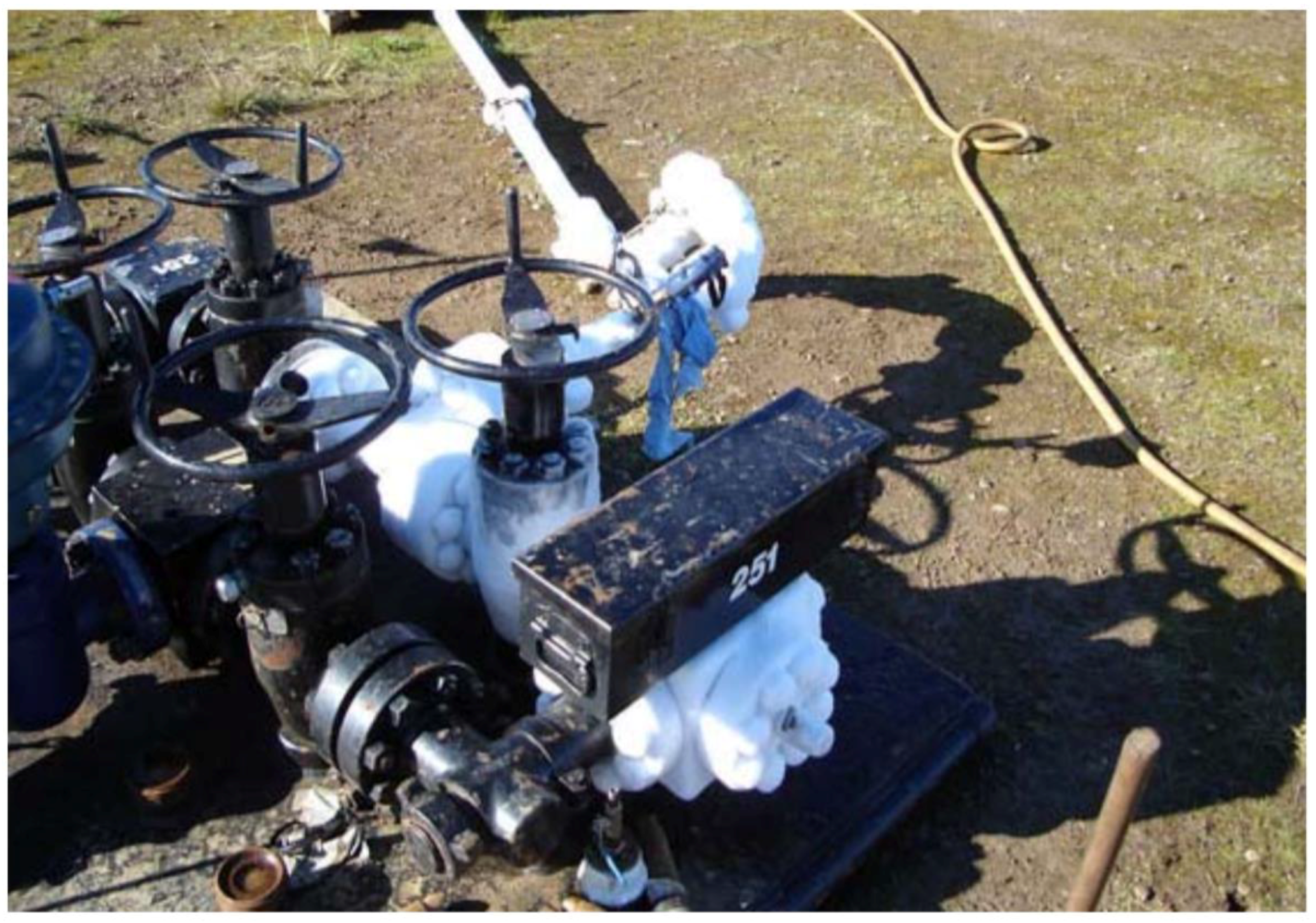
In this work, we investigate a serious flow-assurance issue that arises during CO injection into depleted gas reservoirs when the abandonment reservoir pressure is below the CO bubble-point pressure. This work is inspired by a potential CO sequestration project in a depleted gas reservoir in the North Sea [27,28]. A similar project was also recently proposed by Shell UK Limited [29]. As CO in its liquid or supercritical state is injected at surface conditions into a subsurface formation with a pore pressure lower than the bubble point, CO will surely vaporize within the well tubing or in the near-wellbore region in the reservoir. The dense-to-gas state conversion of CO is associated with several flow-assurance issues. The density of CO drops sharply by a factor of about five, which implies that the volume of the gas phase increases by the same factor. Further, the resulting gas-phase viscosity drops by a factor of about two, which boosts the mobility of the fluid. As a result, the flow velocity may increase beyond the designed erosion velocity of the flowlines. The sharp change in density may cause backpressure that impacts the well tubing-head-pressure (THP) and the reservoir bottom-hole pressure (BHP). Moreover, CO vaporization will result in a localized cooling phenomenon known as the Joule–Thomson (JT) or throttling effect [30,31,32]. Below a certain temperature, and with the presence of water and a gas (either CO or methane), a solid hydrate phase will form that can impair the CO injectivity at the well. Loss of injectivity associated with CO expansion is an operational hazard that, in some situations, could cause well integrity issues [33,34]. The JT cooling effect has been observed in the field. For instance, Xu et al. [35] reported the observation of this phenomenon at the wellhead of a CO injection well where CO was injected in its liquid state. Because of a low reservoir pressure, CO flashed to its gas state within the wellhead and the feed pipeline causing cooling and ice formation on the exterior of the system, as shown in Figure 1. Maloney and Briceno (2009) demonstrated this phenomenon in the lab by injecting CO in a slim tube at high pressure (3500 psia) while maintaining low pressure (200 psia) at the slim tube outlet. CO flashed and caused localized cooling within the slim tube that eventually resulted in hydrate formation and a complete flow blockage.
The JT cooling effect in relation to CO injection into low-pressure formations has been discussed by many authors [36,37,38]. However, few studies have investigated the transient flow behavior within the well tubing. Most existing studies assessed the conditions of CO flow in its steady state using standalone thermodynamic phase-behavior calculations and without coupling the CO flow in its steady state with the flow inside the reservoir [39,40]. Because of this decoupled steady-state approach, a discontinuity in the pressure profile was predicted within the wellbore. As we explain below, this pressure discontinuity, also referred to as the pressure gap, is unrealistic. In this work, we focus on investigating the multiphase flow behavior of CO in the wellbore under different operational conditions. We show that the pressure gap, which reflects the discontinuity between the liquid CO and gaseous CO densities, is an artifact of the steady-state assumption. Then, we introduce a new coupled approach that integrates the multiphase flow in the wellbore and the reservoir at the transient state. We show, for the first time, that CO flows in an unstable two-phase state where liquid CO and gaseous CO coexist. This flow behavior cannot be captured by a steady-state model. We also assess a mitigation process of heating CO at the wellhead.
This paper is organized as follows. First, we discuss the phase-transition issue relative to CO sequestration in depleted gas reservoirs. Next, we review the decoupled model and the resulting pressure gap. Then, we introduce our coupled model and show the synergy between the two approaches. Finally, we discuss a potential solution to mitigate the flow-assurance issue by heating CO. Note that we use field units in the analysis, and we refer to Lake 2007 [41] for the conversion factors to the SI metric unit.
2. CO Storage in a Depleted Gas Reservoir
The target storage site is an offshore dry gas reservoir located in the North Sea, approximately 140 km offshore. The reservoir is at a true vertical depth (TVD) of 9000 ft (2744 m) with an initial average pressure () of 4200 psia (290 bara) and temperature (T) of 182 F (84 C). The reservoir is currently abandoned at a pressure () of 200 psia (14 bara), corresponding to a recovery factor of 90% of the original gas in place. The dominant recovery mechanism is methane gas expansion. The recovery contribution from aquifer support and water drive is less than 2%. As a result, there has been very little change in the average gas saturation of the reservoir during the whole production lifecycle. The reservoir formation is clean sandstone with almost homogeneous porosity and permeability. Thus, the formation properties, capacity, and geological sealing of this reservoir are favorable for CO storage. The proposed CO sequestration plan includes capturing CO from an onshore power plant and transporting it in the dense phase via a 140 km subsea pipeline to the storage site. Technical challenges typically associated with CO sequestration in depleted gas reservoirs include drilling complications in depleted zones and well integrity, as well as CO transport, monitoring, capture, dehydration, and compression. This work focuses on the CO thermodynamics associated with the injection of either liquid or supercritical CO into a low-pressure environment and the potential injectivity issues arising from CO vaporization. The phase transition of CO from the dense state to the gas state produces temperature cooling, an increase in flow velocity, and pressure chokes that could impact wellbore integrity, wellhead control, and CO injectivity. In this study, the CO transport journey from the capture site to the storage site also entails different pressure–volume–temperature (PVT) conditions, as described in the following section.
3. CO Transport Journey
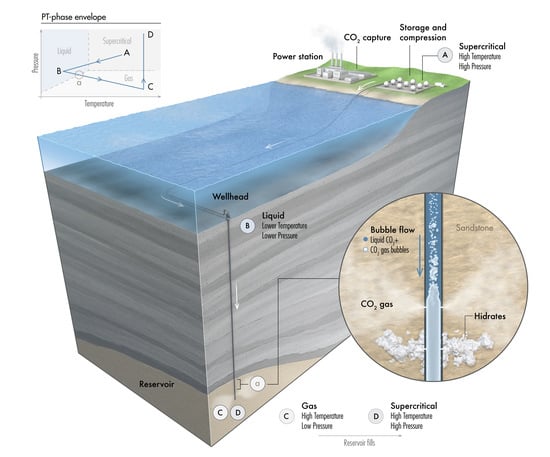
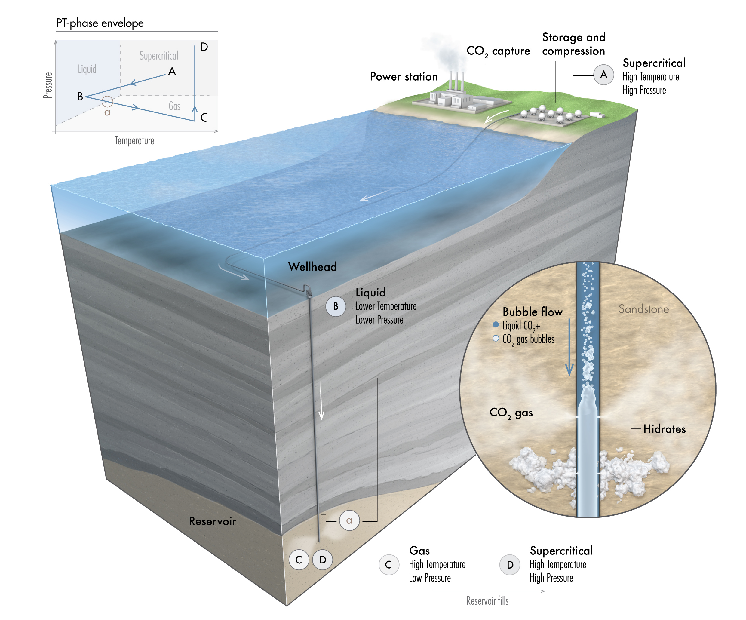
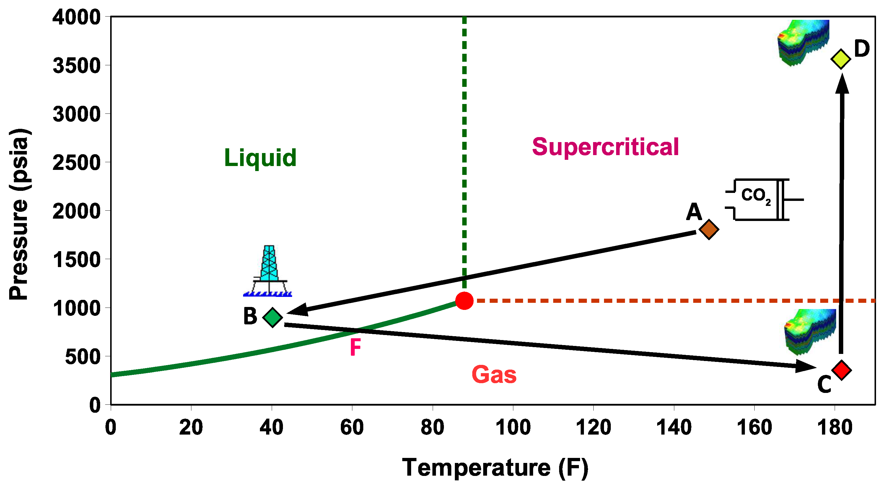
Understanding CO phase behavior and the associated PVT effects within the surface network, the wellbore, and the near-wellbore subsurface formation is crucial for successful CCS. CO can exist in solid, liquid, gas, and supercritical states. Under very low temperatures (around −109 F), CO forms dry ice, which is not expected to occur under normal CO injection conditions. When the temperature and pressure exceed a critical point ( = 1070 psia, = 87 F), CO transitions to the supercritical state. Figure 2 shows the CO pressure–temperature (PT) diagram with the PT regions corresponding to the liquid, gas, and supercritical phase states. The critical point occurs at the intersection of the three state boundaries. Because of the different PVT conditions during the capture, transportation, and injection processes, CO is likely to transition among all three states at different stages during its journey from the capture site to the storage site. In Figure 2, we superimpose the expected PT stages of CO on the phase envelope, as follows:
- Stage A: CO is captured, dehydrated, and compressed at the onshore power plant. The required delivery pressure at the compressor depends on the desired injection rate at the wellhead, the pipeline tubing diameter, and the corresponding pressure drop between the compression site and the subsurface reservoir. The pressure drop is expected to vary during the reservoir filling process, as will be discussed later. To maintain efficiency in pipeline transportation, CO must be transported and injected in the dense state. Transporting CO in the gas state is inefficient. Stage A in Figure 2 corresponds to one scenario where the pressure and temperature of CO delivered from a multistage compression unit at the onshore facility is about A = (1550 psia, 150 F).
- Stage B: This stage corresponds to the arrival conditions of CO at the wellhead. The pressure drop within the 140 km pipeline (AB) is about 550 psia, and the CO temperature is expected to adjust to the seawater temperature. The seawater temperature fluctuates between 40 F in the winter and 60F in the summer. Within that temperature range, CO is in the liquid state (Figure 2). Stage B in Figure 2 corresponds to a scenario where the pressure and temperature of CO at the wellhead is B = (1000 psia, 40 F).
- Stage C: This stage corresponds to the reservoir pressure and temperature conditions before the CO injection begins. Therefore, stage C in Figure 2 corresponds to the current reservoir conditions of C = (200 psia, 182 F). We note the liquid-to-gas (L–G) phase transition that occurs as a result of the pressure and temperature change from the surface to the reservoir. Point L–G denotes the flash point of CO. Depending on the flow and thermal conditions, the transition to a gas state may occur within the well tubing or the near-wellbore formation. Additional details are provided in the next section.
- Stage D: This stage represents the expected pressure and temperature conditions after the reservoir has been filled up with CO. We assume 100% voidage replacement, and therefore, the final pressure is expected to roughly equal the initial reservoir pressure. With no perturbation to the average reservoir temperature, stage D in Figure 2 corresponds to a supercritical state of CO at D = (3500 psia, 182 F).
It should be noted that as the pressure builds up in the reservoir due to CO filling, additional compression for CO at the wellhead could be needed to raise the reservoir pressure to its initial condition (point D), which reflects additional cost associated with the operations and offshore facility.
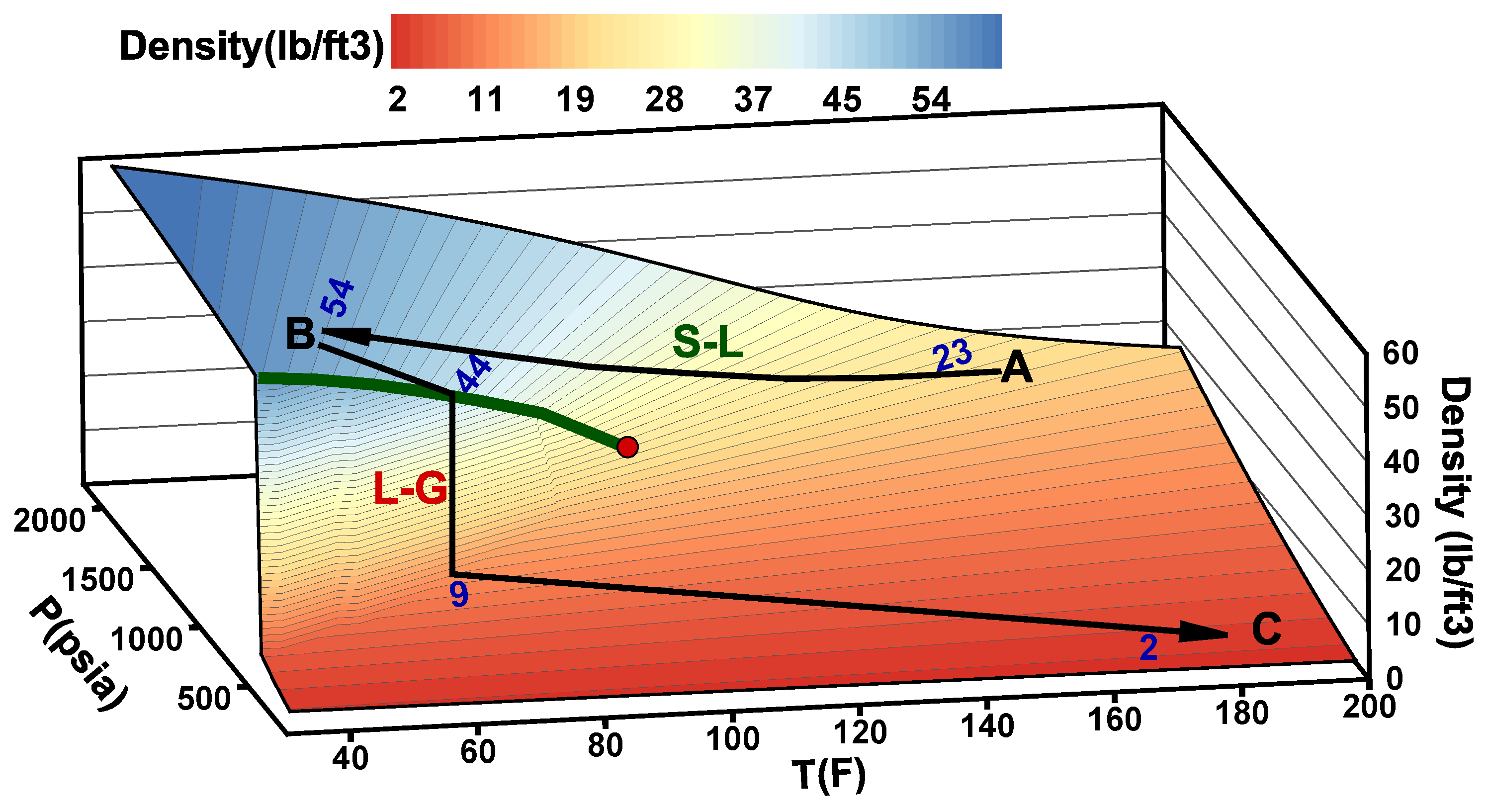
Figure 2 highlights two phase transitions for CO that are expected to occur early in the sequestration process. The first one corresponds to the supercritical-to-liquid (S–L) phase transition that occurs within the pipeline that connects the onshore CO source with the offshore surface wellhead. The second one corresponds to the L–G phase transition that occurs somewhere between the wellhead and the reservoir, as discussed above. While the S–L phase transition is gradual and smooth in terms of the change in CO properties, the L–G phase transition is abrupt and discontinuous. The CO density behavior is presented in Figure 3, which shows the smooth density behavior of CO during the S–L phase transition (AB line) and the discontinuity at the liquid–gas interface during the L–G phase transition (BC line). The density drops by a factor of about five.
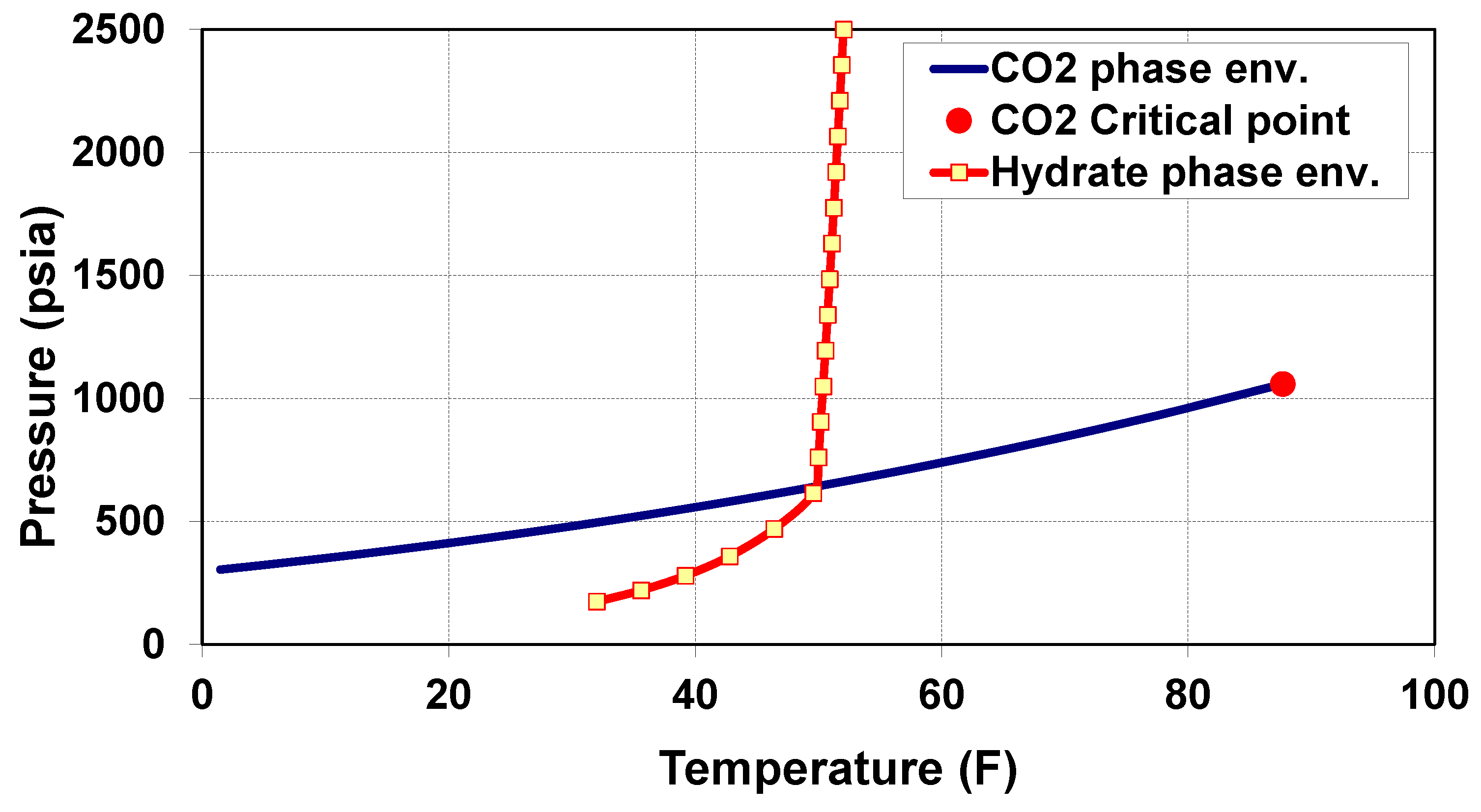
A CO-water mixture under certain PVT conditions will form a solid hydrate phase that looks like ice. The hydrate-formation (HF) temperature (HFT) is, however, much higher than that of ice or dry ice. Consequently, if CO is not fully dehydrated and water is present, then CO hydrates are likely to form before ice forms. The hydrate-formation envelope for a CO-water system and the CO PT diagram are shown in Figure 4. The hydrate-formation temperature is around 53 F (10 C). If water and CO coexist within the PT region on the left side of the hydrate phase envelope, then CO hydrates will form. Minerals, such as NaCl or KCl, act as natural hydrate inhibitors that can reduce HF. For instance, 2 wt.% of NaCl reduces HFT to 43 F (6 C). The CO phase envelopes and the hydrate HFT plots are based on multiphase flash calculations [42,43] generated using the PVTSim software by Calsep.
4. CO Thermodynamic Phase Behavior in the Wellbore
Early during the injection process, while the pressure in the reservoir builds up to the CO bubble point, the injected CO will vaporize. The CO flash point will be reached at a location between the wellhead and the subsurface reservoir, leading to the following possible scenarios:
- Scenario 1—CO vaporization within the well tubing: If CO vaporizes within the well tubing and is not completely dry (i.e., water is present), then hydrates may form within the tubing [27]. On the other hand, if water is absent, as expected, no hydrates will form inside the tubing. However, the risk of hydrate formation due to vaporization within the well tubing will remain relevant within the reservoir as the cooled gaseous CO hits wet sand near the wellbore.
- Scenario 2—CO vaporization across the perforations: CO vaporization across the well perforations or within 1–2 feet of the wellbore could be the worst scenario. Cooling would be more localized, possibly causing hydrates or even dry ice to form across the perforations, resulting in a loss of injectivity.
- Scenario 3—CO vaporization within the reservoir: CO vaporization within the reservoir formation, away from the wellbore, is less problematic since hydrate formation is unlikely to result in complete plugging. Nevertheless, this scenario may cause partial loss of injectivity.
The location at which CO reaches its flash point is expected to vary in time as a function of the injection rate, the tubing head pressure (THP), and the bottom-hole pressure (BHP). To further analyze the flow behavior of CO within the well tubing, we used two modeling approaches. The first one is a commonly used decoupled approach that models the flow performance of steady-state CO in the wellbore. With the decoupled approach, the flow in the wellbore is analyzed at the steady state without accounting for the transient response of the reservoir. We introduce a coupled approach that integrates the transient flow both within the wellbore and in the reservoir. The limitation of the decoupled approach is that it misses the liquid-to-gas transition state of CO, which results in a pressure gap at the wellhead. In contrast, the coupled approach captures the liquid-to-gas transition stage and therefore resolves the pressure gap issue, as will be detailed later. The geothermal gradient, including the subsea temperature and thermal conductivity, between the fluid in the wellbore and the surrounding environment are considered. In the following sections, we discuss the results from both the decoupled and the coupled approaches.
5. Decoupled Approach
With this approach, we study the behavior of steady-state CO in the wellbore under static and dynamic conditions (i.e., during CO injection).
5.1. Behavior under Static Conditions
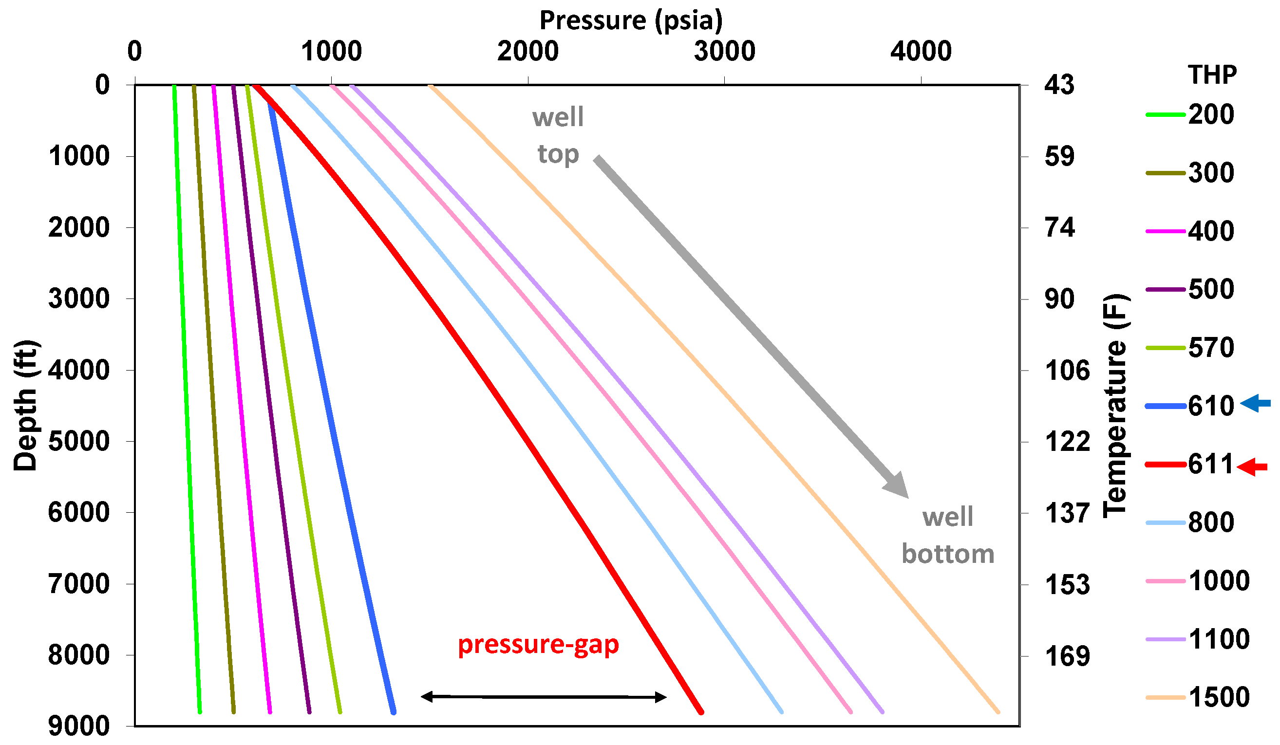
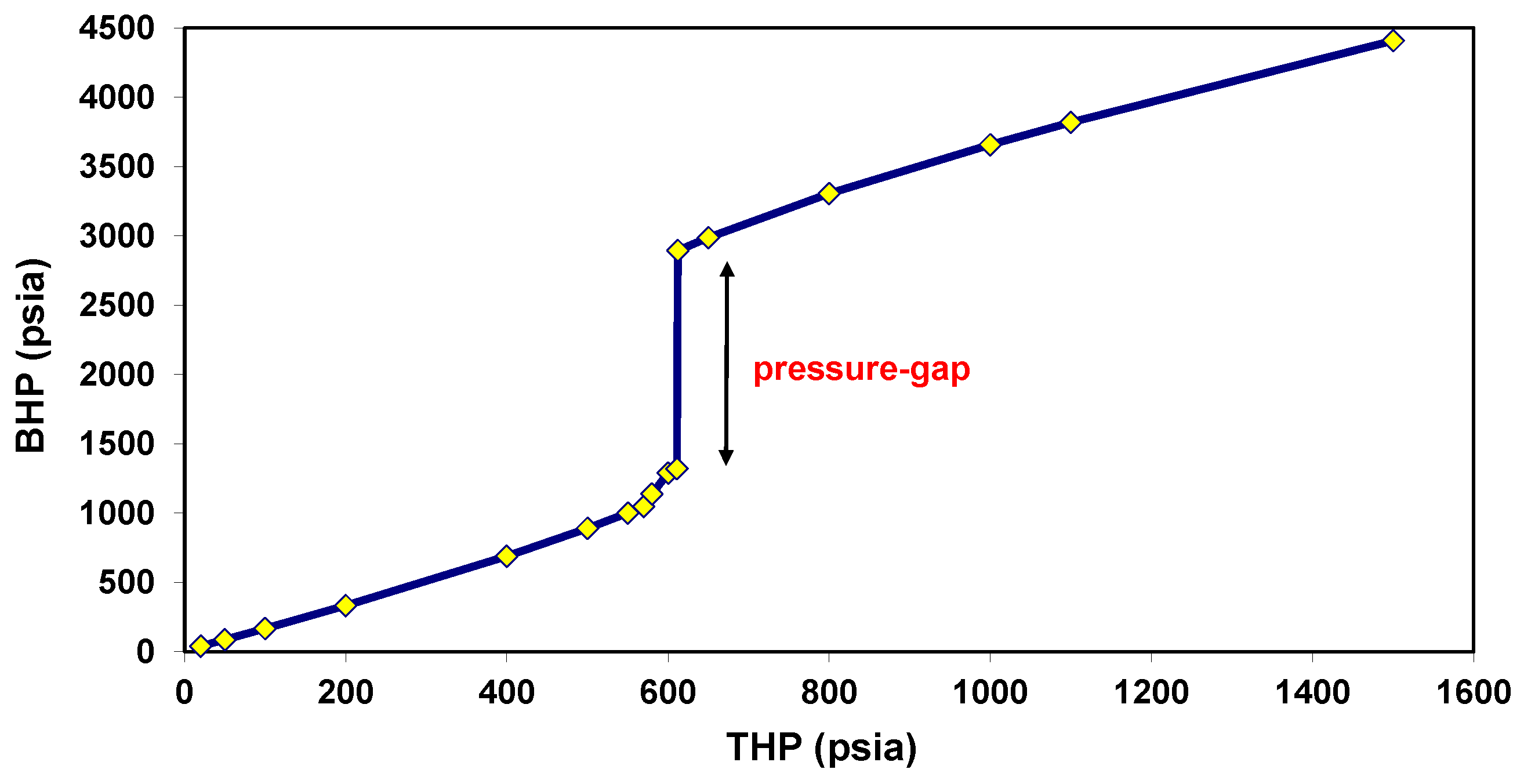
We investigate the CO phase behavior and bottom-hole pressure (BHP) in the wellbore under hydrostatic conditions (non-flowing) with different operational conditions for a range of THP scenarios. The relevant data for this model is provided in Table 1. Hydrostatic conditions may occur during shut-in times, when the pressure in the wellbore reaches equilibrium with the reservoir pressure, and the fluid temperature corresponds to the natural geothermal gradient. Here, we consider the case of CO in the liquid state at 43 F. Density and phase behavior calculations for CO were performed using the Peng–Robinson EOS [44]. Table 2 provides the relevant input parameters. Under static conditions, friction is irrelevant; therefore, the pressure profile in the well column is independent of the tubing diameter. Figure 5 shows the CO pressure in the wellbore versus depth and versus temperature for the different THP scenarios. When THP is gradually increased from THP = 610 psia to THP = 611 psia, a discontinuous behavior (i.e., a pressure gap) appears in the BHP.
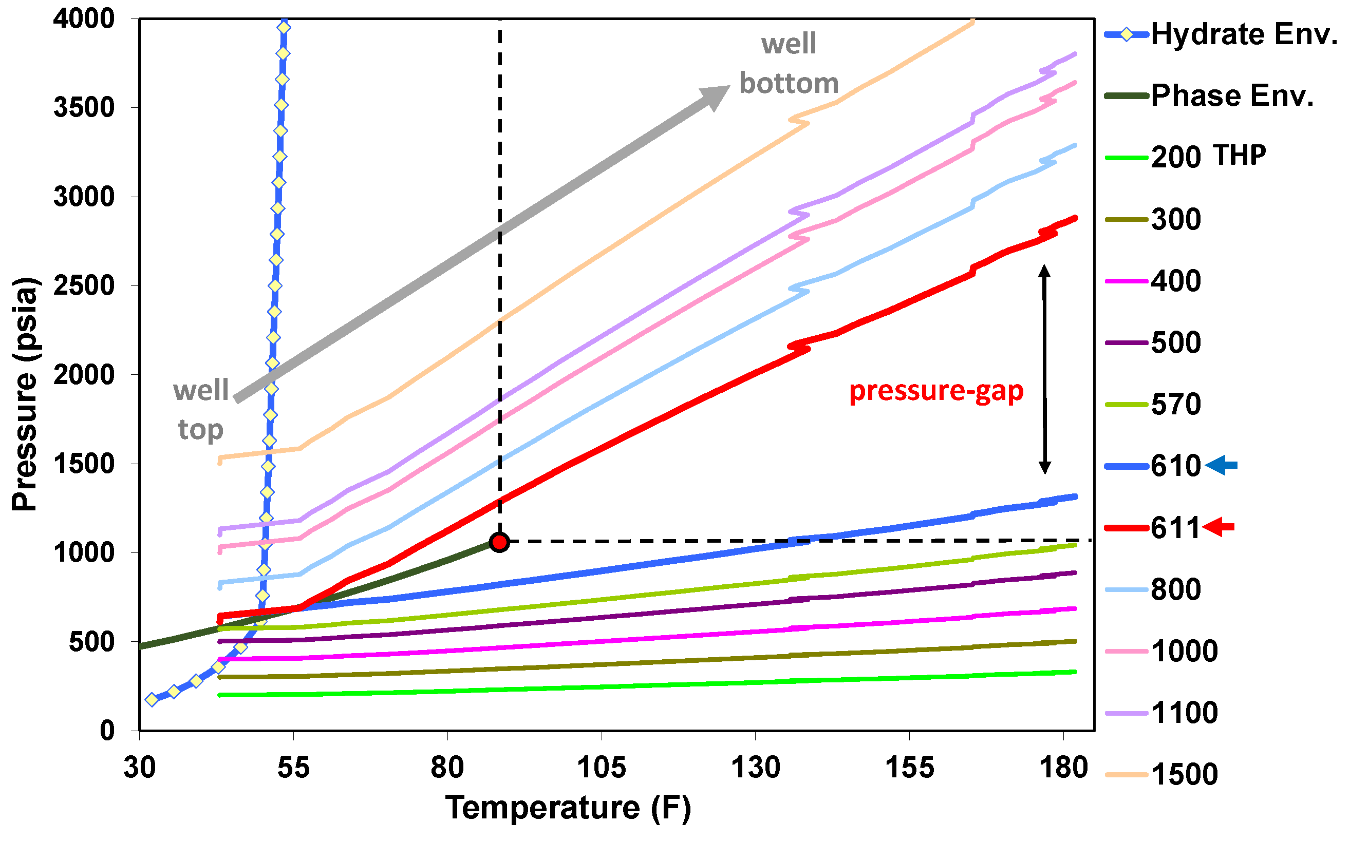
In Figure 6, we superimpose the PT curves shown in Figure 5 on the CO PT phase envelope. This plot shows the PT conditions where CO would be in the supercritical, liquid, and gas states within the wellbore. For any THP scenario below 610 psia, which is around the CO bubble-point pressure at T = 43 F, CO will be in the gas state throughout most of the wellbore. With a slight increase in THP (611 psia), CO converts to a dense state (liquid or supercritical), and a jump in BHP occurs. In Figure 7, we plot BHP versus THP, the values of which were obtained from the pressure profiles shown in Figure 5, to highlight the pressure gap observation. This pressure gap, which is a result of the discontinuity between the liquid CO and gaseous CO densities, may wrongly imply that THP cannot be controlled well enough to achieve a smooth behavior in BHP.
5.2. Behavior under Dynamic Conditions
We performed similar calculations to assess the pressure behavior within the wellbore under dynamic conditions, i.e., during CO injection. We note that THP represents the injection pressure, which can be controlled at the wellhead to achieve the desired injection rate. The pressure and temperature profiles under dynamic conditions vary as a function of the pressure loss due to friction in the tubing and temperature changes due to heat exchange (loss or gain) with the medium surrounding the wellbore. To address the impact of the injection rate and temperature, we consider four test cases where we vary the injection rate (R) and the surface temperature of the injected during CO injection (T) as follows:

| Case | Injection Rate (MMSCF/day) * | (F) |
| 1 | 15 | 43 |
| 2 | 15 | 100 |
| 3 | 50 | 43 |
| 4 | 50 | 100 |
* MMSCF/day: million cubic feet per day at standard conditions.
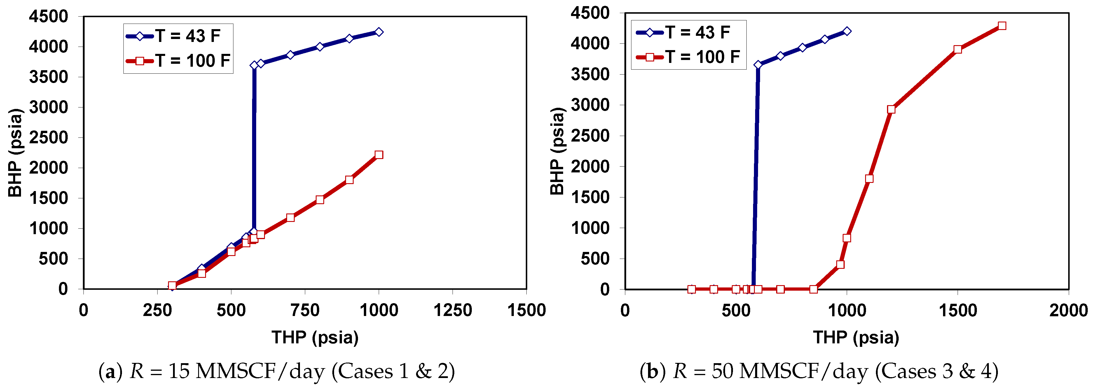
We emphasize that at a low temperature (T = 43 F), CO is in the liquid state, and therefore, a liquid-to-gas transition will occur; at a high temperature (T = 100 F), CO is in the supercritical state, and therefore, a supercritical-to-gas transition will occur. Figure 8a,b show the BHP versus THP plots under dynamic conditions for Cases 1–2 and 3–4, respectively. A pressure gap appears in the BHP profile for the cases with a low temperature (Cases 1 and 3), similar to our results under static conditions (Figure 7). On the other hand, the BHP–THP curve is continuous at a high temperature, i.e., when CO is injected in the supercritical state (Cases 2 and 4). We note that the BHP–THP relationship at a given injection rate (R) influences the surface injection pressure (i.e., THP) that is required to maintain the desired injectivity as the reservoir pressure (i.e., BHP) builds up. When BHP appears to be zero in Figure 8b (Case 4), this is an indication that the desired injection rate cannot be achieved at a particular THP; therefore, a higher THP is required. Unfortunately, this decoupled approach, though commonly used in the literature, does not provide an adequate representation of the pressure or injectivity behaviors. Therefore, an alternative model is needed.
6. Coupled Approach
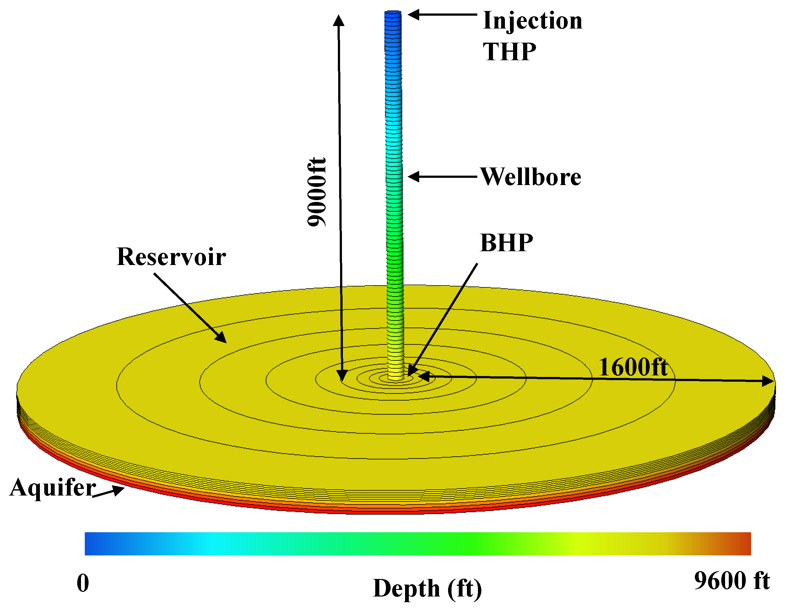
Integrated wellbore and reservoir models were built using a compositional reservoir simulator, Eclipse by Schlumberger. Our objective is to study the CO flow behavior in the wellbore under transient conditions and to investigate the BHP–THP relationship with emphasis on the pressure gap issue in particular. One common method of coupling the fluid flow in the reservoir and the wellbore is to use vertical lift performance (VLP) curves, which can be provided as lookup tables in the reservoir simulator. VLP tables describe the relationship between BHP and THP at different injection rates. As the VLP curves are expected to be continuous and monotonic, the discontinuity in BHP makes this approach unfeasible. Imposing artificial smoothing on the discontinuities would produce wrong results. To overcome this challenge, we build a simulation model that explicitly incorporates both the wellbore and the reservoir. We use a 3D radial model that mimics the reservoir, including the aquifer, the reservoir, and the overburden. The innermost radial grid blocks are used to represent the wellbore, and the outer grid blocks represent the aquifer, the reservoir, and the reservoir overburden, as shown in Figure 9. The model properties are provided in Table 2 and Table 3.
The grid blocks representing the wellbore are assigned a porosity of 100% and a permeability of 10,000 Darcy. The permeability was tuned to mimic the pressure drop, including the friction effect, within the wellbore. The top wellbore grid block is set as the injection point (see Figure 9). The well THP is controlled to achieve a constant injection rate. The injection pressure at the wellhead represents THP, and the pressure at the top perforation in the reservoir represents BHP (see Figure 9). The model satisfactorily captures the impact of temperature variation with depth on the CO thermodynamic properties and phase behavior. Here, we consider two cases. In the first case, we assume that CO is injected in its supercritical state at T = 100 F. In the second case, we assume that CO is injected in its liquid state at T = 60 F. The two cases are detailed below.
6.1. Case 1: Injection of CO in the Supercritical State
In this case, we assume that CO is injected in its supercritical state at 100 F with a target injection rate of 50 MMSCF/day. As discussed previously, injecting CO at a high temperature (i.e., under supercritical conditions) at the wellhead will result in a supercritical-to-gas transition, which is a smooth and continuous phase transition. The well injectvity is controlled by the rate of injection, and therefore, the model will determine the minimum THP needed to inject at the desired rate. The calculated BHP is a result of THP, the injection rate, and the reservoir pressure. Pressure and density are recorded in the wellbore at different times. Figure 10a,b show, respectively, the pressure and density profiles in the wellbore as the reservoir pressure builds up over time.
We observe two distinct behaviors in the pressure profiles. At early injection times (<4 years), the pressure decreases with depth as a result of the backpressure provided by the reservoir. At later injection times (>4 years), the pressure increases with depth as the reservoir pressure builds up. The density follows a similar trend. At early injection times, the density exhibits a smooth decreasing trend with depth as CO converts from the supercritical state to the gas state, driven by the low reservoir pressure (Figure 10a). At later times, as the reservoir pressure builds up, CO is in its supercritical state throughout the whole wellbore. The density has a smooth increasing trend with depth, resulting from the higher CO compressibility as pressure increases. The well THP and BHP versus time are shown in Figure 11a. Even as BHP increases by about 2000 psia during the first 20 years of injection, THP increases by less than 100 psia and is able to maintain the desired injection rate. The injection pressure is naturally supported by the increasing weight of CO as it gets denser with pressure. The BHP–THP curves generated by this coupled model and by the previously discussed decoupled model are shown in Figure 11b. They show consistent trends, as expected. We note that the selection of the wellbore permeability is based on the calibration for one point in the BHP–THP curve. The objective here is not to get an exact match between the two models, but rather to better understand their synergy.
6.2. Case 2: Injection of CO in the Liquid State
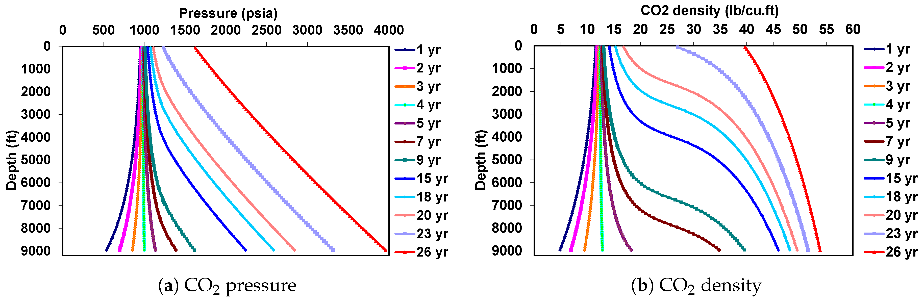
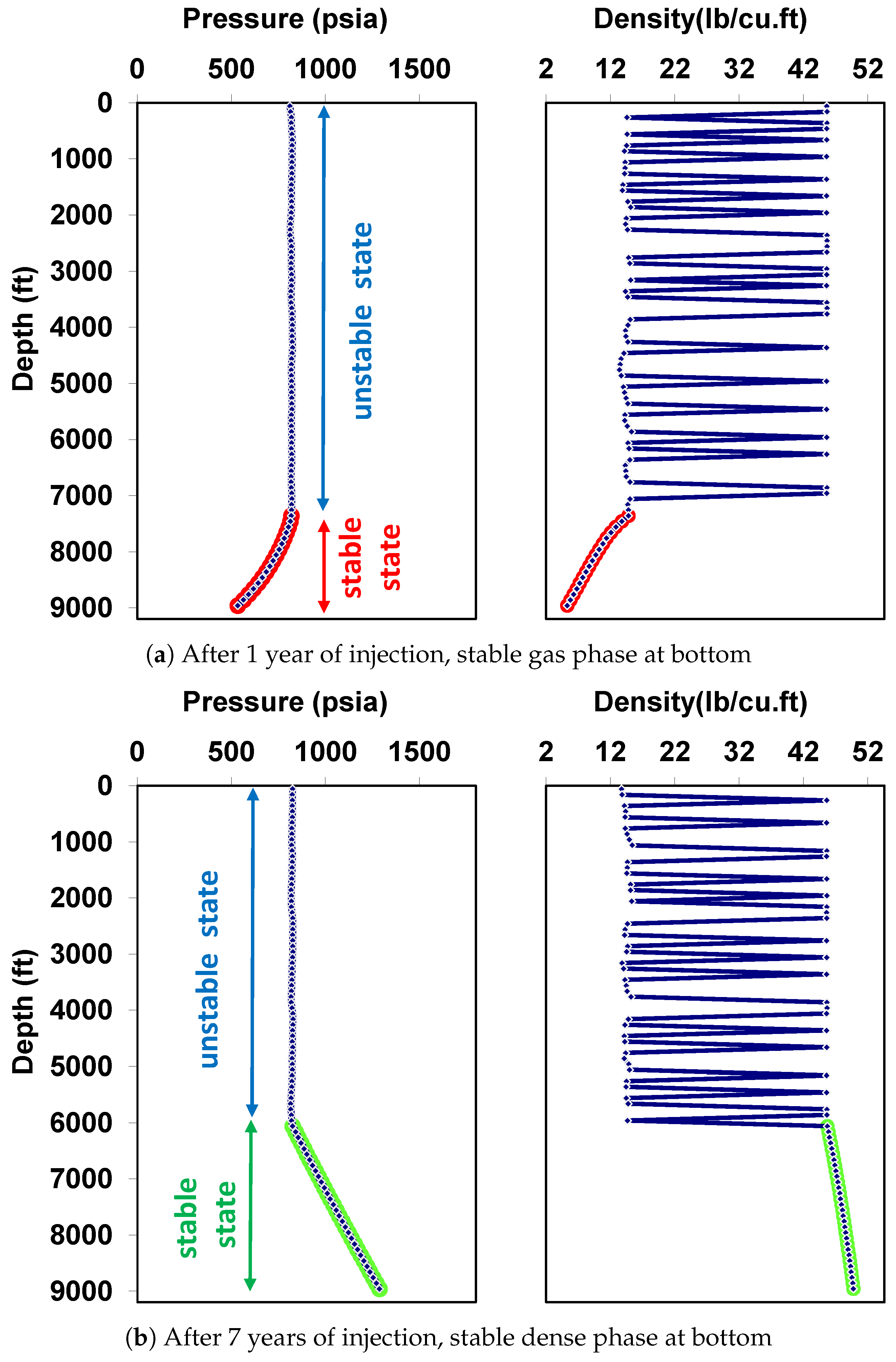
In this case, CO is injected in its liquid state (60 F) with the same target injection rate at the wellhead as in the previous case, i.e., 50 MMSCF/day. The current case, however, is more challenging as discontinuities in the CO properties will occur as CO transitions from a liquid to a gas. Figure 12a shows the pressure profile and the density of CO versus depth after a year of injection. The pressure and density behaviors show two distinct states for CO. A stable CO gas state forms in the lower section of the wellbore (highlighted in red) where the pressure is below the CO bubble-point pressure. In the upper region of the wellbore, CO shows an interesting behavior that corresponds to a thermodynamically unstable state. This unstable state is a two-phase gas–liquid state where CO gas and CO liquid coexist. The pressure in the wellbore is roughly equal to the bubble-point pressure, and the density fluctuates between the gas-phase and liquid-phase densities. Therefore, the upper region is neither gas nor liquid; rather, it is an unstable two-phase state. This behavior cannot be captured using steady-state models.
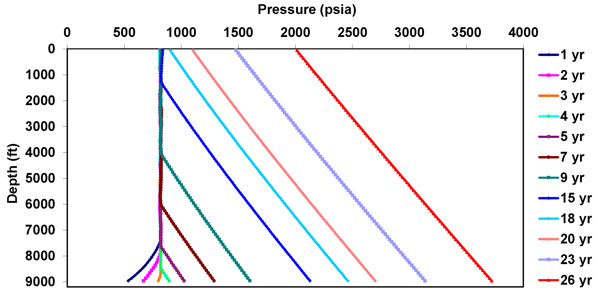
Figure 12b shows the pressure profile and the density of CO versus depth after 7 years of injection. A similar behavior appears. One key difference can be observed in the state behavior of CO in the lower section of the wellbore. As the reservoir pressure builds up, the pressure in the lower section exceeds the CO bubble-point pressure. Thus, the CO gas converts to a stable dense phase. CO in the upper region is still in an unstable two-phase state. To draw a complete picture, Figure 13 shows the pressures at different times during the injection period, versus depth.
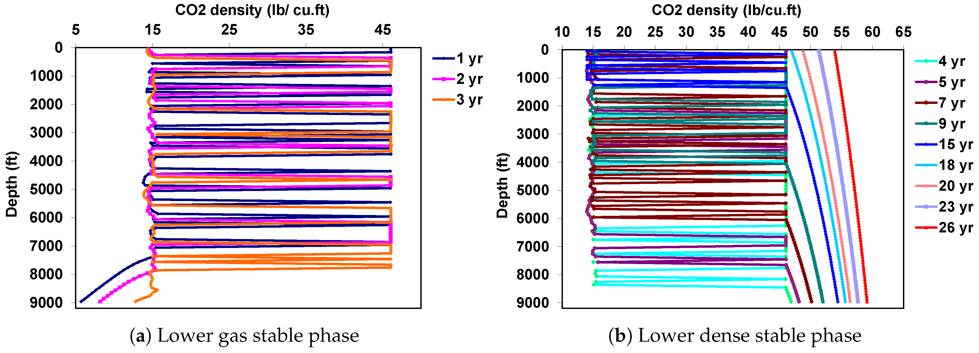
The unstable two-phase region disappears after 18 years of injection as the pressure throughout the entire wellbore exceeds the CO bubble-point pressure. The corresponding densities are plotted in the left panel of Figure 14, which shows a stable gas region and an unstable two-phase region. Similarly, the right panel in Figure 14 shows a stable dense-phase region and an unstable two-phase region co-occurring in the wellbore up until 18 years of injection. After 18 years, CO is in a stable dense state throughout the entire wellbore.
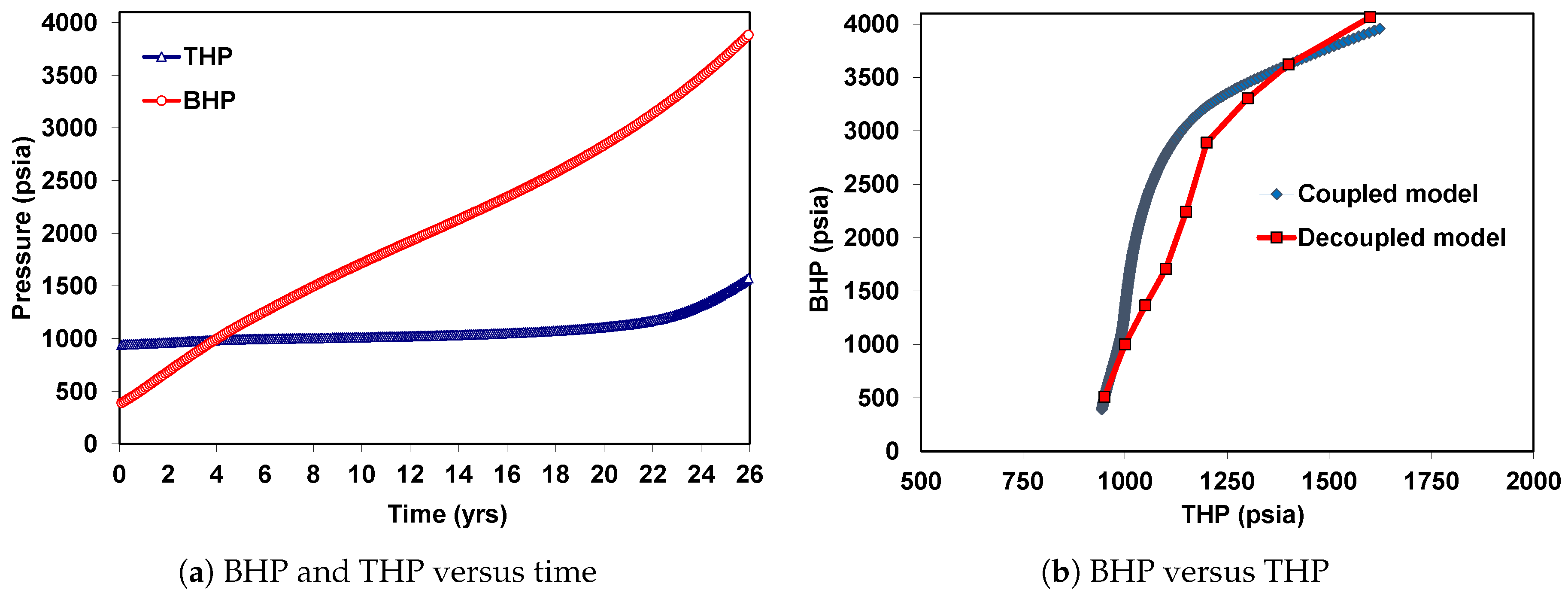
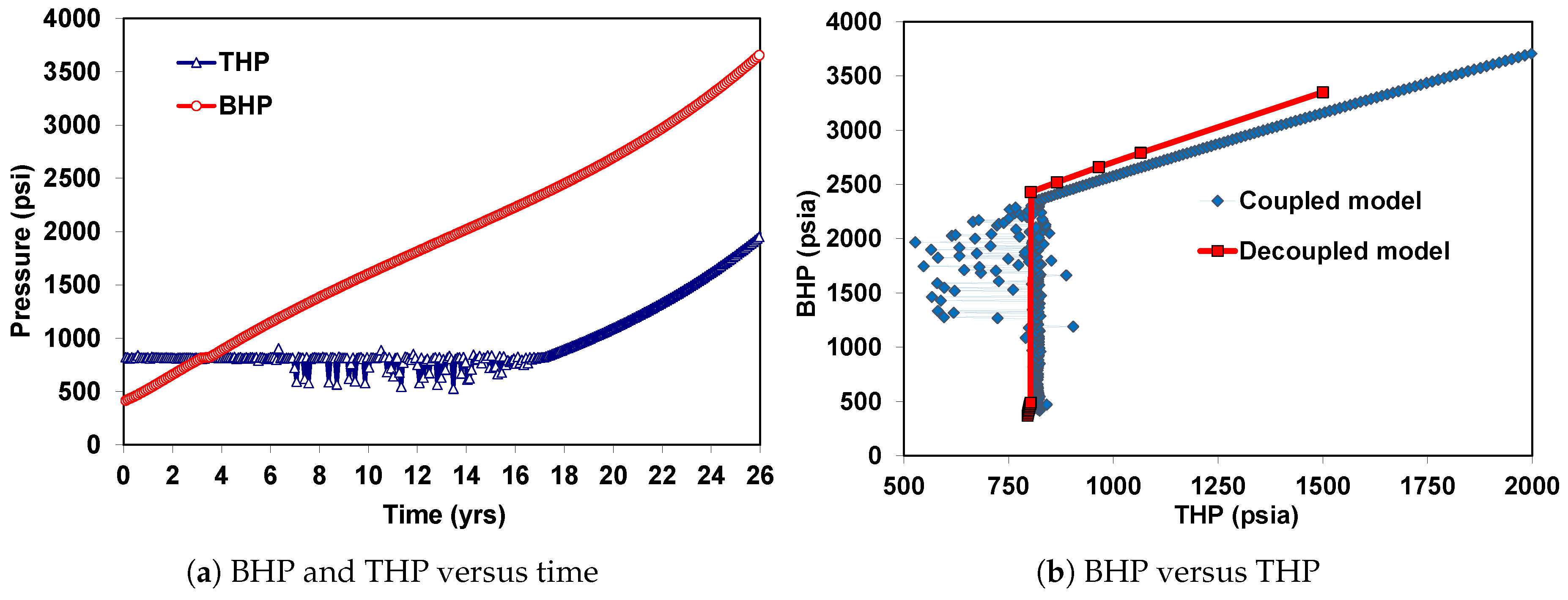
The well BHP and THP are shown as functions of time in Figure 15a. Until 18 years of injection, the wellhead pressure remains roughly constant, and a constant injection rate is maintained, whereas BHP increases as CO fills up the reservoir. THP starts to increase when CO is in the dense phase throughout the entire wellbore because no more injectivity support comes from gravity (i.e., CO weight in the column). The BHP–THP curve from this coupled model is shown in Figure 15b and compared to the BHP–THP curve obtained from the decoupled model. The two approaches appear to be consistent. However, a key difference is the BHP jump (i.e., pressure gap) produced by the decoupled model, which is unrealistic. This limitation of the decoupled model is related to the steady-state assumption, where the unstable two-phase CO in the upper region of the wellbore cannot be captured.
7. CO Heating
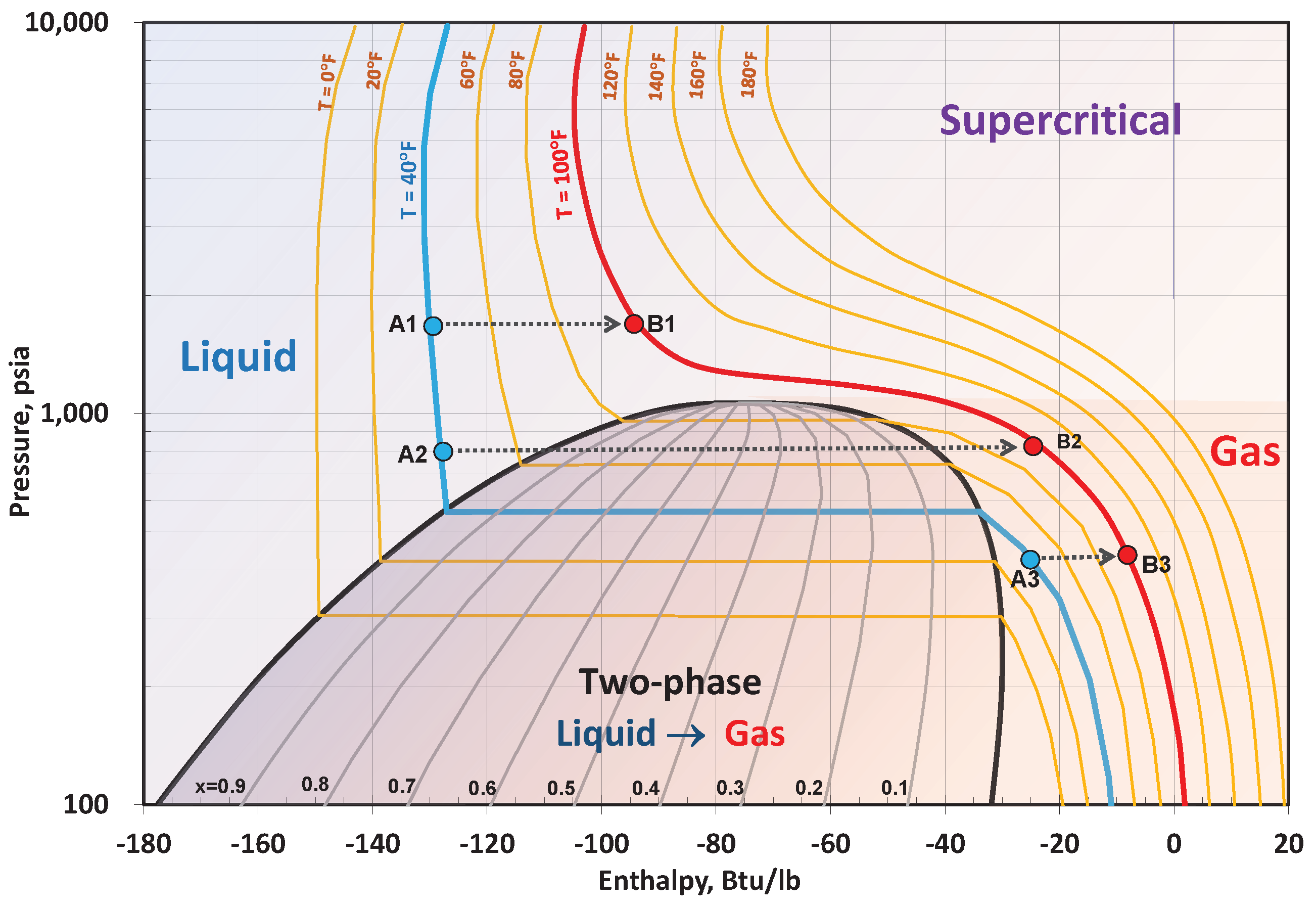
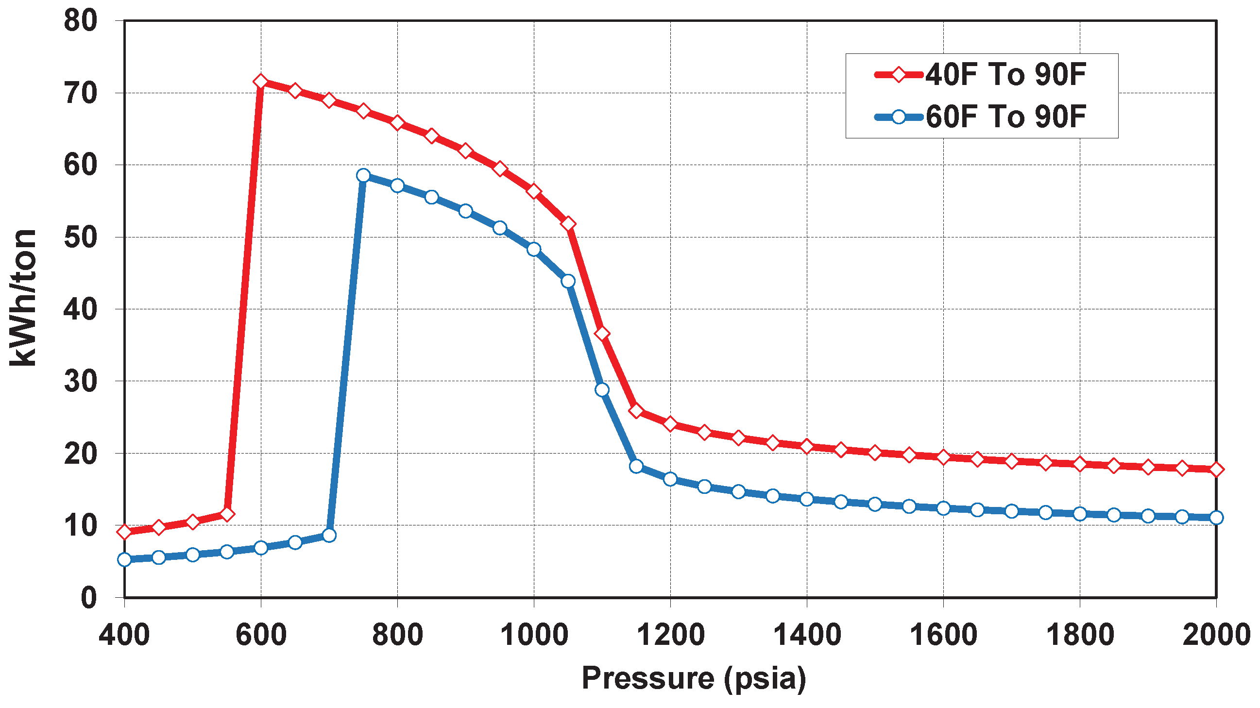
As discussed previously, injecting CO in its liquid state could be an operational hazard. One potential remedy to overcome this issue is to heat CO at the wellhead. Then, CO will be injected in its supercritical state. There are other potential solutions, such as the use of hydrate inhibitors, but they are not discussed in this work. In this section, we provide a rough estimate of the energy required to convert CO from the liquid to the supercritical state by heating. The required energy depends on the initial and the final temperature of CO. Here, we assess two scenarios: (1) heating CO from 40 F to 90 F, and (2) heating CO from 60F to 90F. The energy required to heat CO can be roughly calculated from the pressure–enthalpy diagram shown in Figure 16. CO enthalpies during the initial and final stages are from the NIST chemistry webbook (NIST, 2011). The required energy is a function of the initial pressure, the final pressure, and the temperature. For instance, to heat CO by 60F (e.g., from T = 40 F to T = 100 F) at a constant pressure of 1000 psia, the required enthalpy difference is about 100 Btu/lb (see Figure 16), which corresponds to roughly 65 kWh per metric ton of CO (1 Btu = 0.000293 kWh; 1 ton = 2204.6 lb). The required enthalpy depends strongly on the initial state of CO. Consider the three scenarios, A1, A2, and A3, shown in Figure 16. The most energy-demanding scenario to heat A1-to-B1 (liquid-to-liquid), A2-to-B2 (liquid-to-gas), and A3-to-B3 (gas-to-gas) corresponds to the condition that involves phase transition (i.e., latent heat). Figure 17 shows the energy requirements for the two scenarios (40 F to 90 F and 60 F to 90F) as a function of pressure. As the injection pressure is expected to be within the range of 600–1000 psia, the energy required to convert CO from the liquid to the supercritical state is roughly 60–70 kWh per metric ton of CO.
8. Conclusions
This work addressed an operational challenge related to the injectivity of CO in depleted gas reservoirs. Injecting CO in its dense state into a low-pressure reservoir will result in CO vaporizing within either the wellbore or the subsurface reservoir formation. The vaporization process is associated with a temperature drop because of the Joule–Thomson effect, abrupt variations in the thermodynamic properties of the CO phases, and an increased flow velocity because of CO expansion. These phenomena could be hazardous as they may cause flow assurance issues such as the formation of hydrates, loss of pressure control, and compromised integrity of the wellbore. Understanding the flow behavior of CO in the wellbore was the main focus of this work. We showed that the commonly used decoupled modeling approach is not adequate to describe the flow behavior of CO when a liquid-to-gas transition occurs inside the wellbore. The decoupled approach predicts a discontinuity in the bottom-hole pressure (i.e., a pressure gap), which is unrealistic. The inherent limitation of the decoupled approach is its inability to capture the transient effect that occurs during the CO vaporization process. We proposed an alternative, coupled approach that integrates the flow in both the wellbore and the reservoir. This new approach explained the pressure gap issue and showed, for the first time, that the liquid-to-gas transition of CO is not instantaneous and not localized. The model showed two distinct behaviors of CO in two regions of the wellbore. CO in the lower region of the wellbore was in a stable single-phase state, and CO in the upper region was in an unstable two-phase state. Within the two-phase region, liquid and gas CO coexist. This behavior enabled a gradual and continuous build-up in the bottom-hole pressure, which was not captured correctly by the decoupled approach. We also evaluated one possible solution to the liquid-to-gas transition issue, which is to convert CO from the liquid to the supercritical state by increasing its temperature at the wellhead. We estimated that 60 to 70 kWh per metric ton of CO would be required to sufficiently increase the temperature of CO. There could be additional costs depending on the efficiency of the facility and the heat exchanges.
Author Contributions
The three authors, H.H., M.F., and M.R.S. discussed the importance of the topic and formalized the key idea. H.H. conducted the simulations. The three authors interpreted the results and contributed to the manuscript editing.
Funding
This research received no external funding.
Acknowledgments
The first author would like to thank Schlumberger Ltd. for granting KAUST academic licenses for Eclipse, and would like also to thank Calsep for providing an academic license for PVTsim Nova.
Conflicts of Interest
The authors declare no conflicts of interest.
References
- Stocker, T. Climate Change 2013: The Physical Science Basis: Working Group I Contribution to the Fifth Assessment Report of the Intergovernmental Panel on Climate Change; Cambridge University Press: Cambridge, UK, 2014; p. 1535. [Google Scholar]
- Rose, S.K.; Richels, R.; Blanford, G.; Rutherford, T. The Paris Agreement and next steps in limiting global warming. Clim. Chang. 2017, 142, 255–270. [Google Scholar] [CrossRef]
- Cook, J.; Oreskes, N.; Doran, P.T.; Anderegg, W.R.L.; Verheggen, B.; Maibach, E.W.; Carlton, J.S.; Lewandowsky, S.; Skuce, A.G.; Green, S.A.; et al. Consensus on consensus: A synthesis of consensus estimates on human-caused global warming. Environ. Res. Lett. 2016, 11, 048002. [Google Scholar] [CrossRef]
- Verheggen, B.; Strengers, B.; Cook, J.; van Dorland, R.; Vringer, K.; Peters, J.; Visser, H.; Meyer, L. Scientists’ Views about Attribution of Global Warming. Environ. Sci. Technol. 2014, 48, 8963–8971. [Google Scholar] [CrossRef] [PubMed]
- Sharma, S.S. Determinants of carbon dioxide emissions: Empirical evidence from 69 countries. Appl. Energy 2011, 88, 376–382. [Google Scholar] [CrossRef]
- Pachauri, R.K.; Allen, M.R.; Barros, V.R.; Broome, J.; Cramer, W.; Christ, R.; Church, J.A.; Clarke, L.; Dahe, Q.; Dasgupta, P.; et al. Climate Change 2014: Mitigation of Climate Change: Working Group III Contribution to the Fifth Assessment Report of the Intergovernmental Panel on Climate Change; Cambridge University Press: New York, NY, USA, 2015. [Google Scholar]
- IEA. 20 Years of Carbon Capture and Storage Accelerating Future Deployment; IEA: Paris, France, 2016. [Google Scholar] [CrossRef]
- Godec, M.; Kuuskraa, V.; Van Leeuwen, T.; Melzer, L.S.; Wildgust, N. CO2 Storage in Depleted Oil Fields: The Worldwide Potential for Carbon Dioxide Enhanced Oil Recovery. Energy Procedia 2011, 4, 2162–2169. [Google Scholar] [CrossRef]
- Bruhn, T.; Naims, H.; Olfe-Kräutlein, B. Separating the debate on CO2 utilisation from carbon capture and storage. Environ. Sci. Policy 2016, 60, 38–43. [Google Scholar] [CrossRef]
- Rogelj, J.; den Elzen, M.; Hohne, N.; Fransen, T.; Fekete, H.; Winkler, H.; Chaeffer, R.S.; Ha, F.; Riahi, K.; Meinshausen, M. Paris Agreement climate proposals need a boost to keep warming well below 2 degrees C. Nature 2016, 534, 631–639. [Google Scholar]
- Ladbrook, B.; Smith, N.; Pershad, H.; Harland, K.; Slater, S.; Holloway, S.; Kirk, K. CO2 Storage in Depleted Gas Fields. IEA Technical Report. 2009. Available online: https://hub.globalccsinstitute.com/sites/default/files/publications/95786/co2-storage-depleted-gas-fields.pdf (accessed on 24 April 2019).
- Koide, H.; Tazaki, Y.; Noguchi, Y.; Iijima, M.; Ito, K.; Shindo, Y. Underground-Storage of Carbon-Dioxide in Depleted Natural-Gas Reservoirs and in Useless Aquifers. Eng. Geol. 1993, 34, 175–179. [Google Scholar] [CrossRef]
- Winter, E.M.; Bergman, P.D. Availability of Depleted Oil and Gas-Reservoirs for Disposal of Carbon-Dioxide in the United-States. Energy Convers. Manag. 1993, 34, 1177–1187. [Google Scholar] [CrossRef]
- Gunter, W.; Wong, S.; Cheel, D.; Sjostrom, G. Large CO2 Sinks: Their role in the mitigation of greenhouse gases from an international, national (Canadian) and provincial (Alberta) perspective. Appl. Energy 1998, 61, 209–227. [Google Scholar] [CrossRef]
- Seo, J.G.; Mamora, D.D. Experimental and Simulation Studies of Sequestration of Supercritical Carbon Dioxide in Depleted Gas Reservoirs. In Proceedings of the Exploration and Production Environmental Conference, San Antonio, TX, USA, 10–12 March 2003. [Google Scholar] [CrossRef]
- Oldenburg, C.M.; Benson, S.M. CO2 Injection for Enhanced Gas Production and Carbon Sequestration. In Proceedings of the SPE International Petroleum Conference and Exhibition in Mexico, Villahermosa, Mexico, 10–12 February 2002. [Google Scholar] [CrossRef]
- Clemens, T.; Wit, K. CO2 Enhanced Gas Recovery Studied for an Example Gas Reservoir. In Proceedings of the SPE Annual Technical Conference and Exhibition, San Antonio, TX, USA, 29 September–2 October 2002. [Google Scholar] [CrossRef]
- Holloway, S.; Vanderstraaten, R. The Joule-Ii Project the Underground Disposal of Carbon-Dioxide. Energy Convers. Manag. 1995, 36, 519–522. [Google Scholar] [CrossRef]
- Holloway, S. An overview of the Joule II project the underground disposal of carbon dioxide. Energy Convers. Manag. 1996, 37, 1149–1154. [Google Scholar] [CrossRef]
- Li, Z.W.; Dong, M.Z.; Li, S.L.; Huang, S. CO2 sequestration in depleted oil and gas reservoirs—Caprock characterization and storage capacity. Energy Convers. Manag. 2006, 47, 1372–1382. [Google Scholar] [CrossRef]
- Naylor, M.; Wilkinson, M.; Haszeldine, R.S. Calculation of CO2 column heights in depleted gas fields from known pre-production gas column heights. Mar. Pet. Geol. 2011, 28, 1083–1093. [Google Scholar] [CrossRef]
- Field, C.B.; Barros, V.R.; Intergovernmental Panel on Climate Change. Climate Change 2014 Impacts Adaptation, and Vulnerability: Working Group II Contribution to the Fifth Assessment Report of The Intergovernmental Panel on Climate Change; Cambridge University Press: New York, NY, USA, 2015. [Google Scholar]
- Jiang, X. A review of physical modelling and numerical simulation of long-term geological storage of CO2. Appl. Energy 2011, 88, 3557–3566. [Google Scholar] [CrossRef]
- Welkenhuysen, K.; Rupert, J.; Compernolle, T.; Ramirez, A.; Swennen, R.; Piessens, K. Considering economic and geological uncertainty in the simulation of realistic investment decisions for CO2-EOR projects in the North Sea. Appl. Energy 2017, 185, 745–761. [Google Scholar] [CrossRef]
- Espinoza, D.N.; Santamarina, J.C. CO2 breakthrough-Caprock sealing efficiency and integrity for carbon geological storage. Int. J. Greenhouse Gas Control 2017, 66, 218–229. [Google Scholar] [CrossRef]
- Dai, Z.; Zhang, Y.; Bielicki, J.; Amooie, M.A.; Zhang, M.; Yang, C.; Zou, Y.; Ampomah, W.; Xiao, T.; Jia, W.; et al. Heterogeneity-assisted carbon dioxide storage in marine sediments. Appl. Energy 2018, 225, 876–883. [Google Scholar] [CrossRef]
- Maloney, D.R.; Briceno, M. Experimental Investigation of Cooling Effects Resulting from Injecting High Pressure Liquid or Supercritical CO2 into a Low Pressure Gas Reservoir. Petrophysics 2009, 50, 335–344. [Google Scholar]
- Hoteit, H. Modeling the Injectivity-Gap Problem in the Wellbore during CO2 Injection into Low Pressure Reservoirs. In Mathematical & Computational Issues in the Geosciences; SIAM: Long Beach, CA, USA, 2011. [Google Scholar]
- Shell. Storage Development Plan. 2015. Available online: https://assets.publishing.service.gov.uk/government/uploads/system/uploads/attachment_data/file/531016/DECC_Ready_-_KKD_11.128_Storage_Development_Plan.pdf (accessed on 24 April 2019).
- Klotz, I.M.; Rosenberg, R.M. Chemical Thermodynamics: Basic Theory and Methods, 5th ed.; Wiley: New York, NY, USA, 1994. [Google Scholar]
- Tabor, D. Gases, Liquids and Solids: And Other States of Matter, 3rd ed.; Cambridge University Press: Cambridge, UK, 1991. [Google Scholar]
- Jenkins, C.R.; Cook, P.J.; Ennis-King, J.; Undershultz, J.; Boreham, C.; Dance, T.; de Caritat, P.; Etheridge, D.M.; Freifeld, B.M.; Hortle, A.; et al. Safe storage and effective monitoring of CO2 in depleted gas fields. Proc. Natl. Acad. Sci. USA 2012, 109, E35–E41. [Google Scholar] [CrossRef]
- Porse, S.L.; Wade, S.; Hovorka, S.D. Can we Treat CO2 Well Blowouts like Routine Plumbing Problems? A Study of the Incidence, Impact, and Perception of Loss of Well Control. Energy Procedia 2014, 63, 7149–7161. [Google Scholar] [CrossRef]
- Skinner, L. CO2 Blowouts: An Emerging Problem. World Oil 2003, 1, 224. [Google Scholar]
- Xu, Q.J.; Weir, G.F.; Paterson, L.; Black, I.; Sharma, S. A CO2-Rich Gas Well Test and Analyses. In Proceedings of the Asia Pacific Oil and Gas Conference and Exhibition, Jakarta, Indonesia, 30 October–1 November 2007. [Google Scholar] [CrossRef]
- Oldenburg, C.M. Joule-Thomson cooling due to CO2 injection into natural gas reservoirs. Energy Convers. Manag. 2007, 48, 1808–1815. [Google Scholar] [CrossRef]
- Mathias, S.A.; Gluyas, J.G.; Oldenburg, C.M.; Tsang, C.F. Analytical solution for Joule-Thomson cooling during CO2 geo-sequestration in depleted oil and gas reservoirs. Int. J. Greenhouse Gas Control 2010, 4, 806–810. [Google Scholar] [CrossRef]
- Ziabakhsh-Ganji, Z.; Kooi, H. Sensitivity of Joule-Thomson cooling to impure CO2 injection in depleted gas reservoirs. Appl. Energy 2014, 113, 434–451. [Google Scholar] [CrossRef]
- Hughes, D.S. Carbon storage in depleted gas fields: Key challenges. Greenhouse Gas Control Technol. 2009, 1, 3007–3014. [Google Scholar] [CrossRef] [Green Version]
- Galic, H.; Cawley, S.J.; Bishop, S.R.; Gas, F.; Todman, S. CO2 Injection Into Depleted Gas Reservoirs. In Proceedings of the Offshore Europe, Aberdeen, UK, 8–11 September 2009. [Google Scholar] [CrossRef]
- Lake, L. Petroleum Engineering Handbook: Indexes and Standards; Society of Petroleum Engineers: Richardson, TX, USA, 2007. [Google Scholar]
- Michelsen, M.L. Calculation of Hydrate Fugacities. Chem. Eng. Sci. 1991, 46, 1192–1193. [Google Scholar] [CrossRef]
- Munck, J.; Skjoldjorgensen, S.; Rasmussen, P. Computations of the Formation of Gas Hydrates. Chem. Eng. Sci. 1988, 43, 2661–2672. [Google Scholar] [CrossRef]
- Firoozabadi, A. Thermodynamics of Hydrocarbon Reservoirs; McGraw-Hill: New York, NY, USA, 1999; p. 355. [Google Scholar]
Figure 1.
Ice formation from Joule–Thomson (JT) cooling on the exterior of the wellhead system of a CO injection well where CO vaporized from the liquid state to the gas state [35].
Figure 1.
Ice formation from Joule–Thomson (JT) cooling on the exterior of the wellhead system of a CO injection well where CO vaporized from the liquid state to the gas state [35].

Figure 2.
Pressure–temperature (PT) phase envelope showing the gas, liquid, and supercritical states of CO as a function of pressure and temperature. Points A, B, C, and D, represent the pressure (P) and temperature (T) conditions of CO during different stages of injection. A is the expected P and T after compression at the capture site, B is the expected P and T at the wellhead, C is the (P,T) conditions in the reservoir at the beginning of CO injection, and D is the final (P,T) conditions after filling up the reservoir with CO. S–L represents the transition point of CO from the supercritical to the liquid state, and L–G is the transition point from the liquid to the gas state.

Figure 3.
CO density (lb/ft) versus temperature and pressure shown on a 3D plot including the CO phase stages A, B, and C and their connecting pathlines.
Figure 3.
CO density (lb/ft) versus temperature and pressure shown on a 3D plot including the CO phase stages A, B, and C and their connecting pathlines.

Figure 4.
CO hydrate phase envelope and CO PT phase diagram shown versus pressure and temperature. If water and CO are present within the PT region on the left side of the hydrate phase envelope, then CO hydrates will form.
Figure 4.
CO hydrate phase envelope and CO PT phase diagram shown versus pressure and temperature. If water and CO are present within the PT region on the left side of the hydrate phase envelope, then CO hydrates will form.

Figure 5.
CO pressure within the wellbore versus depth and versus temperature, drawn from the top to the bottom of the well for different tubing head pressure (THP) scenarios. As CO transitions from liquid to gas, a gap appears in the bottom-hole pressure (BHP).
Figure 5.
CO pressure within the wellbore versus depth and versus temperature, drawn from the top to the bottom of the well for different tubing head pressure (THP) scenarios. As CO transitions from liquid to gas, a gap appears in the bottom-hole pressure (BHP).

Figure 6.
CO pressure and temperature within the wellbore for different THP scenarios and superimposed on the CO phase envelope. The hydrate-formation envelope is also shown for reference. There are PT situations that fall within the hydrate-formation region.
Figure 6.
CO pressure and temperature within the wellbore for different THP scenarios and superimposed on the CO phase envelope. The hydrate-formation envelope is also shown for reference. There are PT situations that fall within the hydrate-formation region.

Figure 7.
BHP versus THP shown under static conditions where a pressure gap appears.

Figure 8.
BHP versus THP plots under dynamic conditions with two cases for CO injection, R = 15 MMSCF/day (left, a) and R = 50 MMSCF/day (right, b) and two cases for the injected CO fluid temperature at the wellhead, T = 43F and T = 100 F. A pressure jump appears in BHP when CO is injected in its liquid state (T = 43 F), whereas BHP is smooth when CO is injected in its supercritical state (T = 100 F).

Figure 9.
Radial model coupling the wellbore, the reservoir, and the aquifer, where the color map shows the depth.
Figure 9.
Radial model coupling the wellbore, the reservoir, and the aquifer, where the color map shows the depth.

Figure 10.
CO behavior in the wellbore vs. depth; Case 1 with CO injected in its supercritical state.
Figure 10.
CO behavior in the wellbore vs. depth; Case 1 with CO injected in its supercritical state.

Figure 11.
BHP and THP versus time from the coupled model (a) and comparison of the BHP–THP curves from the coupled and decoupled models (b).
Figure 11.
BHP and THP versus time from the coupled model (a) and comparison of the BHP–THP curves from the coupled and decoupled models (b).

Figure 12.
Pressure and CO density versus depth in the wellbore after 1 year (a) and 7 years (b) of injection. One unstable two-phase region in the upper section and one stable single phase region in the lower section of the wellbore.
Figure 12.
Pressure and CO density versus depth in the wellbore after 1 year (a) and 7 years (b) of injection. One unstable two-phase region in the upper section and one stable single phase region in the lower section of the wellbore.

Figure 13.
CO pressure in the wellbore vs. depth shown at different times.

Figure 14.
CO density in the wellbore vs. depth at different times; the CO phase-state changes with time as the reservoir pressure builds up. The plot on the left (a) shows one unstable two-phase region and one stable state region. The plot on the right (b) shows one unstable two-phase state and one stable state region until 18 years of injection. As the pressure increases above the bubble-point pressure everywhere in the wellbore (after 18 years), CO forms one stable single-phase phase region throughout the whole wellbore.

Figure 15.
BHP and THP versus time from the coupled model (a) and comparison of the BHP–THP curves from the coupled and decoupled models (b).
Figure 15.
BHP and THP versus time from the coupled model (a) and comparison of the BHP–THP curves from the coupled and decoupled models (b).

Figure 16.
CO pressure–enthalpy diagram showing the CO phase state under different conditions. A1B1, A2B2, and A3B3 lines highlight the enthalpy needed to go from 40 F to 60 F.
Figure 16.
CO pressure–enthalpy diagram showing the CO phase state under different conditions. A1B1, A2B2, and A3B3 lines highlight the enthalpy needed to go from 40 F to 60 F.

Figure 17.
Energy required (kWh/ton) to heat CO versus pressure from two temperature-change scenarios: 40 F to 90 F and 60 F to 90 F.
Figure 17.
Energy required (kWh/ton) to heat CO versus pressure from two temperature-change scenarios: 40 F to 90 F and 60 F to 90 F.

Table 1.
Properties of the well model.
| Well true vertical depth, TVD (ft) | 9000 |
| Well tubing diameter, OD (in) | 5.5 |
| Surface temperature range (F) | 43–60 |
| Reservoir pressure (psia) | 200 |
| Reservoir temperature (F) | 182 |
| Geothermal gradient (F/1000 ft) | 15.7 |
| Injection rate (MMSCF/day) | 15–50 |
Table 2.
Properties of the fluid.
| CO mole fraction | 1 |
| Critical temperature, (F) | 87.7 |
| Critical pressure, (psia) | 1070 |
| Critical volume, (ft/lb-mol) | 1.5 |
| Volume shift, (ft/lb-mol) | −0.1 |
| Acentric factor (–) | 0.24 |
| Molecular weight (g/mol) | 44.01 |
| Parachor (–) | 78 |
Table 3.
Properties of the reservoir model.
| Reservoir depth (ft) | 9000 |
| Reservoir thickness (ft) | 250 |
| Reservoir radial size (ft) | 1600 |
| Aquifer thickness (ft) | 300 |
| Radial permeability (mDarcy) | 300 |
| Vertical permeability (mDarcy) | 30 |
| Porosity (fraction) | 0.2 |
| Connate water saturation (–) | 0.2 |
| Reservoir temperature (F) | 182 |
© 2019 by the authors. Licensee MDPI, Basel, Switzerland. This article is an open access article distributed under the terms and conditions of the Creative Commons Attribution (CC BY) license (http://creativecommons.org/licenses/by/4.0/).
Share and Cite
MDPI and ACS Style
Hoteit, H.; Fahs, M.; Soltanian, M.R. Assessment of CO2 Injectivity During Sequestration in Depleted Gas Reservoirs. Geosciences 2019, 9, 199. https://0-doi-org.brum.beds.ac.uk/10.3390/geosciences9050199
AMA Style
Hoteit H, Fahs M, Soltanian MR. Assessment of CO2 Injectivity During Sequestration in Depleted Gas Reservoirs. Geosciences. 2019; 9(5):199. https://0-doi-org.brum.beds.ac.uk/10.3390/geosciences9050199
Chicago/Turabian StyleHoteit, Hussein, Marwan Fahs, and Mohamad Reza Soltanian. 2019. "Assessment of CO2 Injectivity During Sequestration in Depleted Gas Reservoirs" Geosciences 9, no. 5: 199. https://0-doi-org.brum.beds.ac.uk/10.3390/geosciences9050199
Note that from the first issue of 2016, this journal uses article numbers instead of page numbers. See further details here.