Article

Modeling the Dynamic Response of Plant Growth to Root Zone Temperature in Hydroponic Chili Pepper Plant Using Neural Networks

1
The United Graduate School of Agricultural Sciences, Ehime University, Matsuyama, Ehime 790-8577, Japan
2
Department of Bioresources Technology and Veterinary, Universitas Gadjah Mada, Daerah Istimewa Yogyakarta 55281, Indonesia
3
Faculty of Agriculture, Ehime University, Matsuyama, Ehime 790-8577, Japan
*
Author to whom correspondence should be addressed.
Submission received: 25 May 2020 / Revised: 9 June 2020 / Accepted: 16 June 2020 / Published: 17 June 2020
(This article belongs to the Special Issue Artificial Neural Networks in Agriculture)

Abstract

:
One of the essential factors in the root zone environment that affects plant growth is temperature. Determining the optimal root zone temperature condition in a hydroponic system during cultivation could lead to an improvement in plant growth. An optimal control strategy can be determined by identifying the eco-physiological process using a dynamic model. However, it is difficult to develop a dynamic model of the responses of plant growth to root zone temperature because the eco-physiological processes of plants are quite complicated. We propose an intelligent approach that can deal with this complex system. Non-linear autoregressive with exogenous input (NARX) neural networks were used to develop a dynamic model of the responses of plant growth to root zone temperature. The responses of chili pepper plant growth as affected by root zone temperature were measured during 60 days of cultivation inside a growth chamber using a non-destructive and continuous system based on a load cell. Five datasets of dynamic responses of plant growth were obtained for system identification. The results suggest that the application of a neural network is useful for modeling the dynamic response of plant growth to root zone temperature in hydroponic cultivation, with promising performance.

1. Introduction

In recent years, there has been growing interest in adopting hydroponic systems for crop production worldwide. In combination with protected agriculture such as greenhouses and plant factories, about 3.5% of the worldwide area has adopted hydroponic systems for crop production [1]. As a soilless technology, the benefits of adopting a hydroponic system for growing plants are flexibility and accuracy in controlling the root zone environment. By using a hydroponic system, the root zone environmental factors that influence crop growth and development can be controlled in optimal conditions during each cultivation stage [1]. Thus, the crops can grow to their maximum potential. Given its potential advantages, hydroponic culture is categorized as an intensive method of crop production. In comparison with soil culture, hydroponic systems can offer a higher yield, yet lower water and land usage [1].
Among the root zone environmental factors, temperature is one of the most important factors that influence plant growth and development [2]. It has been reported that the mechanisms of nutrient and water absorption processes within the roots are mainly regulated by root zone temperature (RZT) [3,4,5]. Therefore, RZT has been widely used as the determining factor for promoting plant growth in hydroponic systems. For instance, during cold and hot air temperatures in winter and summer, instead of completely controlling the air temperature, RZT control is used as a more economical and wise solution to maintain plant growth under greenhouse cultivation [6,7]. A better understanding of optimal RZT in hydroponic cultivation could lead to the improvement of plant growth.
Studies on environmental control technology for plant production systems [8,9,10,11] suggest that the optimal plant conditions during cultivation vary between growth stages. This is because the physiological status of the plant is changing and is remarkably affected by changes in environmental factors. This control approach is mainly used in modern protected agriculture that applies real-time control techniques such as optimal and adaptive control as its control strategy [9,12,13]. For realizing the optimal strategy, an exact dynamic model of an eco-physiological process is necessary. This is because by predicting and simulating the behavior of the eco-physiological process of a plant using a dynamic model, an optimal control strategy can be determined easily [14]. This means that the model’s accuracy plays a major part in the performance of optimal control strategies. Moreover, a dynamic model is also used to better understand the process behavior and synthesis of the control system [15].
In order to control the growth of plants using the RZT, a dynamic model of the process is necessary. By constructing a dynamic model of the process, the optimal control strategy of RZT in hydroponic systems can be determined. In recent years, various studies on eco-physiological modeling and environmental control technology for plant production systems in protected cultivation have been intensively conducted [8,9,11,13,14,16,17]. In our previous study, we examined and identified the response of the leaf water content of plants as affected by changes in the RZT within a short period of time [18]; however, the dynamic response of plant growth as affected by change in the RZT has not been identified. A better understanding of this system is necessary for a comprehensive study on plant growth control in plant production systems.
It is well known that there are two main methods for the model-building of a system. First is theoretical modeling, which applies a mathematical method from a well-defined system based on theoretical analysis, e.g., derived from physical and chemical laws [19]. The other approach is experimental modeling, which is also known as system identification, in which a model is constructed based on the measurement of input–output signals of a system. One major advantage of system identification is that it can be applied for an unknown process [19]. The building of a dynamic model of the eco-physiological process of a plant, however, is difficult to conduct successfully using theoretical modeling. This is because most of the eco-physiological processes of plants have strong non-linearity, time delay, and time-varying parameters, which can be characterized as a complex system with uncertain parameters [8,14,20,21,22]. This unknown process is also termed a black box system.
One useful approach to identifying a black box system is artificial neural networks (ANNs) [23]. ANNs are an information-processing approach inspired by the biological neural system. Artificial neural networks can identify a complex system without requiring prior knowledge of the relationships among the parameters within the system by learning from its input–output signals [24,25,26]. With these capabilities, artificial neural networks are useful in handling uncertainties and non-linear relationships [23]. Moreover, artificial neural networks are a general-purpose approach to dealing with such a complex system. Not only effective for non-linear regression, artificial neural networks are also useful for other applications such as classification, clustering, pattern recognition, and forecasting. Further, analysis using artificial neural networks does not require restrictive assumptions about the data (non-parametric), which makes this approach flexible to use [23]. These properties make artificial neural networks superior to other statistical methods in the identification of a complex system [26]. Given this ability, artificial neural networks have high potential to successfully identify the complex eco-physiological process of plants. In the agricultural sector, the artificial neural network technique has been extensively developed in various applications [9,27,28]. Hence, system identification using the artificial neural networks mentioned above may be useful in constructing a model of the dynamic response of plant growth to RZT.
The present study is an attempt to apply an artificial neural network to model the dynamic responses of plant growth as affected by change in the RZT in hydroponic chili pepper plants. The dynamic model proposed here was developed using system identification based on artificial neural networks in a single input–single output (SISO) system. The model estimates the output variable of dynamic response in plant growth using the input variable of RZT.

2. Materials and Methods

2.1. Plant Materials

Pepper (Capsicum annum L.) is an important commodity, and it is one of the most popular crops grown in protected agriculture all over the world [29]. Moreover, peppers are well known as temperature-sensitive cultivars [30,31,32,33]. Hence, in this study, a pepper cultivar was used.
Chili pepper seeds (Capsicum annum L. cv. Takanotsume Togarashi; Takii Seed Ltd., Kyoto, Japan) were sown in seedling trays and germinated at a controlled room temperature of 26 °C. After germination, at 15 days after seeding (DAS), the seedlings were transplanted to soilless media of water-soaked polyurethane sponge blocks (2.3 × 2.3 × 2.7 cm) and grown in a greenhouse at day/night temperatures of 25/20 °C under ambient light. Seedlings were watered as needed and supplied with nutrient solution (Otsuka liquid fertilizer; OAT Agrio Co., Ltd., Tokyo, Japan) at 1 dS m−1.

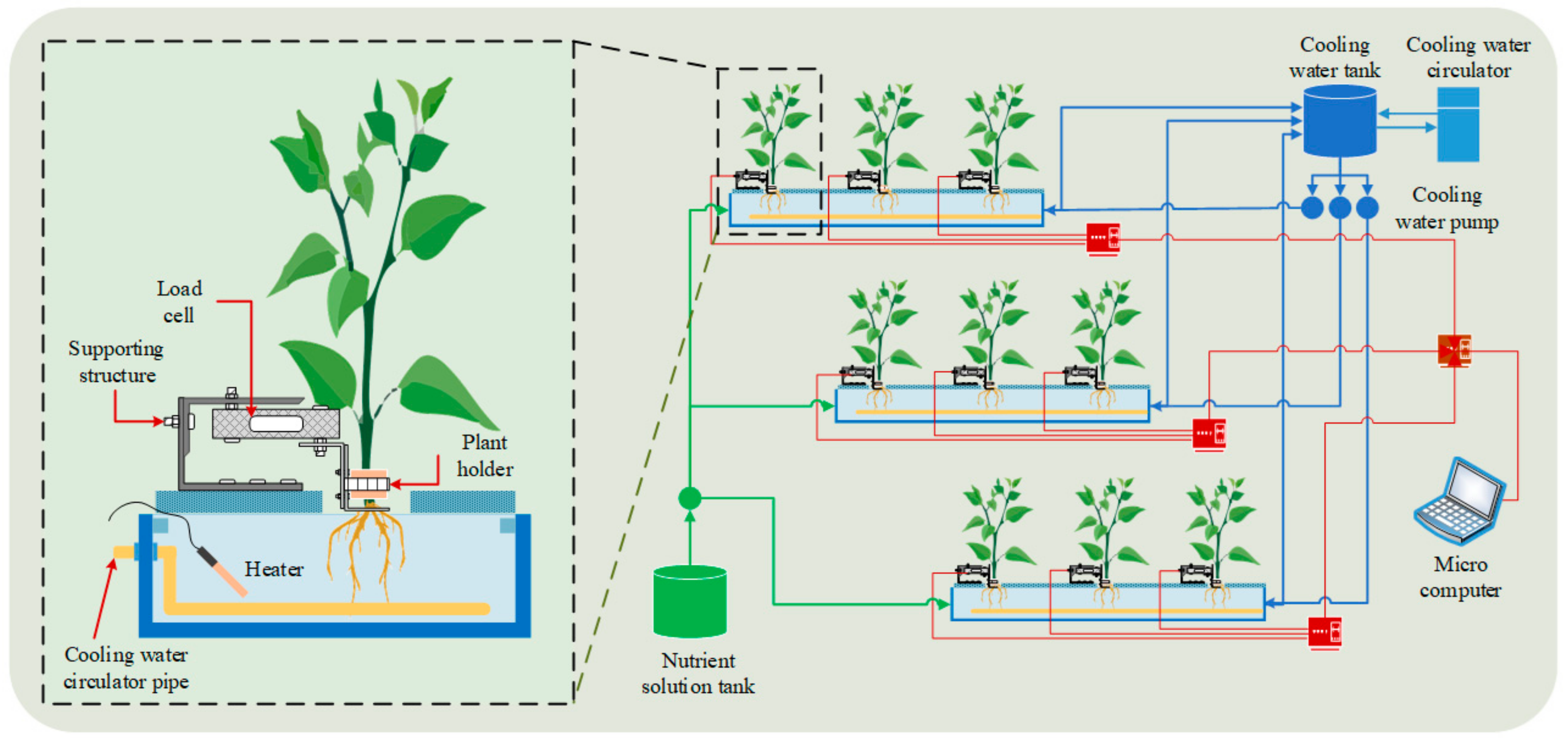
2.2. Experimental Design

At 35 DAS, the plants were transferred to a growth chamber (2.5 × 2.5 × 2 m; (NK System; Nippon Medical and Chemical Instruments Co., Ltd., Osaka, Japan). During observations, the growth chamber was set up consistently with a 12 h photoperiod of 270 µmol m−2 s−1 PPFD (photosynthetic photon flux density) as measured at the base of the growth chamber using a T&D TR-74i illuminance ultraviolet (UV) recorder (T&D Corporation, Matsumoto, Japan), day/night temperature 25/20 ± 1°C, relative humidity 55/70 ± 5%, and nutrient solution 2.3 ± 0.2 dS m−1. Meanwhile, the dissolved oxygen level of the nutrient solution was maintained with the application of an air bubble generator.
To obtain adequate information about the dynamic response of plant growth to RZT, five random patterns of RZT were applied in the range 15–37 °C. Each pattern consisted of three sample plants planted in an independent deep flow technique (DFT) hydroponic system. A total of 15 plants were used for this experiment. To control the RZT, each pattern was equipped with an automatic independent water temperature control system using a NETC-3 thermostat (Newmarins Co. Ltd., Fukuoka, Japan). The thermostat regulated the nutrient solution temperature by controlling a ceramic water heater (Power Safe PRO, Nisso, Japan) and cooling water circulator (FCW-10 Fine Circulators; TGK Co. Ltd., Tokyo, Japan), which circulated cooling water through a copper pipe inside the hydroponic system. To supply the nutrient solution inside the container, an automatic system periodically pumped each container with nutrient solution. The control system is depicted in Figure 1.

2.3. Measurement of Plant Growth

Dynamic changes in plant development were monitored through changes in the fresh weight of the plants during observation. In a controlled environment, the fresh weight of a plant provides useful information on the status of the plant and is also an indicator of plant growth [34,35,36]. In this study, an automated non-destructive plant weight measurement system for pepper plants was developed. The measurement system consisted of a CZL635 micro load cell (loads up to 5 kg and 0.05% precision; Phidgets Inc., Calgary, Canada), load cell support structure, and plant holder, as illustrated in Figure 1. However, because the plant roots were in the nutrient solution, the weight of the plant roots was balanced by buoyant force. Thus, only the weight of the plant shoots was measured. To record the change in plant weight during the experiment, data were sampled at five-minute intervals and stored on a microcomputer (Raspberry Pi 3 Model B+; Raspberry Pi Foundation, Cambridge, UK).
The dynamic response of plant growth was determined as the growth rate of plant weight, which measures the sensitivity of the change in plant weight ( W , [g]) with respect to the change in time ( t , [d]), as shown in the following equation:
W R t = W t

2.4. System Identification Method

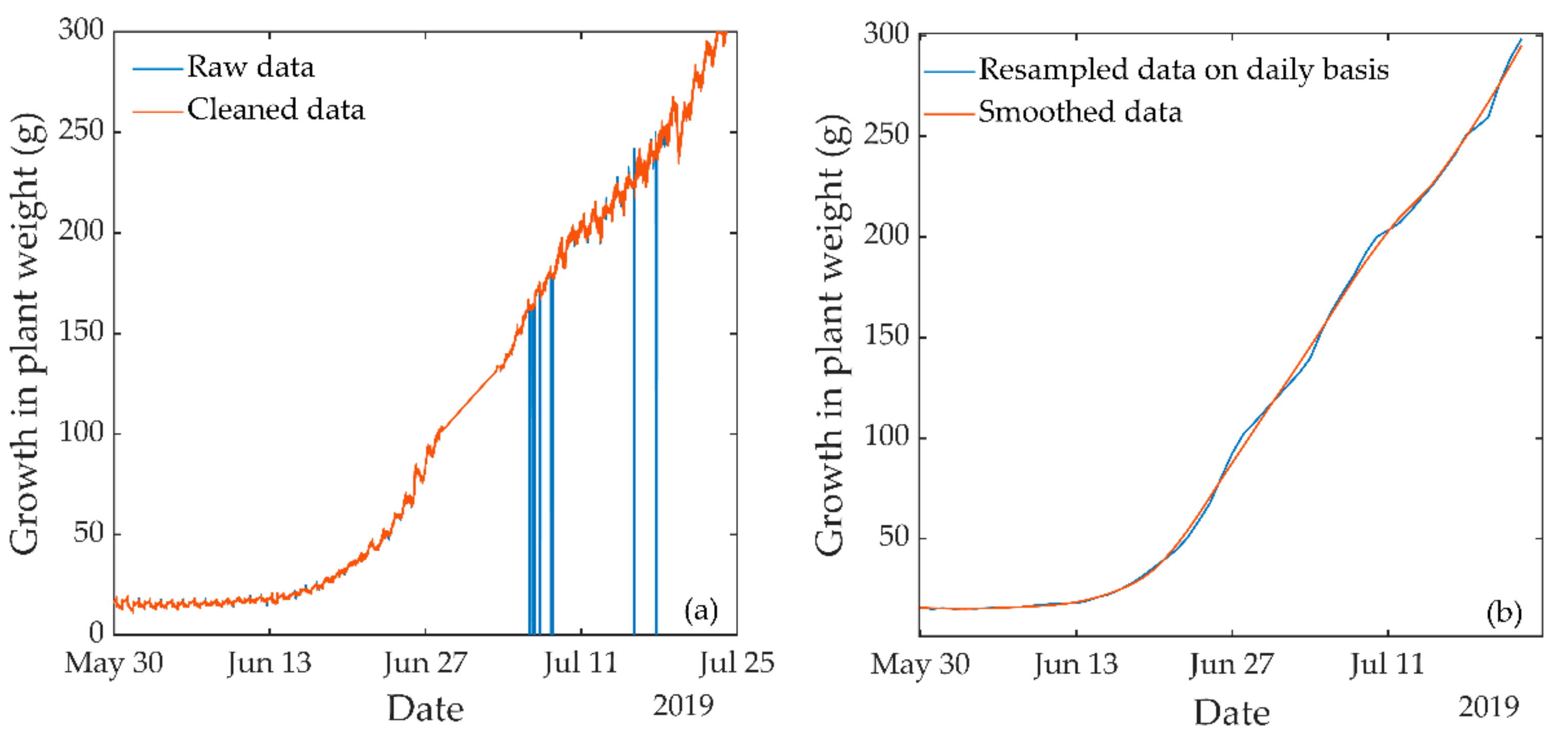
2.4.1. Data Preprocessing

Sensors produce a large number of data points, which can be an advantage in modeling; therefore, these data need to be reliably preprocessed. In supervised learning models, unreliable data could lead to wrong outputs, which affect model performance [37]. Data preprocessing methods were applied in this study to avoid unreliability and to organize data for model development.
Data that deviate considerably from the remaining observations can be defined as outliers. In this study, to detect and remove outliers from time series data, the Hampel Identifier method [38] was applied. The missing data then need to be replaced to maintain completeness and the trend of time series data. Thus, the missing observation data were replaced by the moving average interpolation of their latest neighboring time series data.
The response of plant growth to changes in environmental conditions can be categorized as a long response that can be identified daily. Thus, resampling or aggregation of time series data was needed. In this step, data were resampled on a daily basis using the averaging procedure and then smoothed using the Savitzky–Golay filter [39]. All data preprocessing was performed using the Matlab® Signal Processing Toolbox™ R2019a (MathWorks® Inc., Natick, MA, USA).

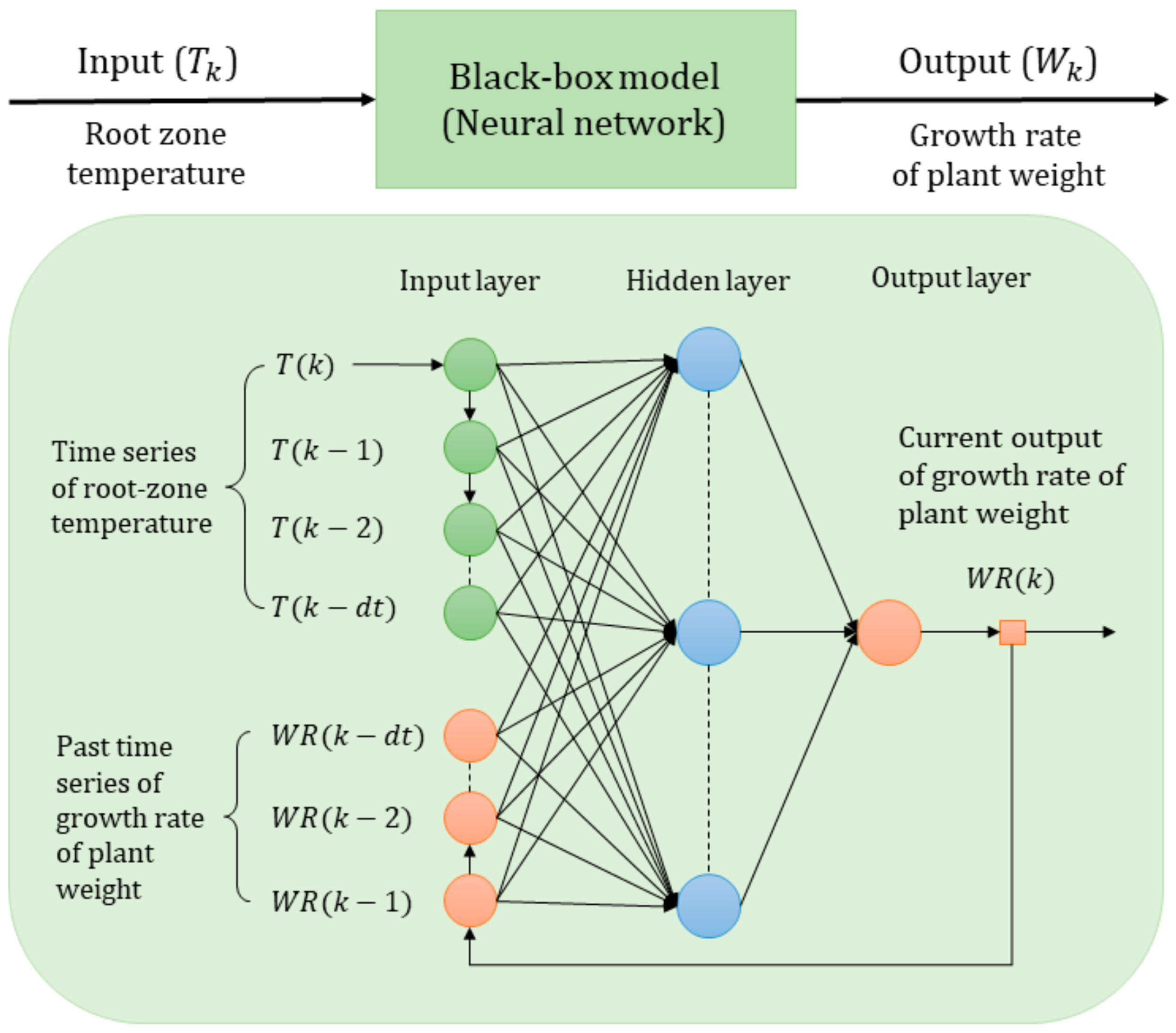
2.4.2. Dynamic Neural Networks for System Identification

In the present study, system identification was considered as a single input–single output system with unknown parameters. Figure 2 shows a block diagram of the SISO system. For the control system of plant growth, the output variable of plant growth response (WR) was estimated from the input variable of RZT (RT).
Artificial neural networks are gaining attention as a general solution for handling non-linear system problems due to their universal approximation capabilities [23]. However, specific neural network architectures are required to solve certain problems optimally. Thus, in recent years, many variants of artificial neural network architecture have been developed. For identification of a dynamic system, in this study, a non-linear autoregressive with exogenous input (NARX) network [40] is considered. NARX networks are a particular class of artificial neural networks characterized by a feedback procedure on the output which can identify any non-linear dynamic system. NARX networks have been employed in various applications of dynamic systems. NARX networks also showed better performance in the prediction of long-term dependencies [41]. Moreover, in particular, for constructing a dynamic model in control system problems, NARX has been widely employed with excellent performance [18,40,42,43,44,45].
The NARX network for identifying the dynamic response of plant growth to RZT and for creating a black box model for simulation is illustrated in Figure 2. In this study, the NARX network structure consists of three layers: input, hidden, and output layers. Moreover, a feedback loop procedure was applied to produce time-series historical input and output data for dynamic identification [23,41].
To identify the dynamic system, the NARX network applies historical input data with time delay ( d t ) operators, T k , T k 1 , , T k d t , and historical output data with time delay operators,   W R k 1 , , G W R k d t , to the input layer, and applies the current output value W R k to the output layer as training signals [23]. Backpropagation with the Levenberg–Marquardt algorithm was then used [46] to train the network. Meanwhile, for prediction, the current output W R k was estimated from historical input data T k , T k 1 , , T k d t and historical output data W R k 1 , , W R k d t , as shown in Equation (2):
W R k = f T k , T k 1 , , T k d t ,   W R k 1 , , W R k d t
A program created using the Matlab® Deep Learning Toolbox™ R2019a (MathWorks® Inc., Natick, MA, USA) was used to develop the model [47]. The workflow of model development in this study is illustrated in Figure 3.

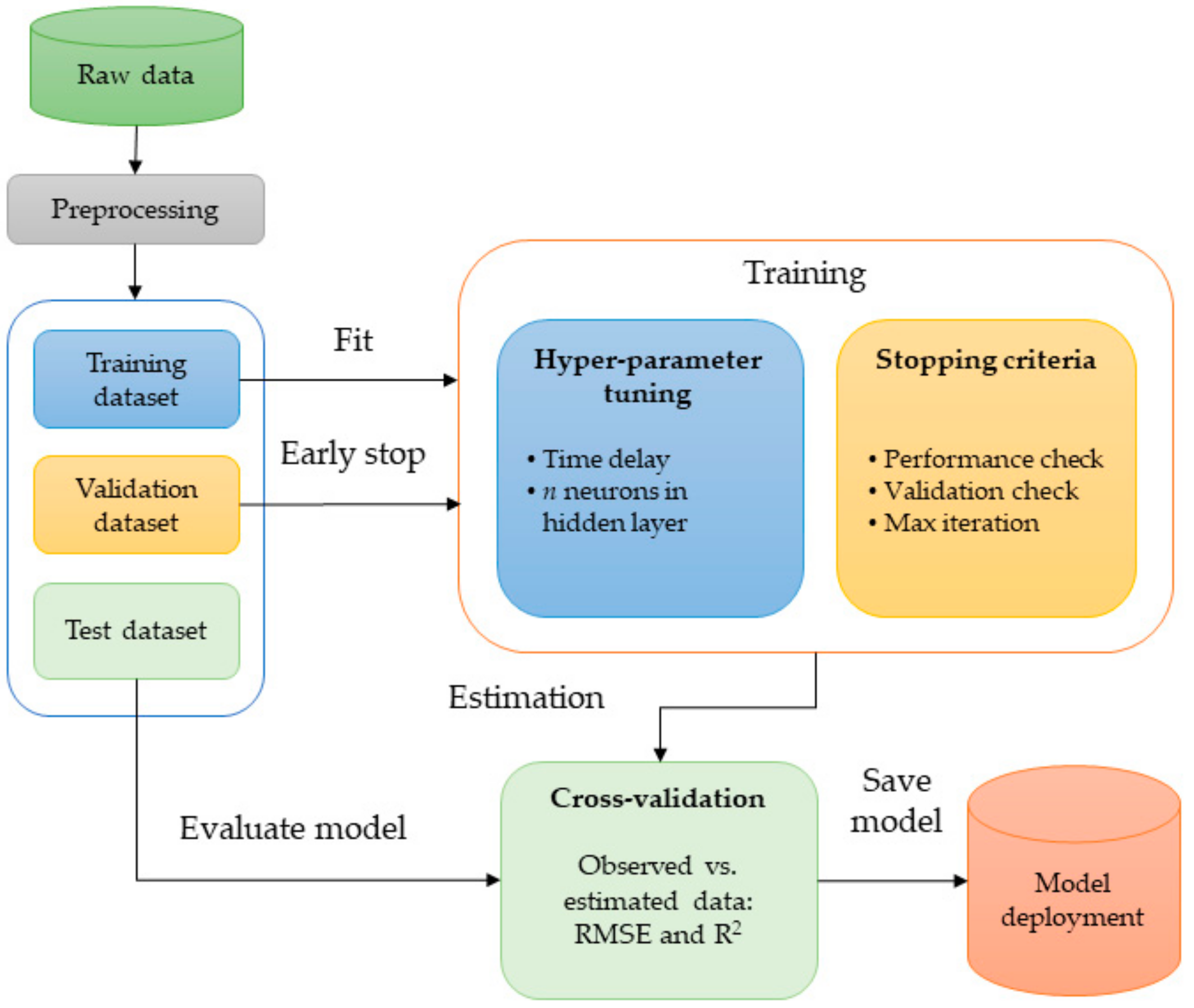
2.4.3. Model Validation and Model Structure Selection

To obtain sufficient accuracy of the identified model, data for identification were divided into three independent datasets: training, validation, and test [48]. The training dataset was the sample of data used by the learning algorithm to fit the model. The trained model was then evaluated using the unbiased validation dataset while tuning the model parameters. During the training process, the validation dataset was also used for regularization by the early stopping training process to prevent model overfitting when generalization was not improving [46]. Four patterns of observation datasets were used for the training and validation datasets, with the proportions of 75 and 25%, respectively. This means that in each dataset, as many as 45 and 15 days of data were used for training and validation, respectively.
Because the structure of the neural network model is significant in the performance of the model, the model parameters, which consist of the time-delay operator and the number of neurons in the hidden layer, needed to be determined. Here, the model parameters were determined through trial and error based on cross-validation. Cross-validation provides an unbiased and robust evaluation of the final model by evaluating the performance of the identified model by comparing the test dataset and estimated data obtained from the model simulation [48].

2.4.4. Model Performance

To measure the performance of the proposed model, two performance criteria were used: the root-mean-squared error (RMSE) and the coefficient of determination ( R 2 ) [48]. The RMSE calculates the error variance of the predicted and observed values (the closer to zero, the better the model performance for RMSE), as shown in Equation (3):
R M S E = 1 n i = 1 n y i y ^ i 2 .
Meanwhile, the coefficient of determination is used to evaluate a model’s ability to explain and predict future outcomes. The value of R 2 ranges from 0 to 1 (the closer to 1, the better the model fits), and is calculated using Equation (4):
R 2 = ( n i = 1 n y ^ i y i i = 1 n y ^ i i = 1 n y i ) 2 n i = 1 n y ^ i 2 ( i = 1 n y ^ i ) 2 n i = 1 n y i 2 ( i = 1 n y i ) 2
where n is the number of data points, y i is the actual value or network output, and y ^ i is the predicted value or network target.

3. Results

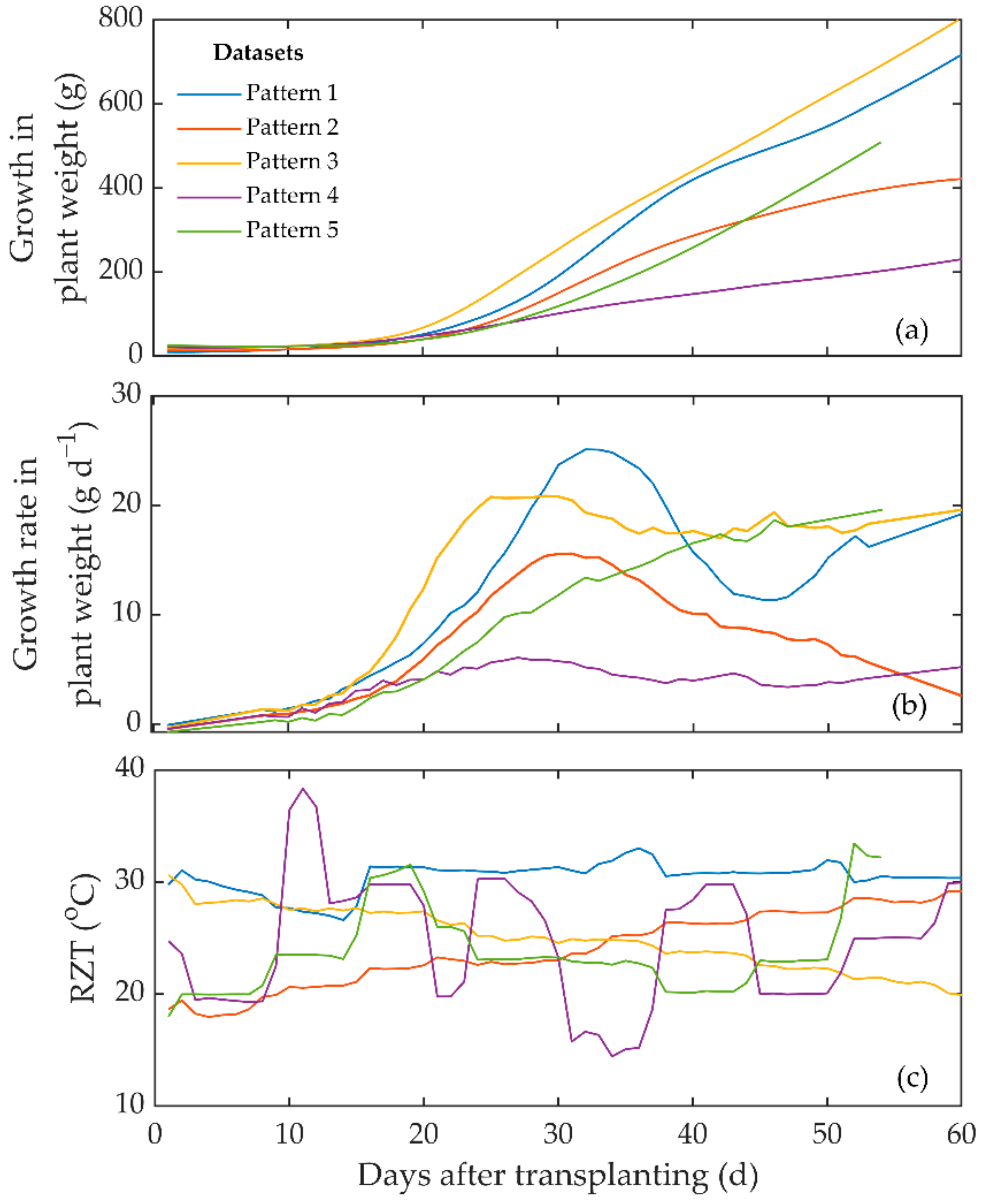
3.1. The Response of Plant Growth to Root Zone Temperature (RZT) for Identification

The time series data of plant weight development were successfully collected using the plant weight measurement system based on a micro load cell. However, much unreliable data were also recorded during observation. Figure 4 shows an example of the raw data from sensor number 14, consisting of numerous suspicious records or outliers. These outliers appeared because of a system error and probably because of unintentional actions, such as unintentional touching of the plants or sensor during observation. The application of data preprocessing effectively removed the unreliable records and reduced the noise from the observed data.
Figure 5 shows daily changes in plant weight, the growth rate of plant weight, and the RZT of hydroponic cultivation for 60 days of observations, which started at 35 days after seeding. These 60 days of observation correspond to the initial stages of pepper plant growth. The data on plant weight are the average values of three pepper plants. Typical patterns of the growth in plant weight under five different RZT treatments are shown. For Pattern 5, however, data were obtained up to only 55 days because of a faulty sensor that produced unreliable records.
In this study, a model was developed based on the measured data for the input and output variables of the system using neural networks. From the observations, the data on growth in plant weight represent the accumulation of plant weight over time. Meanwhile, the growth rate of plant weight measured the sensitivity of the change in plant weight to the change in time, which means that the dynamic effect of RZT treatment on the growth in plant weight can be identified more clearly by using a growth rate variable. Therefore, to achieve a control strategy, the growth rate of plant weight was chosen as the controlled output for neural network model identification.

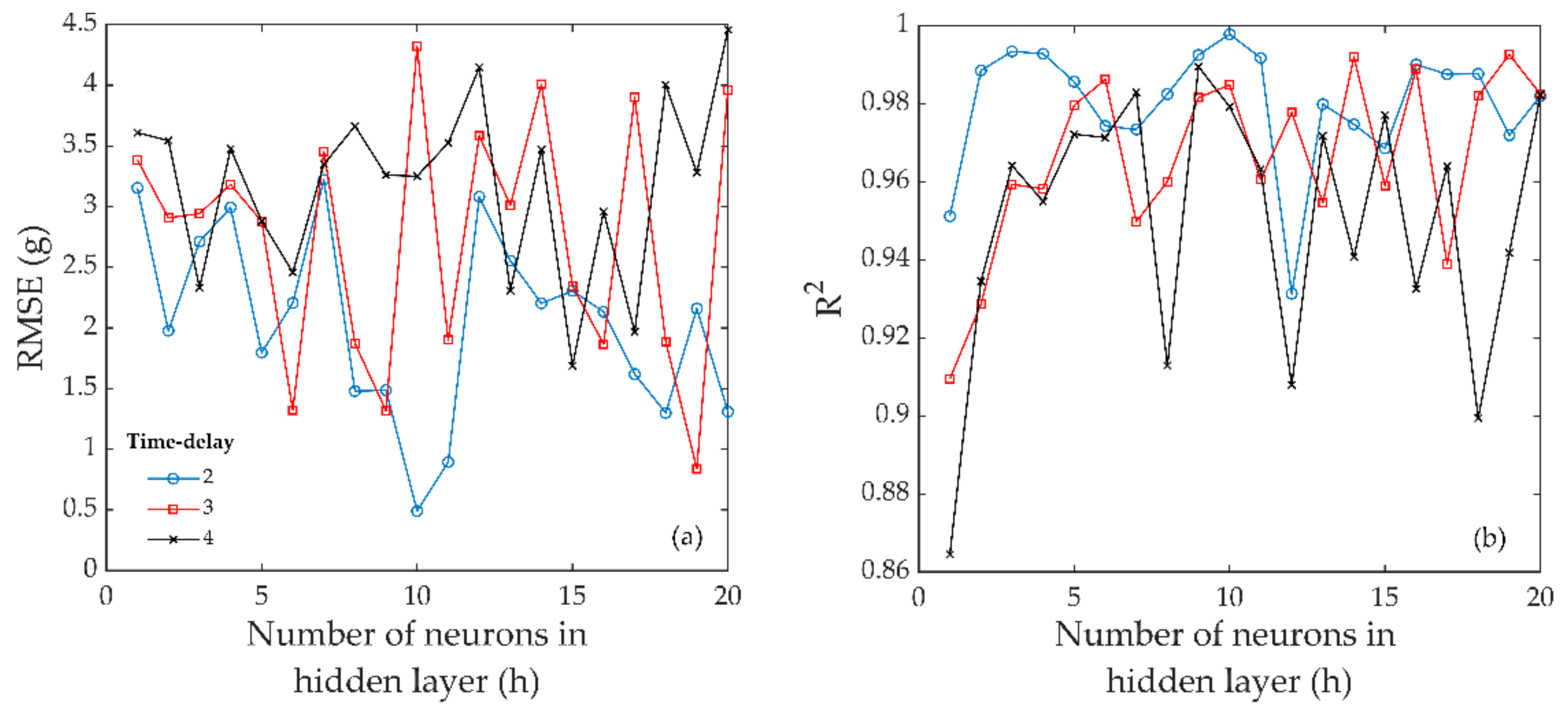
3.2. Determination of the Model Structure

The growth rate of plant weight, as determined by the RZT, was then identified by using neural networks, and a black box model for predicting the growth rate of plant weight was developed. Because the final model structure is determined by the model parameters (dt), which are a combination of time-delay order and the number of neurons in the hidden layer (h), these parameters were determined to find the best performance of the identified model. The effect of the time-delay order and the number of neurons in the hidden layer on model performance was investigated. Figure 6 shows the effect of the model parameters on the estimation error (RMSE). It was found that the RMSE reached its minimal value with the combination of 2 and 10 for the time-delay order and the number of neurons in the hidden layer, respectively. For the second model performance, identical results were obtained, with R2 reaching the best value when the time-delay order and number of neurons in the hidden layer were 2 and 10, respectively. Therefore, the foregoing suggests that the neural network structure with time-delay order dt = 2 and number of neurons in the hidden layer h = 10 is useful for identification.

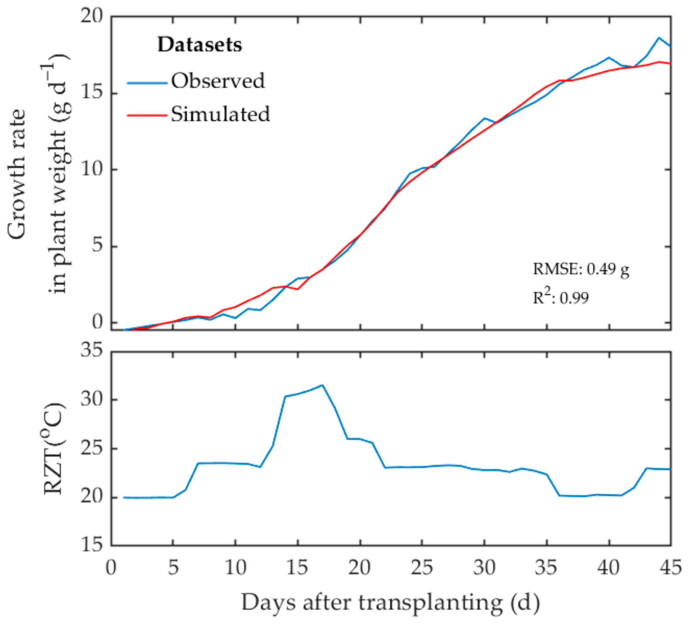
3.3. Identification Results

The performance of the identified neural network model was evaluated by comparing the estimated values and the independent test dataset with the observed values. Figure 7 shows a comparison of the estimated dynamic response calculated by the neural network model and the observed response for the growth rate of plant weight. With RMSE and R2 values of 0.49 g and 0.99, respectively, it was found that the estimated response closely correlated with the observed response.

3.4. Estimation of the Characteristics of Plant Response

Using the identified neural network model, the relationship between RZT and the response of plant growth was then estimated to provide an insight into the basic properties of the dynamic system model. Figure 8 shows the estimated step response of the growth rate of plant growth to stepped input from 20 to 21, 23, 25, 27, and 29 °C. In general, the step responses dramatically increased as the step input of RZT increased. However, through the given range of five step inputs, the dynamic system model generated five different characteristics of the step response. The gain of step response from 20 to 21 °C was slightly faster, but then immediately steady. Meanwhile, the gains of step response from 20 to 23 °C and 20 to 25 °C were largest. In general, with change in the input variable of RZT, the gain in the step response of growth rate in plant weight gradually increased with time. These results show how the model simulates the dynamic characteristics of step response for different input conditions, which illustrates the ability of RZT in various ranges to control plant growth in a dynamic system.

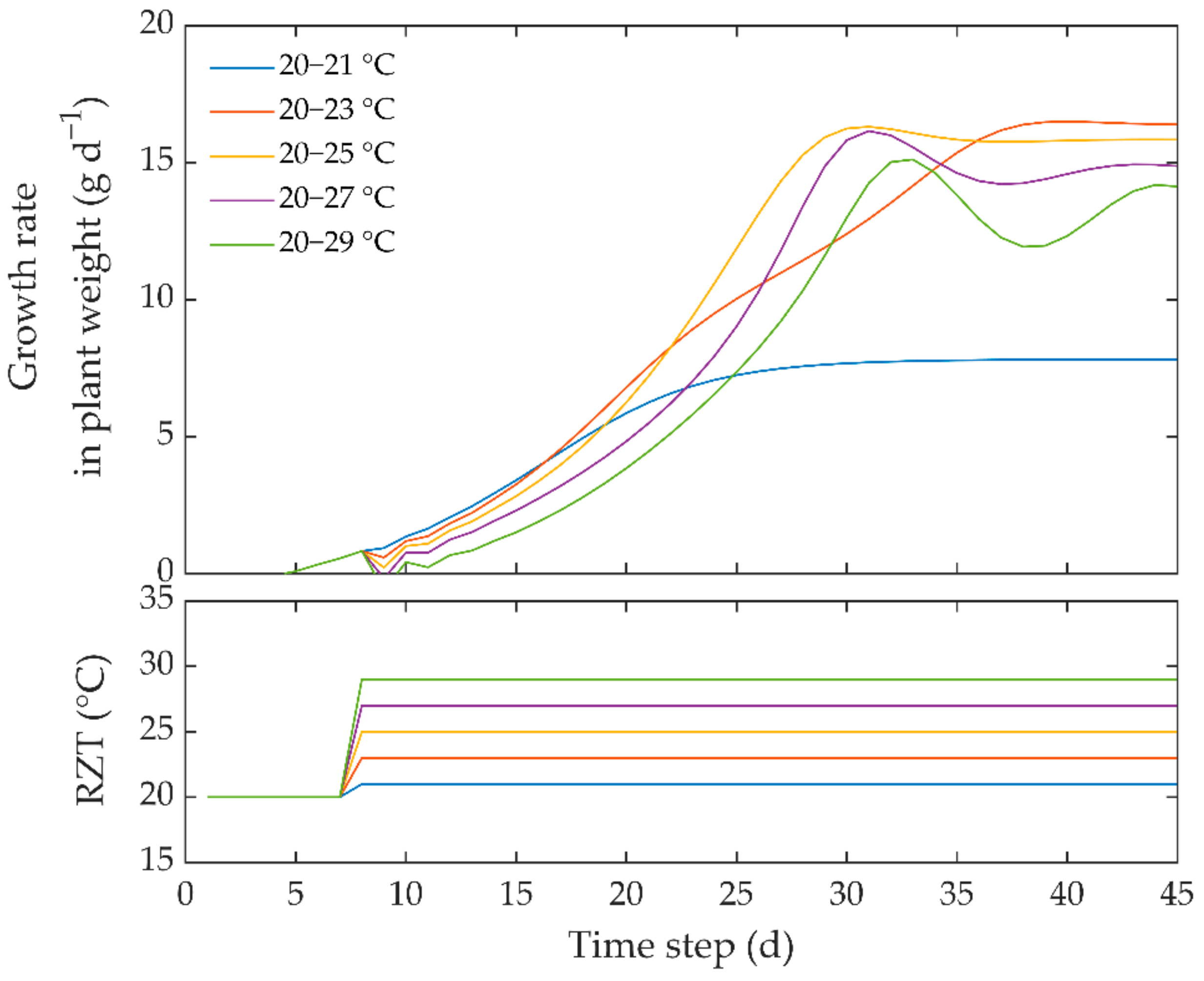
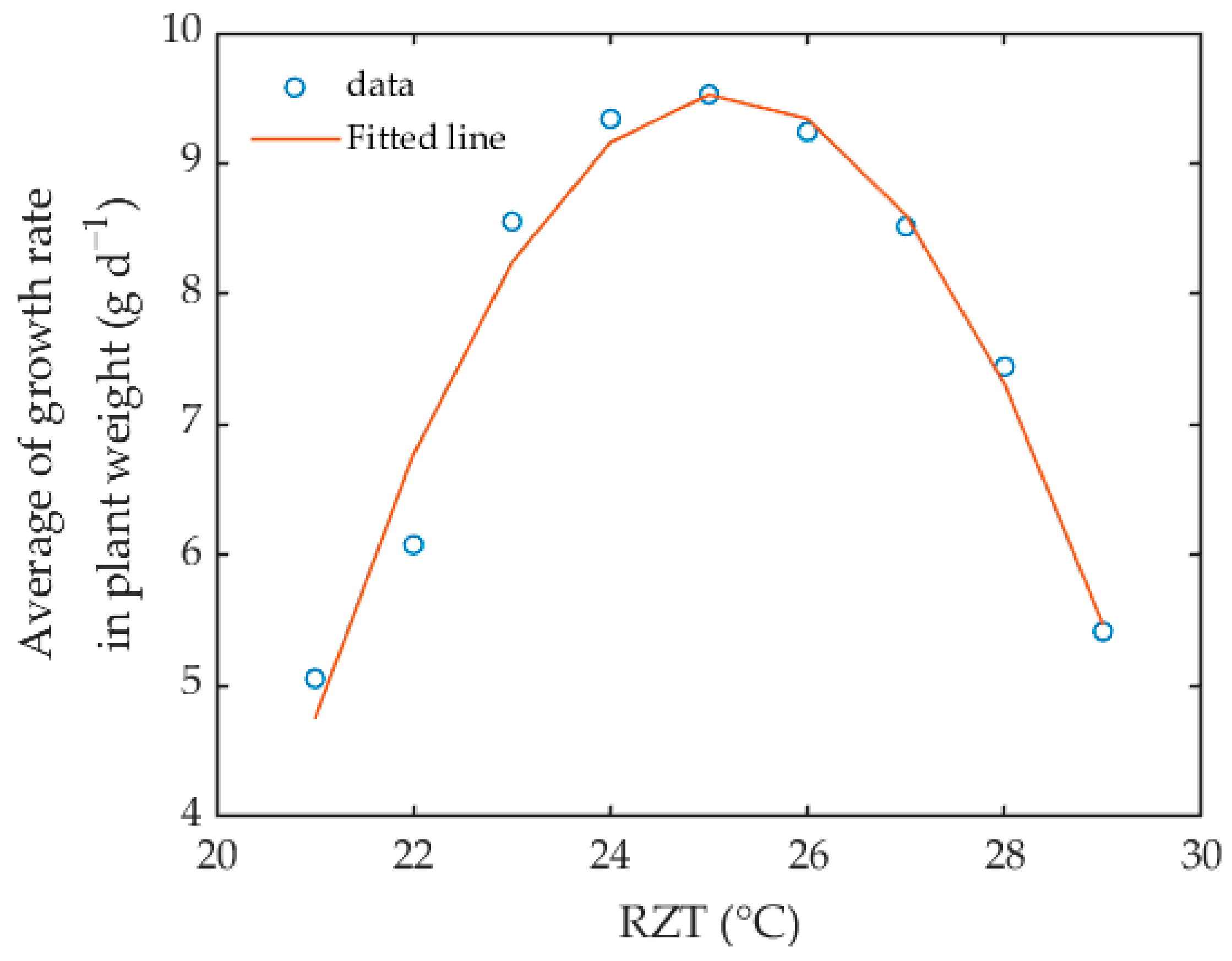
3.5. Estimation of the Relationship between RZT and the Growth Rate of Plant Weight

In order to confirm the relevance of the model in this study, the estimated relationship between RZT and the average growth rate in plant weight, which also represents plant growth, was examined via model simulation. Figure 9 shows the estimated static relationship between RZT and the growth rate of plant weight. The estimated value of the growth rate of plant weight was obtained from the average of the step response calculated using the identified model, where the step input value was set as stationary from various values. From the simulation, it can be seen that the growth rate of plant weight increased with RZT. However, above the range 25 to 26 °C, the growth rate tended to decrease with RZT. In general, it was found that the relationship between RZT and the growth rate of the plant showed strong non-linearity and peaked in the range of 24 to 26 °C. This result is consistent with a previous study which reported that the optimal RZT range for bell pepper (Capsicum annum L.) is in the range 25 to 27 °C or less in terms of yield [49] and 24 °C in terms of shoot dry weight [50].

4. Discussion and Conclusions

In this study, the dynamic responses of plant growth as affected by changes in the RZT were examined using an automatic plant weight measurement system based on a load cell. Since plant tissue is composed mostly of water, the fresh weight of a plant is very sensitive to changes in environmental conditions. For this reason, in order to examine the fundamental eco-physiological behavior of the response of plant growth to RZT, experiments were conducted in a strictly controlled environment using a growth chamber, where light intensity, temperature, and relative humidity were controlled precisely. As the environmental conditions inside the growth chamber were maintained constant, it can be assumed that the responses of plant growth were affected by the changes in RZT.
Then, an artificial neural network was used to construct a dynamic model of the responses of plant growth as affected by changes in the RZT in hydroponic cultivation. Based on the examination, it was found that the NARX networks presented in this study were useful in identifying the complex process of the dynamic response of plant growth as affected by changes in the RZT over 45 days of cultivation. The NARX networks were shown to be capable of performing long-term dependency prediction, as also shown by [40,41]. The model also successfully performed step response simulation, which is typically conducted in control studies to estimate the basic properties of a dynamic system [19]. This suggests that dynamic optimization can potentially be applied to the system in order to maximize plant growth. Moreover, from the simulation, estimation of the static relationship between the response of plant growth and RZT can also be generated. The static relationship was determined as having strong non-linearity with an upside-down parabolic curve peaking in the range of 24 to 26 °C, which is consistent with previous studies on the relationship of plant growth and RZT [49,50]. This suggests that a reliable computational model can be useful to predict the dynamic behavior of plant growth as affected by RZT.
In previous studies, the examination of dynamic plant growth control using root zone environmental factors in hydroponic cultivation was limited to nutrient solution concentration [16]. Meanwhile, optimal temperature control of the root zone environment, which is one of the essential determining factors in hydroponic cultivation, had not been thoroughly investigated [18]. Identification of the dynamic responses of plant growth as affected by RZT, which was conducted in this study, may be useful for a better understanding of plant growth control in plant production systems.
However, the artificial neural network model presented in this study cannot be applied in cultivation systems as it is. This is because the model is limited to the specific range of environmental conditions in the setup used during the experiment. More data on plant response in broader environmental conditions are required to construct a more robust model. For an artificial neural network model, more training data are better for identification. Given that one of the significant advantages of an artificial neural network model is the ability to re-train the current model using new data, this model has great potential for further development.

Author Contributions

Conceptualization, G.K.A., K.H. and T.M.; methodology, G.K.A., K.H. and T.M.; software, G.K.A.; formal analysis, G.K.A.; investigation, G.K.A.; resources, K.H. and T.M.; data curation, G.K.A.; writing—original draft preparation G.K.A.; writing—review and editing, G.K.A.; visualization, G.K.A.; supervision, K.H. and T.M. All authors have read and agreed to the published version of the manuscript.

Acknowledgments

The first author would like to thank the Indonesia Endowment Fund for Education (LPDP), Ministry of Finance and Ministry of Research, Technology and Higher Education of the Republic of Indonesia for their support of his study.

Conflicts of Interest

The authors declare no conflict of interest.

References

  1. Sambo, P.; Nicoletto, C.; Giro, A.; Pii, Y.; Valentinuzzi, F.; Mimmo, T.; Lugli, P.; Orzes, G.; Mazzetto, F.; Astolfi, S.; et al. Hydroponic Solutions for Soilless Production Systems: Issues and Opportunities in a Smart Agriculture Perspective. Front. Plant Sci. 2019, 10, 923. [Google Scholar] [CrossRef] [PubMed]
  2. He, J. Root Growth, Morphological and Physiological Characteristics of Subtropical and Temperate Vegetable Crops Grown in the Tropics Under Different Root-Zone Temperature. In Plant Growth; Rigobelo, E.C., Ed.; IntechOpen: London, UK, 2016; pp. 131–148. [Google Scholar]
  3. Mortensen, L.M. Growth Responses of Some Greenhouse Plants to Environment. II. The Effect of Soil Temperature on Chrysanthemum Morifolium Ramat. Sci. Hortic. (Amsterdam) 1982, 16, 47–55. [Google Scholar] [CrossRef]
  4. Gosselin, A.; Trudel, M.J. Interactions between Air and Root Temperatures on Greenhouse Tomato: II. Mineral Composition of Plants. J. Amer. Soc. Hort. Sci. 1983, 108, 905–909. [Google Scholar]
  5. Ingram, D.L.; Ruter, J.M.; Martin, C.A. Review: Characterization and Impact of Supraoptimal Root-Zone Temperatures in Container-Grown Plants. HortScience 2015, 50, 530–539. [Google Scholar] [CrossRef] [Green Version]
  6. Kawasaki, Y.; Matsuo, S.; Suzuki, K.; Kanayama, Y.; Kanahama, K. Root-Zone Cooling at High Air Temperatures Enhances Physiological Activities and Internal Structures of Roots in Young Tomato Plants. J. Jpn. Soc. Hortic. Sci. 2013, 82, 322–327. [Google Scholar] [CrossRef] [Green Version]
  7. Kawasaki, Y.; Matsuo, S.; Kanayama, Y.; Kanahama, K. Effect of Root-Zone Heating on Root Growth and Activity, Nutrient Uptake, and Fruit Yield of Tomato at Low Air Temperatures. J. Jpn. Soc. Hortic. Sci. 2014, 83, 295–301. [Google Scholar] [CrossRef] [Green Version]
  8. Morimoto, T.; Hashimoto, Y.; Fukuyama, T. Identification and Control of Hydroponic System in Greenhouses. IFAC Proc. Vol. 1985, 18, 1689–1693. [Google Scholar] [CrossRef]
  9. Morimoto, T.; Hashimoto, Y. Speaking Plant/Fruit Approach for Greenhouses and Plant Factories. Environ. Control. Biol. 2009, 47, 55–72. [Google Scholar] [CrossRef]
  10. Hashimoto, Y. Recent Strategies of Optimal Growth Regulation By the Speaking Plant Concept. Acta Hortic. 1989, 260, 115–122. [Google Scholar] [CrossRef]
  11. Morimoto, T.; Hatou, K.; Hashimoto, Y. Intelligent Control for a Plant Production System. Control. Eng. Pract. 1996, 4, 773–784. [Google Scholar] [CrossRef]
  12. Nishina, H. Development of Speaking Plant Approach Technique for Intelligent Greenhouse. Agric. Agric. Sci. Procedia 2015, 3, 9–13. [Google Scholar] [CrossRef] [Green Version]
  13. Morimoto, T.; Hashimoto, Y. An Intelligent Control for Greenhouse Automation, Oriented by the Concepts of SPA and SFA—An Application to a Post-Harvest Process. Comput. Electron. Agric. 2000, 29, 3–20. [Google Scholar] [CrossRef]
  14. Morimoto, T.; Hashimoto, Y. AI Approaches to Identification and Control of Total Plant Production Systems. Control. Eng. Pract. 2000, 8, 555–567. [Google Scholar] [CrossRef]
  15. Fasol, K.H.; Jörgl, H.P. Principles of Model Building and Identification. Automatica 1980, 16, 505–518. [Google Scholar] [CrossRef]
  16. Yumeina, D.; Morimoto, T. Dynamic Optimization of Solution Nutrient Concentration to Promote the Initial Growth of Tomato Plants in Hydroponics. Environ. Control. Biol. 2014, 52, 87–94. [Google Scholar] [CrossRef] [Green Version]
  17. Morimoto, T.; Takeuchi, T.; Hashimoto, Y. Growth Optimization of Plant by Means of the Hybrid System of Genetic Algorithm and Neural Network. In Proceedings of the 1993 International Conference on Neural Networks, Nagoya, Japan, 25–29 October 1993; IEEE: Piscataway, NJ, USA, 1993; Volume 3, pp. 2979–2982. [Google Scholar]
  18. Yumeina, D.; Aji, G.K.; Morimoto, T. Dynamic Optimization of Water Temperature for Maximizing Leaf Water Content of Tomato in Hydroponics Using an Intelligent Control Technique. Acta Hortic. 2017, 1154, 55–64. [Google Scholar] [CrossRef]
  19. Isermann, R.; Münchhof, M. Identification of Dynamic Systems: An Introduction with Applications, 1st ed.; Springer-Verlag: Berlin/Heidelberg, Germany, 2011. [Google Scholar]
  20. Whittaker, A.D.; Thieme, R.H. Editorial: Integration of Knowledge Systems into Agricultural Problem Solving. Comput. Electron. Agric. 1990, 4, 271–273. [Google Scholar] [CrossRef]
  21. Yin, X.; Laar, H.H. Van. Crop. Systems Dynamics: An. Ecophysiological Simulation Model. for Genotype-by-Environment Interactions, 1st ed.; Wageningen Academic Publishers: Wageningen, The Netherlands, 2005. [Google Scholar]
  22. Carson, E.; Feng, D.D.; Pons, M.N.; Soncini-Sessa, R.; van Straten, G. Dealing with Bio- and Ecological Complexity: Challenges and Opportunities. Annu. Rev. Control. 2006, 30, 91–101. [Google Scholar] [CrossRef]
  23. Isermann, R.; Ernst, S.; Nelles, O. Identification with Dynamic Neural Networks—Architectures, Comparisons, Applications. IFAC Proc. Vol. 1997, 30, 947–972. [Google Scholar] [CrossRef]
  24. Hinton, G.E. How Neural Networks Learn from Experience. Sci. Am. 1992, 267, 144–151. [Google Scholar] [CrossRef]
  25. Rumelhart, D.E.; Hinton, G.E.; Williams, R.J. Learning Internal Representations by Error Propagation. In Readings in Cognitive Science: A Perspective from Psychology and Artificial Intelligence; Morgan Kaufmann Publishers, Inc.: San Mateo, CA, USA, 1988; pp. 399–421. [Google Scholar]
  26. Sablani, S.S.; Datta, A.K.; Rahman, M.S.; Mujumdar, A.S. Handbook of Food and Bioprocess. Modeling Techniques; Sablani, S., Datta, A., Shafiur Rehman, M., Mujumdar, A., Eds.; CRC Press: Boca Raton, FL, USA, 2006; Volume 20065751. [Google Scholar]
  27. Liakos, K.G.; Busato, P.; Moshou, D.; Pearson, S.; Bochtis, D. Machine Learning in Agriculture: A Review. Sensors 2018, 18, 2674. [Google Scholar] [CrossRef] [PubMed] [Green Version]
  28. Islam, M.P.; Morimoto, T.; Hatou, K. Dynamic Optimization of inside Temperature of Zero Energy Cool Chamber for Storing Fruits and Vegetables Using Neural Networks and Genetic Algorithms. Comput. Electron. Agric. 2013, 95, 98–107. [Google Scholar] [CrossRef]
  29. FAO. Good Agricultural Practices for Greenhouse Vegetable Production in the South. East. European Countries; FAO: Rome, Italy, 2017. [Google Scholar]
  30. Erickson, A.N.; Markhart, A.H. Flower Developmental Stage and Organ Sensitivity of Bell Pepper (Capsicum annuum L.) to Elevated Temperature. Plant. Cell Environ. 2002, 25, 123–130. [Google Scholar] [CrossRef]
  31. Pressman, E.; Shaked, R.; Firon, N. Exposing Pepper Plants to High Day Temperatures Prevents the Adverse Low Night Temperature Symptoms. Physiol. Plant. 2006, 126, 618–626. [Google Scholar] [CrossRef]
  32. Bosland, P.W.; Votava, E.J. Introduction. In Peppers: Vegetable and spice capsicums; CABI: Wallingford, UK, 2012; pp. 1–12. [Google Scholar]
  33. Aloni, B.; Karni, L.; Daie, J. Effect of Heat Stress on the Growth, Root Sugars, Acid Invertase and Protein Profile of Pepper Seedlings Following Transplanting. J. Hortic. Sci. 1992, 67, 717–725. [Google Scholar] [CrossRef]
  34. Oda, M.; Tsuji, K. Monitoring Fresh Weight of Leaf Lettuce. Jpn. Agric. Res. Q. 1992, 25, 19–25. [Google Scholar]
  35. Chen, W.-T.; Yeh, Y.-H.F.; Liu, T.-Y.; Lin, T.-T. An Automated and Continuous Plant Weight Measurement System for Plant Factory. Front. Plant. Sci. 2016, 7, 392. [Google Scholar] [CrossRef] [Green Version]
  36. Helmer, T.; Ehret, D.L.; Bittman, S. CropAssist, an Automated System for Direct Measurement of Greenhouse Tomato Growth and Water Use. Comput. Electron. Agric. 2005, 48, 198–215. [Google Scholar] [CrossRef]
  37. Wong, W.K.; Guo, Z.X. Intelligent Sales Forecasting for Fashion Retailing Using Harmony Search Algorithms and Extreme Learning Machines. In Optimizing Decision Making in the Apparel Supply Chain Using Artificial Intelligence (AI); Woodhead Publishing Limited: Sawston, UK, 2013; pp. 170–195. [Google Scholar] [CrossRef]
  38. Davies, L.; Gather, U. The Identification of Multiple Outliers. J. Am. Stat. Assoc. 1993, 88, 782–792. [Google Scholar] [CrossRef]
  39. Dai, W.; Selesnick, I.; Rizzo, J.-R.; Rucker, J.; Hudson, T. A Nonlinear Generalization of the Savitzky-Golay Filter and the Quantitative Analysis of Saccades. J. Vis. 2017, 17, 10. [Google Scholar] [CrossRef]
  40. Siegelmann, H.T.; Horne, B.G.; Giles, C.L. Computational Capabilities of Recurrent NARX Neural Networks. IEEE Trans. Syst. Man Cybern. Part. B 1997, 27, 208–215. [Google Scholar] [CrossRef] [PubMed] [Green Version]
  41. Menezes, J.M.P.; Barreto, G.A. Long-Term Time Series Prediction with the NARX Network: An Empirical Evaluation. Neurocomputing 2008, 71, 3335–3343. [Google Scholar] [CrossRef]
  42. Mohd, N.; Aziz, N. Performance and Robustness Evaluation of Nonlinear Autoregressive with Exogenous Input Model Predictive Control in Controlling Industrial Fermentation Process. J. Clean. Prod. 2016, 136, 42–50. [Google Scholar] [CrossRef]
  43. Ng, B.C.; Darus, I.Z.M.; Jamaluddin, H.; Kamar, H.M. Dynamic Modelling of an Automotive Variable Speed Air Conditioning System Using Nonlinear Autoregressive Exogenous Neural Networks. Appl. Therm. Eng. 2014, 73, 1253–1267. [Google Scholar] [CrossRef]
  44. Chan, R.W.K.; Yuen, J.K.K.; Lee, E.W.M.; Arashpour, M. Application of Nonlinear-Autoregressive-Exogenous Model to Predict the Hysteretic Behaviour of Passive Control Systems. Eng. Struct. 2015, 85, 1–10. [Google Scholar] [CrossRef]
  45. Mai, C.V.; Spiridonakos, M.D.; Chatzi, E.N.; Sudret, B. Surrogate Modeling for Stochastic Dynamical Systems by Combining Nonlinear Autoregressive with Exogenous Input Models and Polynomial Chaos Expansions. Int. J. Uncertain. Quantif. 2016, 6, 313–339. [Google Scholar] [CrossRef]
  46. Beale, M.H.; Hagan, M.T.; Demuth, H.B. Neural Network Toolbox (TM) User’s Guide; The MathWorks, Inc.: Natick, MA, USA, 2016. [Google Scholar]
  47. Aji, G.K.; Hatou, K.; Morimoto, T. Matlab Program Script for Modeling the Dynamic Response of Plant Growth to Root Zone Temperature in Hydroponic Chili Pepper Plant using Neural Network. Available online: https://github.com/mradjie/narx-plant-growth. (accessed on 25 May 2020).
  48. Kuhn, M.; Johnson, K. Applied Predictive Modeling; Springer: New York, NY, USA, 2013. [Google Scholar]
  49. Díaz-Pérez, J.C. Bell Pepper (Capsicum annum L.) Grown on Plastic Film Mulches: Effects on Crop Microenvironment, Physiological Attributes, and Fruit Yield. HortScience 2010, 45, 1196–1204. [Google Scholar] [CrossRef] [Green Version]
  50. Gosselin, A.; Trudel, M.J. Root-Zone Temperature Effects on Pepper. J. Am. Soc. Hort. Sci. 1986, 111, 220–224. [Google Scholar]
Figure 1. Root zone temperature control system and plant growth measuring system using a load cell sensor.
Agriculture 10 00234 g001
Figure 2. Block diagram of the single input–single output (SISO) system for system identification, and non-linear autoregressive with exogenous input (NARX) network structure with three layers, one input time series of the root zone temperature T k , one hidden layer (h), one output time series of the growth rate of plant weight W R k , and a time-delay ( d t )   neural network for identifying a dynamic model.
Agriculture 10 00234 g002
Figure 3. The workflow of model development using NARX neural networks.
Agriculture 10 00234 g003
Figure 4. Sample preprocessing of observation data from sensor 14: (a) the original data were cleaned of unreliable records using the Hampel Identifier and reconstructed using the moving average method; (b) the cleaned data were then resampled on a daily basis and smoothed using the Savitzky–Golay filter.
Agriculture 10 00234 g004
Figure 5. Typical daily change in plant weight (a), the growth rate in plant weight (b), and the RZT (c) in hydroponic pepper cultivation.
Agriculture 10 00234 g005
Figure 6. The relationship between the time-delay order (dt), the number of neurons in the hidden layer (h), and model performances: (a) root-mean-squared error (RMSE) and (b) R2.
Agriculture 10 00234 g006
Figure 7. Comparison of the estimated response calculated by the developed neural network model and the observed growth rate of plant weight.
Agriculture 10 00234 g007
Figure 8. Estimated step response of the growth rate of plant weight to stepped RZT input, obtained via simulation.
Agriculture 10 00234 g008
Figure 9. The estimated static relationship between the growth rate of plant weight and RZT, obtained via simulation.
Agriculture 10 00234 g009

