
Impact of Agricultural Practices on Water Quality of Old Woman Creek Watershed, Ohio


1
Texas Institute for Applied Environmental Research (TIAER), Tarleton State University, Member of The Texas A&M University System, Stephenville, TX 76401, USA
2
Norwegian Institute of Bioeconomy Research, 1430 Ås, Norway
3
Department of Geology, Kent State University, Kent, OH 44240, USA
*
Author to whom correspondence should be addressed.
Agriculture 2021, 11(5), 426; https://0-doi-org.brum.beds.ac.uk/10.3390/agriculture11050426
Submission received: 15 April 2021
/
Accepted: 3 May 2021
/
Published: 9 May 2021
Abstract
:The effect of agricultural practices on water quality of Old Woman Creek (OWC) watershed was evaluated in a hydrological model using the Parameter-elevation Regressions on Independent Slopes Model (PRISM) climate data and 20 different global circulation models (GCMs) from the Coupled Model Intercomparison Project Phase 5 (CMIP5). A hydrological model was set up in the Soil and Water Assessment Tool (SWAT), while calibration was done using a Multi-Objective Evolutionary Algorithm and Pareto Optimization with PRISM climate data. Validation was done using the measured data from the USGS gage station at Berlin Road in the OWC watershed and water quality data were obtained from the water quality lab, Heidelberg University. Land use scenario simulations were conducted by varying percentages of agricultural land from 20% to 40%, 53.5%, 65%, and 80% while adjusting the forest area. A total of 105 simulations was run for the period 2015–2017: one with PRISM data and 20 with CMIP5 model data for each of the five land use classes scenarios. Ten variables were analyzed, including flow, sediment, organic nitrogen, organic phosphorus, mineral phosphorus, chlorophyll a, CBOD, dissolved oxygen, total nitrogen, and total phosphorus. For all the variables of interest, the average of the 20 CMIP5 simulation results show good correlation with the PRISM results with an underestimation relative to the PRISM result. The underestimation was insignificant in organic nitrogen, organic phosphorus, total nitrogen, chlorophyll a, CBOD, and total phosphorus, but was significant in CMIP5 flow, sediment, mineral phosphorus, and dissolved oxygen. A weak negative correlation was observed between agricultural land percentages and flow, and between agricultural land percentages and sediment, while a strong positive correlation was observed between agricultural land use and the water quality variables. A large increase in farmland will produce a small decrease in flow and sediment transport with a large increase in nutrient transport, which would degrade the water quality of the OWC estuary with economic implications.
1. Introduction
Agricultural nonpoint pollution occurs when runoff generated from excessive precipitation washes away the agricultural land surfaces into nearby waterbodies. Tillage operations affect the availability of nutrients and soil particles for erosion. The runoff generated carries nutrients from fertilizers and natural pollution sources into nearby water bodies, thereby increasing the water turbidity. The water quality of the aquatic setting is influenced by the influx of nutrients due to anthropogenic activities [1]. The integrated effect of soil types, weather, and management practices may increase nutrient influx, which may lead to eutrophication [1]. Research in water quality have recently shifted to the use of physical models using geospatial data to identify and analyze the point and nonpoint pollutants and to simulate their extent [2,3]. Global warming is predicted to change the meteorological elements, thereby affecting the watershed nutrients mechanisms [1].
The study of the impact of climate change and land use on watershed hydrology and surface water availability can be done using hydrological models [4]. Models that have proven to be efficient at a watershed scale are the Soil and Water Assessment Tool (SWAT) [5], Hydrologic Simulation Program Fortran (HSPF) [6], and Better Assessment Science Integrating Point and Non-point Sources (BASINS) [7]. The knowledge obtained from the modeling work provide environmental planners with short- and long-term consequences of management practices which helps to institute methods of reducing pollution [3]. Woznicki and Nejadhashemi [8] reported an increase in sediment transport, total phosphorus, and total nitrogen with a future climate change model in SWAT. In the SWAT hydrological modeling of the Maumee River basin conducted by Michalak et al. [9], it was recommended that the estimated increase in sediment and nutrient transport associated with the projected climate change could be reduced by Best Management Practices (BMPs).
Khanna et al. [10] created hydrological and economic models to simulate the reduction in the effect of sediment and nutrient transport from agricultural fields on water quality, thereby improving the habitat conditions for wildlife. This method involved reduction in sediment loadings by retiring the most erosion sensitive cropland areas, as stipulated in the Conservation Reserve Enhancement Program (CREP). They presented an analytical structure for an economical means of land enrollment in the CREP program. In Du et al. [11], a SWAT model of the Dagu River basin in China was used to assess the impact of variable climate conditions and land use on runoff and it was discovered that the impact of climate was greater than that of land use. Scavia et al. [12] used a multi-model approach consisting of five different models built on the same SWAT platform with different data sources, model set up, parameterization, management practices, and calibration conditions to evaluate the reduction in nutrient transport into the Maumee River watershed. In validation, they found a good agreement between the weighted average of the five models and the observed measurement with acceptable inter-model variability.
The goal of this work was to determine the responses of flow and water quality variables to changes in land use/land cover (LULC) in the Old Woman Creek (OWC) watershed. The objectives were to develop a hydrological model for the OWC watershed using SWAT, calibrate and validate the SWAT model, and run simulations using varying percentages of agricultural land with both PRISM data and CMIP5 models. Because the major LULC in the watershed is agriculture, an analysis was conducted to examine how changes in agricultural land use would affect flow and nine water quality variables using weather data from the Parameter-elevation Regressions on Independent Slopes Model (PRISM) and 20 different global circulation models (GCMs) from the Coupled Model Intercomparison Project Phase 5 (CMIP5) climate models. The hypothesis tested was that if there is an increase in the percentage of agricultural land in the OWC watershed, there would be an increase in the nutrients delivered to the estuary even if the climate does not change. The 10 variables of interest are streamflow, sediment (total suspended solid), organic nitrogen, organic phosphorus (particulate p), mineral phosphorus (soluble reactive p), chlorophyll a, CBOD, dissolved oxygen, total nitrogen, and total phosphorus. It involved the following tasks:
- Calibrating and validating the hydrological model using PRISM climate data, flow data from the USGS gage station, and water quality data from the water quality lab, Heidelberg university, Ohio.
- Simulating flow and water quality variables with varying percentages of agricultural input using PRISM climate data.
- Simulating flow and water quality variables with varying percentages of agricultural input using the 20 different GCMs from CMIP5.
- Comparing CMIP5 simulations results to the PRISM simulations results.
2. Materials and Methods
2.1. Description of the Study Area
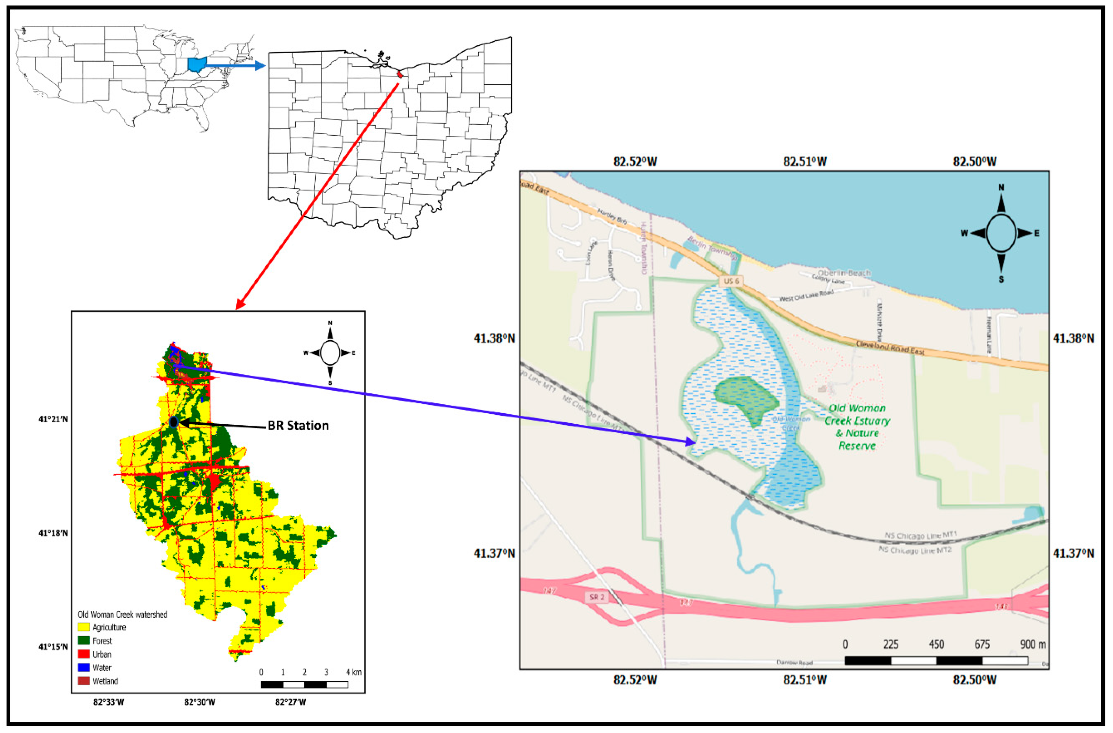
Old Woman Creek (OWC) is a freshwater estuary situated on the southern side of Lake Erie and close to the east of Huron city (Figure 1). The OWC watershed has an elevation range of 173 m to 276 m and covers an area of about 69 km2, with over 60% being used for agriculture and about 25% for forest, which is responsible for the high nutrient inflow to the estuary [12]; the remaining (<15%) consists of urban areas, an estuary, and wetlands. The OWC estuary was designated a National Estuarine Research Reserve (NERR) System in 1980. The OWC National Estuarine Research Reserve (NERR) is located at a latitude of 41°22′34″ N and a longitude of 82°30′42″ W. The estuary dominates the first 3 km in the north of the OWC watershed. It has an area of about 520,000 m2, a mean depth of 0.4 m and an estimated volume of 190,000 m3 at an average water level, with an elevation of 174.1 m IGLD (International Great Lake Datum) 1985 or + 0.6 m LWD (Low Water Datum) [13].
2.2. Data Acquisition
The 10-m resolution Digital Elevation Model (DEM) of Ohio, available at the National Elevation Dataset, was downloaded from Geospatial Data Gateway (https://datagateway.nrcs.usda.gov, accessed on 30 May 2019). The OWC watershed shapefile was extracted using GIS tools from the Ohio state shapefile obtained from the government data catalog (https://catalog.data.gov/dataset/tiger-line-shapefile accessed on 22 August 2018). The shapefile was used to prepare all the GIS layers used for this work.
The 30-m resolution land cover data of Ohio was obtained from the National Land Cover Database (https://www.mrlc.gov/data/type/land-cover, accessed on 30 May 2019) and was processed using GIS tools into five main LULC groups, namely Agriculture, Urban, Forest, Wetland, and Water [14]. Digital Soil data of Ohio were downloaded from the Soil Survey Geographic database (SSURGO) at https://www.nrcs.usda.gov/wps/portal/nrcs/detail/soils/survey accessed on 30 May 2019. from which the study area data were extracted. Stream discharge data were downloaded from the USGS national water information system (https://waterdata.usgs.gov/ accessed on 30 August 2019). The water quality data for calibration and validation were obtained from the water quality lab at Heidelberg University, Tiffin, Ohio. The PRISM climate data of a spatial resolution of 4 km × 4 km from 1981–2017 were downloaded from PRISM Climate Group at http://www.PRISM.oregonstate.edu/ accessed on 30 August 2019. The RCP 8.5 data for the 20 Climate Model Intercomparison Project Phase 5 (CMIP5) ensemble from 1981–2100 were downloaded from the climate data store catalogue (https://climate.copernicus.eu/climate-data-store accessed on 30 Aug 2019) downscaled to a 4 km × 4 km resolution and bias corrected using the distribution-based scaling (DBS) method described by Yang et al. [15]. All GIS layers were prepared with the OWC watershed shapefile. SWAT model version 2012, which runs on ArcSWAT 2012.10.21, was used for this analysis. It was downloaded from Texas A & M University website (https://swat.tamu.edu accessed on 30 May 2019).
2.3. Description of the SWAT Model
The Soil and Water Assessment Tool (SWAT), an improved version of the Simulator for Water in Rural Basins (SWRRB), is a watershed scale model, developed by Jeff Arnold for the United States Department of Agriculture—Agricultural Research Services (USDA-ARS) to assess the impact of environmental management and pollution within watersheds on water quality [16]. It was specifically designed to forecast the influence of land management on water quality, sediment, and nutrients yields in large river basins with changing land use/land cover, soil condition, and management practices over a long-time interval [16]. SWAT is a physically based, continuous, and multitasking model. It is computationally structured and very productive, with the capability of simulating a daily time resolution using temporal, spatial, and meteorological information. Arnold et al. [5] presented a full description of SWAT’s integral parts, which include weather, crop growth, pesticide, hydrology, management practices, soil types and temperature, channel and reservoir routing, and sediment and nutrient transports. In SWAT hydrological modeling, the whole basin is segmented into separate sub-basins, which are then divided into different hydrological units [17]. The hydrological response unit (HRU) is the smallest component in a sub-basin of the hydrological model, which consists of land use, soil types, and slope defined by the modeler [18]. SWAT does not provide for spatial data input for modeling, and hence, ArcSWAT was introduced, which is the graphical interface connecting the SWAT model and ArcGIS that adds spatial data, such as digital stream network, land use/land cover, agricultural management practices, soil, and weather, and assigns simulation intervals [19].
2.4. Hydrological Model Setup
The OWC hydrological model was set up and parameterized in the ArcSWAT 2012 interface. The prepared Digital Elevation Model (DEM) and digital stream dataset were loaded into SWAT model for watershed delineation, drainage, and slope analysis. The stream network was superimposed and established on the DEM, the minimum drainage area threshold method was first used to automatically generate the sub-basin outlets, after which an outlet was created at the Berlin station, where we have observed data for calibration and validation. The OWC watershed was finally delineated with a size of 66.95 km2 and a total of 103 sub-basins. In the HRU definition, three classes of slope, namely, 0–3% for flat, 3–15% for medium, and >15% for steep, were created for the watershed using the DEM data with soil and land use data added to establish the hydrological parameters of the sub-basins. A threshold value of 10% was used to remove small land use, soil, and slope from the model set up. Classes of land use, soil, and slope which occupy an area <10% of the sub-basin were redistributed on the major ones so that minor classes were removed, and modeling was done on 100% of the area of the sub-basin. This approach yielded a total of 12 land use classes that include open waters, developed open space, developed low intensity, developed medium intensity, developed high intensity, barren land, deciduous forest, evergreen forest, herbaceous, hay, cultivated crops and woody wetlands, and 81 soil classes based on the SSURGO soil classification. Land use, soil, and slope were reclassified and overlain for complete definition and a total of 479 HRUs were created.
Weather stations and prepared climate data in the form of minimum, maximum, and daily average for precipitation and temperature were added. Other weather data, such as relative humidity, solar radiation, and wind speed, were generated in SWAT.
2.5. Crop Rotation
The main crop types planted at the OWC watershed with the best management practices described by Confesor et al. [20] and Scavia et al. [12] were replicated in the SWAT hydrological model set up for the water quality modeling. The crop cover GIS layer for 2015–2017 was used to establish a three-year crop rotation plan for each of the 479 HRU in the OWC watershed. The main crop types planted are corn, soybean, and wheat with the following management practices:
- Corn Crop: Soil chisel, plowing, and fertilizer application, nitrogen-phosphorus-potassium (11-52-00, 130 kg/ha) were done in fall. The model was programmed to retain 20% of the fertilizer on the surface. Anhydrous ammonia (100 kg/ha) was applied two times in the spring; the first was done prior to seeding and the second was done at one month after seeding. Corn harvesting was done in the fall at about five months after seeding.
- Soybean crop: SWAT was programmed for no-till and fertilizer (11-52-00, 95 kg/ha) application before seeding at 100% at the soil surface in the spring. Harvesting was done in the fall five months after the completion of seeding.
- Wheat crop: SWAT was programmed for no-till and fertilizer (18-46-00, 130 kg/ha) application was done before seeding at 100% at the soil surface in the fall. In the early spring, fertilizer broadcast (11-52-00,150 kg/ha) was repeated, and harvesting was done in July.
2.6. Sensitivity Analysis
A sensitivity analysis was performed to ascertain the relative importance of each of the parameters in the SWAT hydrological model and to select the best parameters for calibration as recommended in the SWAT’s user manual [16]. The knowledge obtained from the literature review of SWAT sensitivity and calibration [21,22] was used to test parameters in the sensitivity analysis and a total of 56 parameters were finally selected for optimization (Table 1). The selected parameters were tested using the “one-factor-at-a-time” (OAT) principle as recorded in Van Griensven et al. [22]. This involves changing the value of each parameter one at a time and calculating the objective functions with the assumption that the observed changes in the output of each simulation run is due to the changes made on the values of each parameter. The objective function was calculated as the root mean square error (RMSE) of the observed and the simulated output for flow, sediments, SRP, total phosphorus, and total nitrogen. Given the parameters α with total number n and the model of interest y (α), the sensitivity to a perturbation ∆ of the ith parameter is given as:
The basic statistics of each parameter including the minimum, 25th percentile, mean, 75th percentile, and the maximum were computed and used in making the first set of simulations. For the second stage of simulations, each parameter’s minimum and maximum limit was stipulated, and simulations were run with each parameter changing four times with five basic statistical values of the remaining parameters. For example: simulations were made with the minimum of parameter “x” and each of the 25th percentile, mean, 75th percentile, and maximum of the remaining parameters; then, the 25th percentile of “x” was run with each of the minimum, mean, 75th percentile, and maximum of the remaining parameters and this was done for all the 56 parameters. A total of 1120 simulations (4 parameters × 5 basic statistical parameters × 56 + 5 first set of simulations) were made.
2.7. Calibration and Validation
The curve number for each HRU was separately calibrated giving a total of 479 curve numbers. The soil evaporation compensation factor was calibrated for each land use category. Calibration was done by modifying the autocalibration method developed by Confesor and Whittaker [23] and a total of 56 parameters were selected for optimization in the calibration process. The hydrologic characteristics of the watershed were thoroughly considered to stipulate the range of the selected calibration parameters for optimum results. The calibrated and validated variables are streamflow, sediment (TSS), organic nitrogen, mineral nitrogen, organic phosphorus (SRP), total nitrogen, and total phosphorus. The streamflow data were obtained from the USGS gage station at Berlin Road in the OWC watershed, while the water quality data were obtained from the water quality laboratory at the Heidelberg University, Tiffin, Ohio. The remaining three water quality variables included in the simulation (chlorophyll a, CBOD, and dissolved oxygen) were not calibrated as daily data were not available for calibration; it is noted that this may impact the result of the simulations for these three variables. The most complete daily streamflow data obtained at US gage station at Berlin station were from 2015–2017; hence, the calibration period was set from 5 May 2015 to 31 December 2016 (607 observations) and validation was from 1 January 2017 to 31 December 2017 (365 observations), and a warm-up period of three years was used for all simulations.
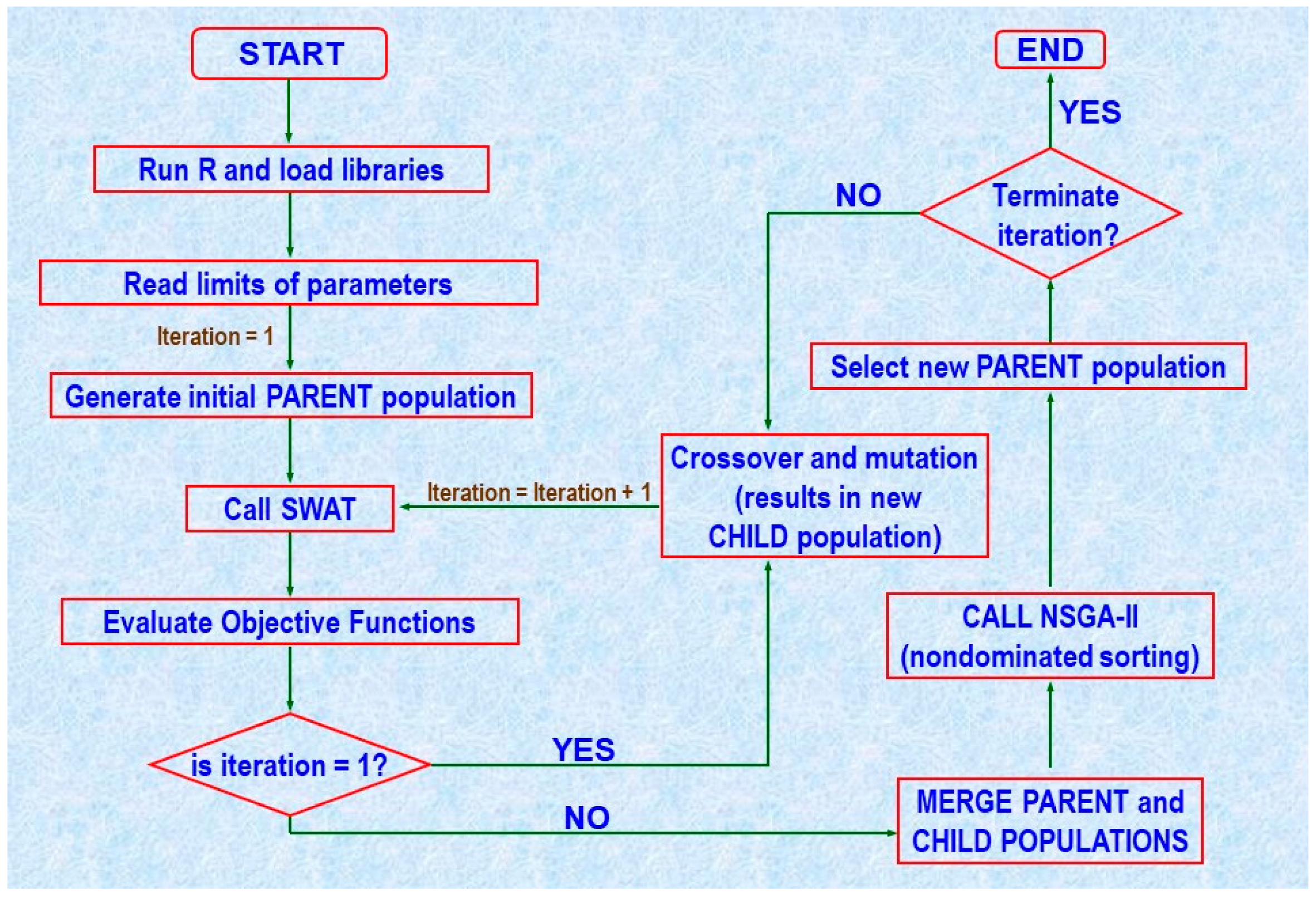
The computational algorithm for optimization was executed on an IBM server with two quad-core processors. Fortran was originally used to create SWAT and the multi-objective evolutionary algorithm (the nondominated-sorting genetic algorithm, NSGA) [24] as libraries compatible with R. The genetic algorithm package (genalg) of the R statistical language [25] was used to execute the NSGA (Figure 2). Five objective functions were used to evaluate the parent and child population in the first iteration performed and SWAT’s source code was modified and used as a subroutine for each of the solutions in the subsequent evaluation steps [24].
2.8. Evaluation Criteria
The purpose of the objective functions (flow, TSS, SRP, total p, and total n) is to minimize the average root mean square error (RMSE) of the observed versus simulated values. The RMSE equation is given as:
The performance of the calibrated SWAT model was evaluated by comparing the simulated with the observed variables of the 10 variables of interest in the calibration and validation stage using three statistical indices: Percentage bias/percentage error (PBIAS (%)), Nash–Sutcliffe model efficiency (NSE) [23], and Coefficient of R2:
where QSm and QOb are the simulated and the observed (measured) daily streamflow, respectively, at a given time i and n represents the total number of days for the period of simulation.
Nash–Sutcliffe model efficiency [26] ranges from negative infinity to 1, with the latter indicating a perfect match between the observed and simulated.
2.9. Simulation with Varying Agricultural Percentages
To evaluate the effect of watershed agricultural land use on flow and water quality variables, four simulation scenarios consisting of varying percentages of agricultural land use (20%, 40%, 53.5%, and 80%) were created and added to the baseline calibration scenario (65.2%). The scenarios’ percentages were created by converting agriculture to forestry for lower percentages and forestry to agriculture for higher percentage while keeping urbanization, wetland, and water constant. The values for the percentages were hypothetical, chosen to simulate the progressive effect of agriculture on water quality. A warm-up period of three years (2012–2014) was used for all the simulations. All simulations were run annually from 2015–2017. One annual simulation with PRISM data and 20 annual simulations with CMIP5 models were run for each of the scenarios for the period of 2015–2017. In total, 105 simulations, one for each scenario of the PRISM climate data and 20 for each scenario with CMIP5 models, were performed. For each of the CMIP5 scenarios, the 20 model results were averaged to remove inter-model variability and the results were averaged across the years to eliminate inter-annual variability.
3. Results
3.1. Calibration and Validation
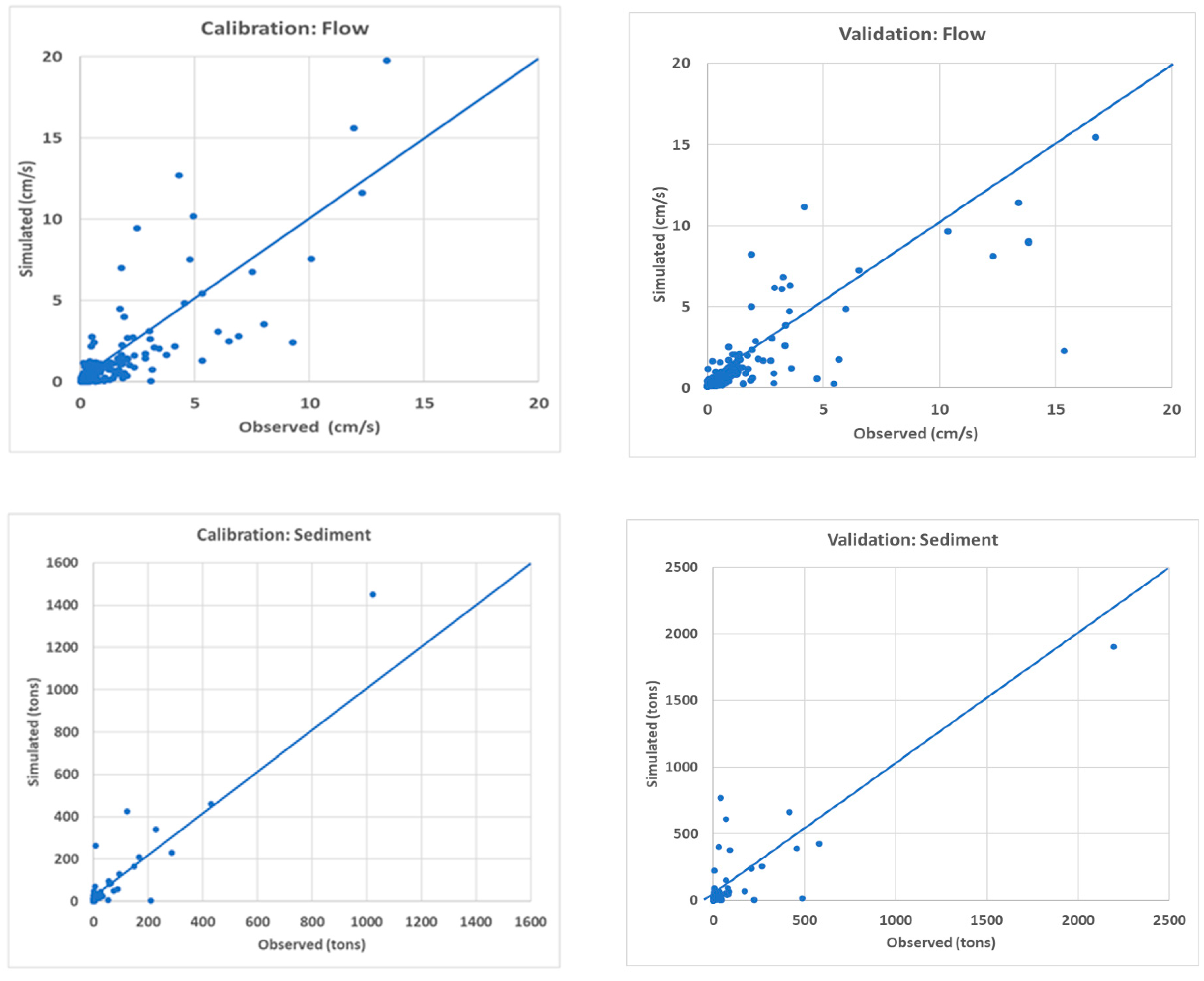
The calibrated hydrological model of the Old Woman Creek watershed simulated the daily streamflow and the water quality variables for a period of 1 year and 7 months (5 May 2015–31 December 2017) with a Nash–Sutcliffe efficiency of 0.60 and an R2 value of 0.69. The validation run was for 1 year (January–December 2017) and gave a Nash–Sutcliffe efficiency of 0.7 and an R2 value of 0.7. The evaluation criteria for the calibration and validation results for flow and water quality variables are shown in Table 1 and Table 2. The 1:1-line plots for calibration and validation results for the observed and simulated variables are shown in Appendix A. PBIAS for calibration and validation were 5.7% and 11.8%, respectively, for flow, showing slight under-prediction (Table 1 and Table 2). The positive values indicate under-prediction in the simulation and negative values indicate over-prediction in the simulation. This means that the simulations made with this model will underestimate flow and overestimate water quality variables by their respective PBIAS values. The calibrated model was able to accurately pick the high flow events with slight underestimation. Substantial differences between the measured and the simulated streamflow peak events, after optimization of parameters controlling the release of runoff into the main streamflow channel, were reported by previous studies [17,27]. This uncertainty might have occurred either when preference was given to the major soils and land covers of the HRUs or the soil properties were not properly assigned to the hydrological soil group studies, but the uncertainty has been minimized by the use of detailed soil data (SSURGO) [16,27]. The use of RMSE as an objective function in automatic calibration has been reported by Boyle’s et al. [28] to yield a biased simulation. The underestimation might be due to the high sensitivity of the optimized model to peak flow events due to the use of RMSE as the objective function, because it squares the difference between the measured and the simulated streamflow [18].
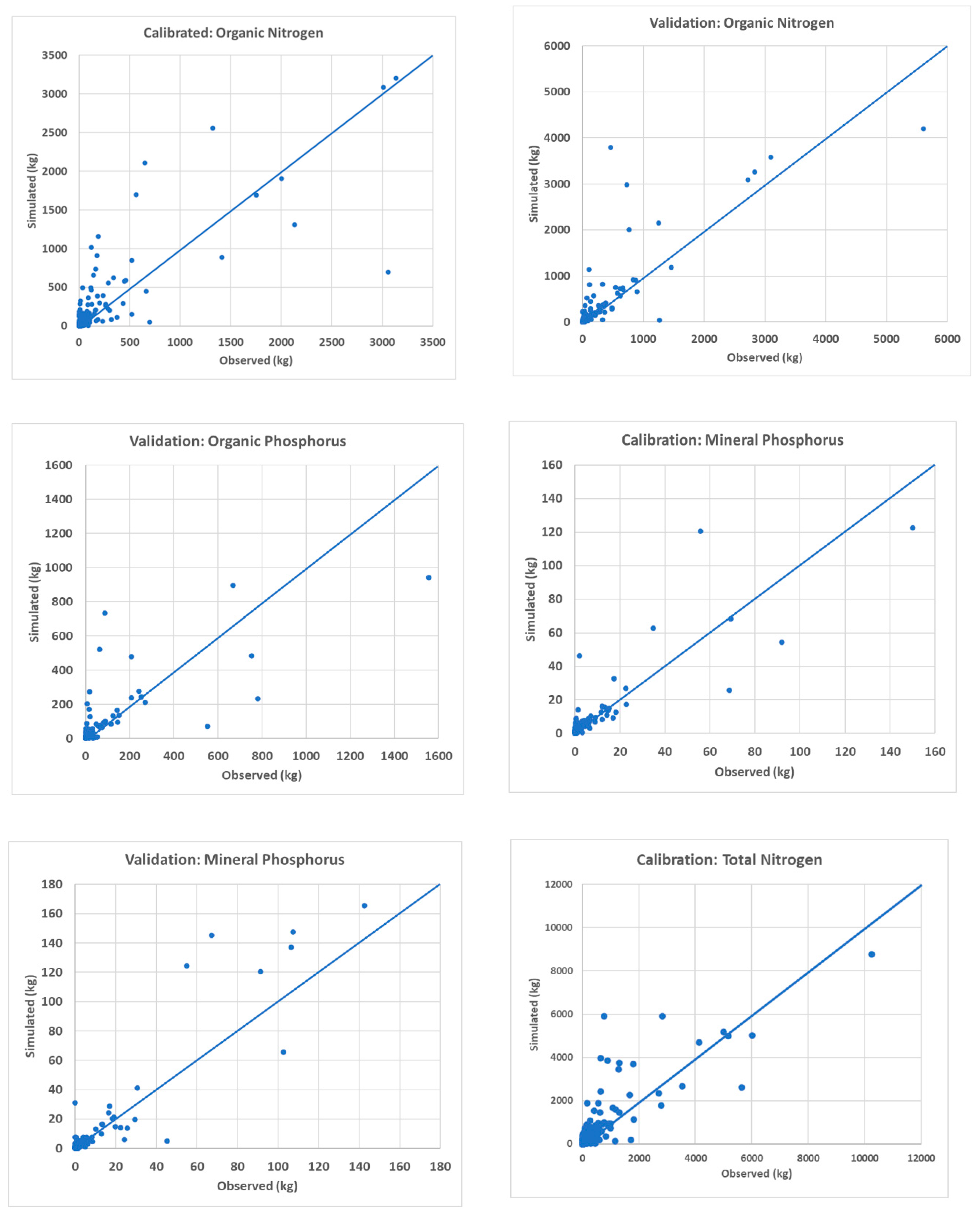
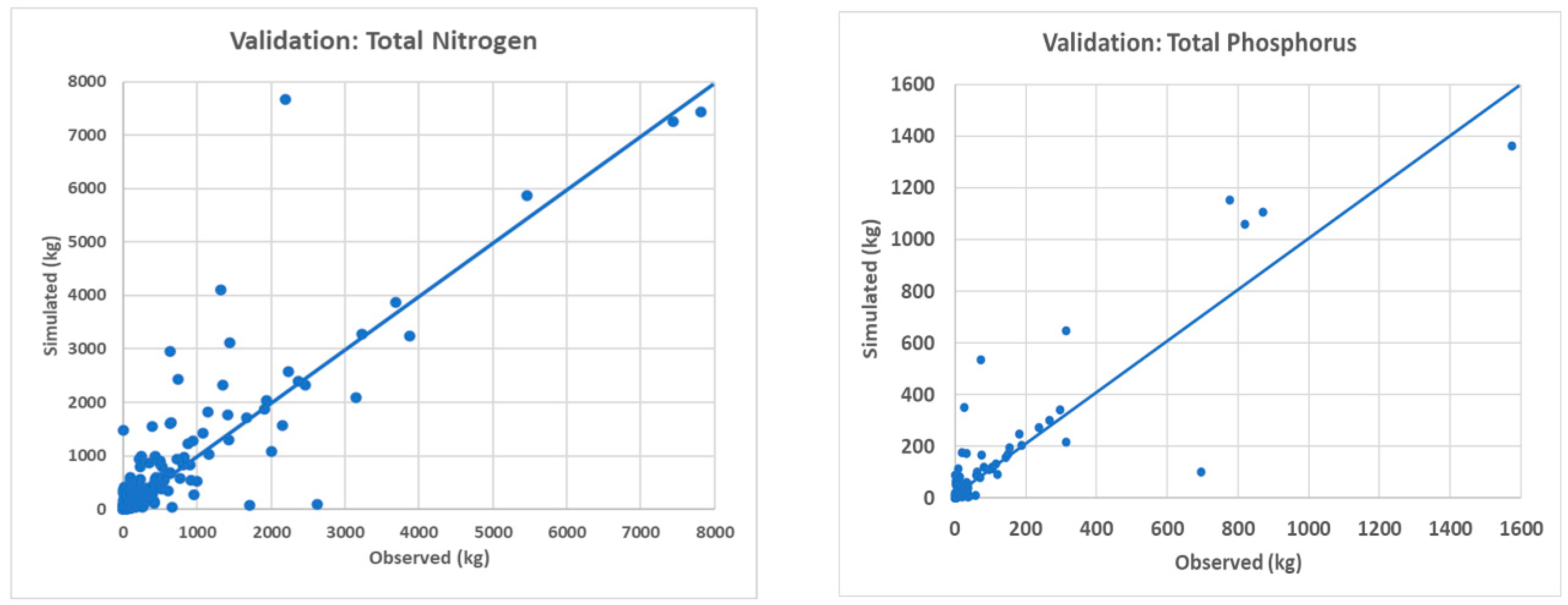
The results of sediment calibration and validation showed good correlation with the calibration, which has an NSE value of 0.7 and an R2 value of 0.9, and validation, which has an NSE value of 0.7 and an R2 value of 0.8 (Table 1 and Table 2). The sediment transport was largely overestimated with the calibration and validation PBIAS values of −40.45 and −32.58. The peak sediment transport events correspond to the peak streamflow events (Appendix A), which indicates that the streamflow controls sediment transport. Other variables, including organic nitrogen, organic phosphorus, mineral phosphorus, total phosphorus, and total nitrogen, were slightly overestimated as shown by the calibration and validation results (Table 2 and Table 3).
3.2. Simulation Results
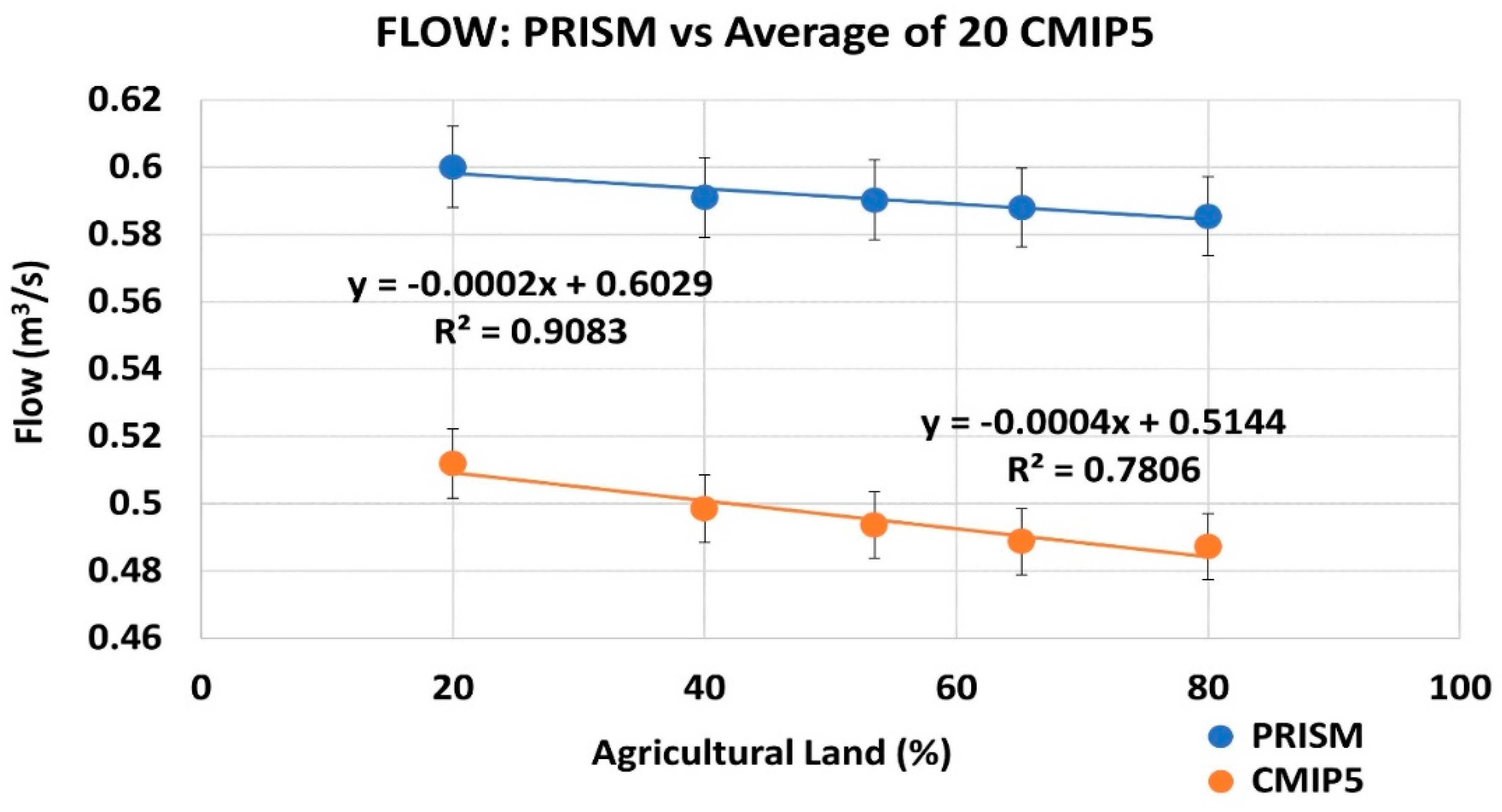
The result of the 105 simulations run with varying percentages of agricultural land use using PRISM and CMIP5 climate data are shown in Figure 3, Figure 4, Figure 5, Figure 6, Figure 7, Figure 8, Figure 9, Figure 10 and Figure 11. The error bars show the degree of variability in each result as they were constructed from the standard deviation of the result. The variability between the PRISM and CMIP5 result is statistically insignificant when the vertical error bars overlap and statistically significant when the vertical error bars do not overlap. For all the variables of interest, the average of the simulation results from the 20 GCMS is consistent with the results from PRISM [29,30].
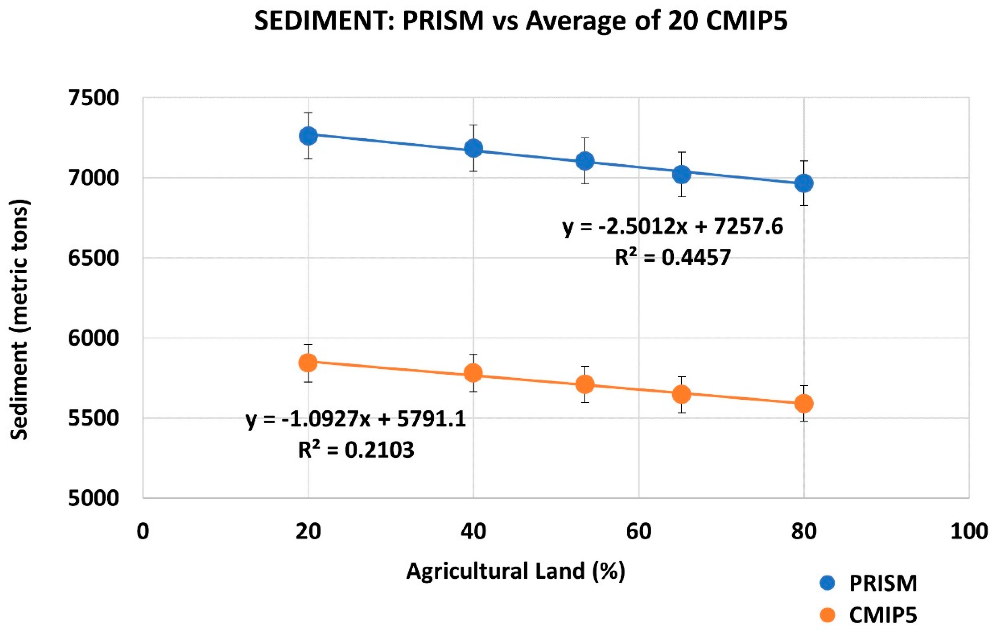
Both PRISM and CMIP5 flow results show a strong negative correlation with changes in the percentage of agricultural land use with a slope of −0.0002 m3 s per percent of agricultural land and an R2 value of 0.9 for PRISM and a slope of −0.000004 m3 s per percent of agricultural land and an R2 value of 0.8 for CMIP5. CMIP5 results significantly underestimated flow because CMIP5 precipitation values for this period are slightly lower than PRISM values. Both results of PRISM and CMIP5 sediment simulation show a weak negative correlation with the percentages of agricultural land, with PRISM having a slope of −2.5 metric tons per percent of agricultural land and an R2 value of 0.5 and CMIP5 having a slope of −1.1 metric tons per percent of agricultural land and an R2 value of 0.2. CMIP5 results largely underestimated sediment, similar to the flow result.
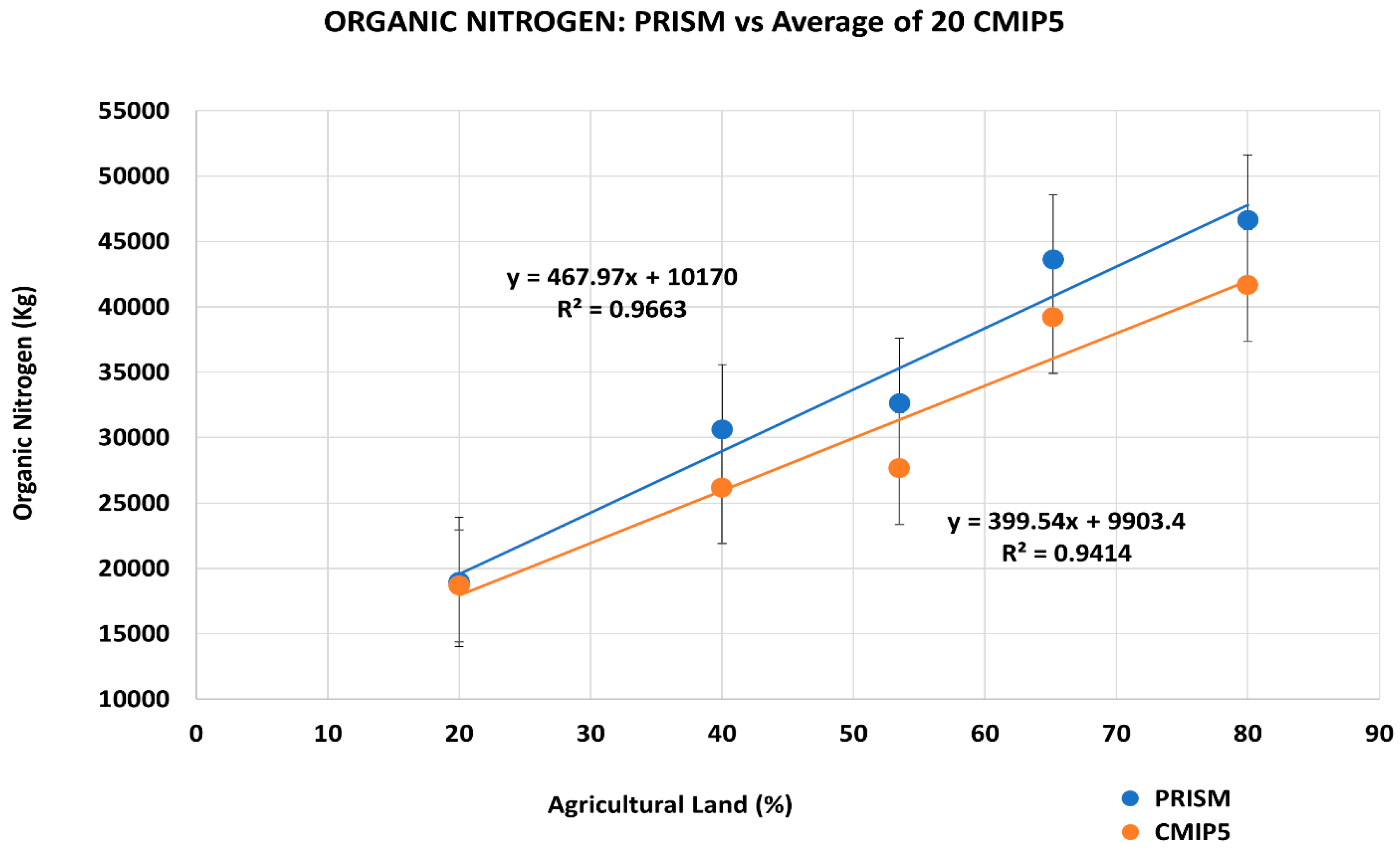
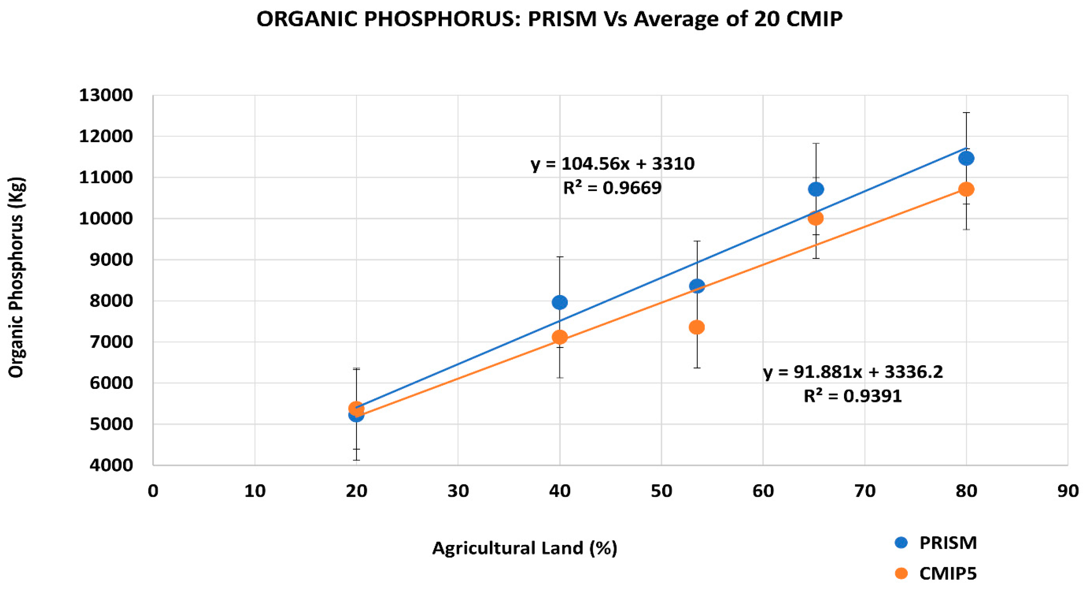
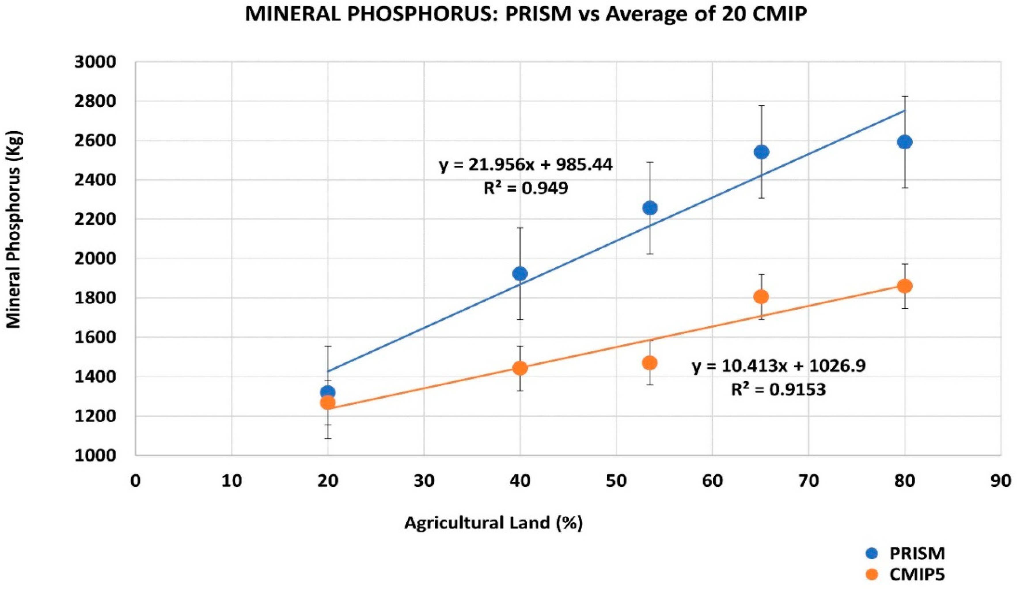
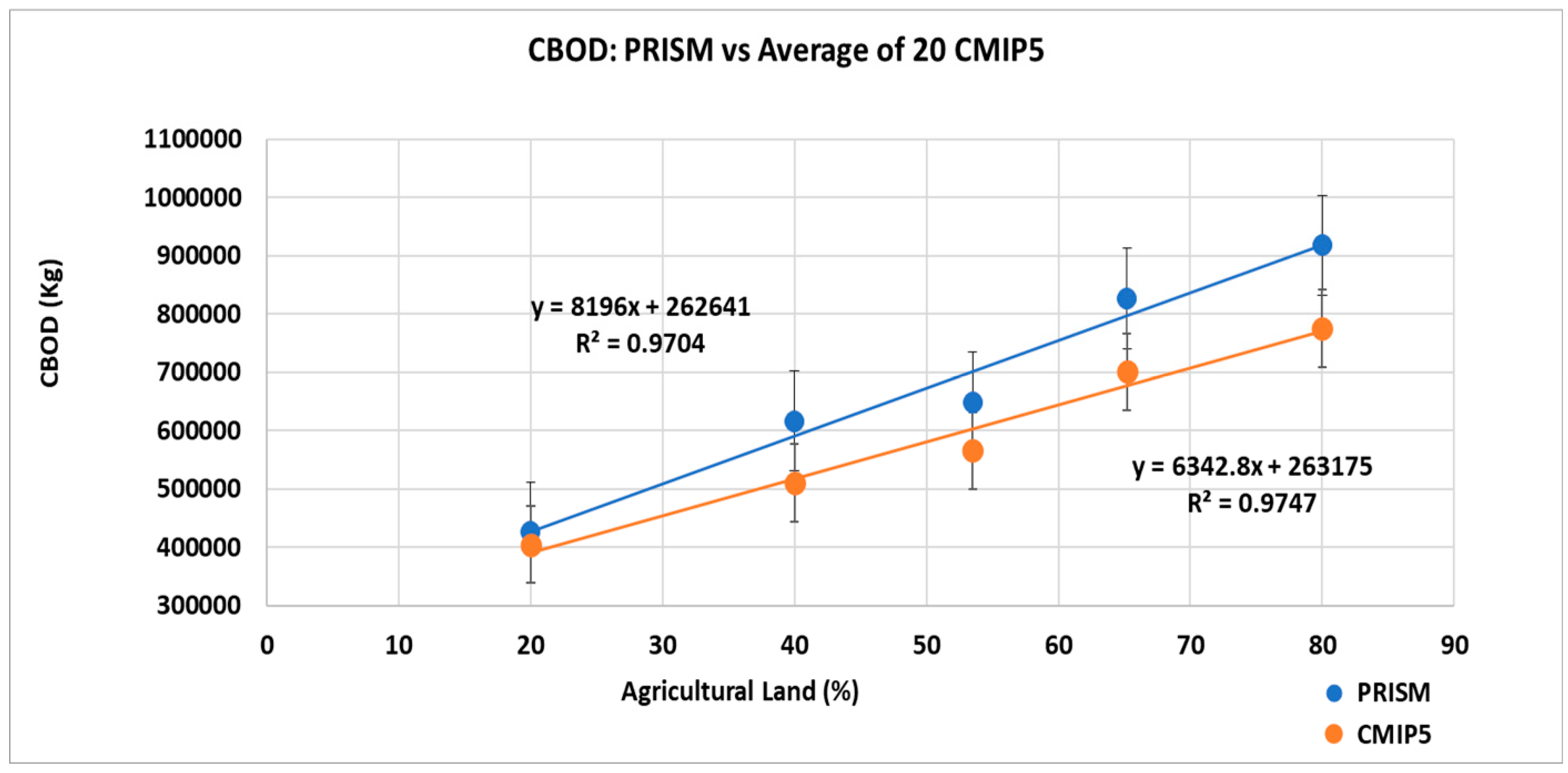
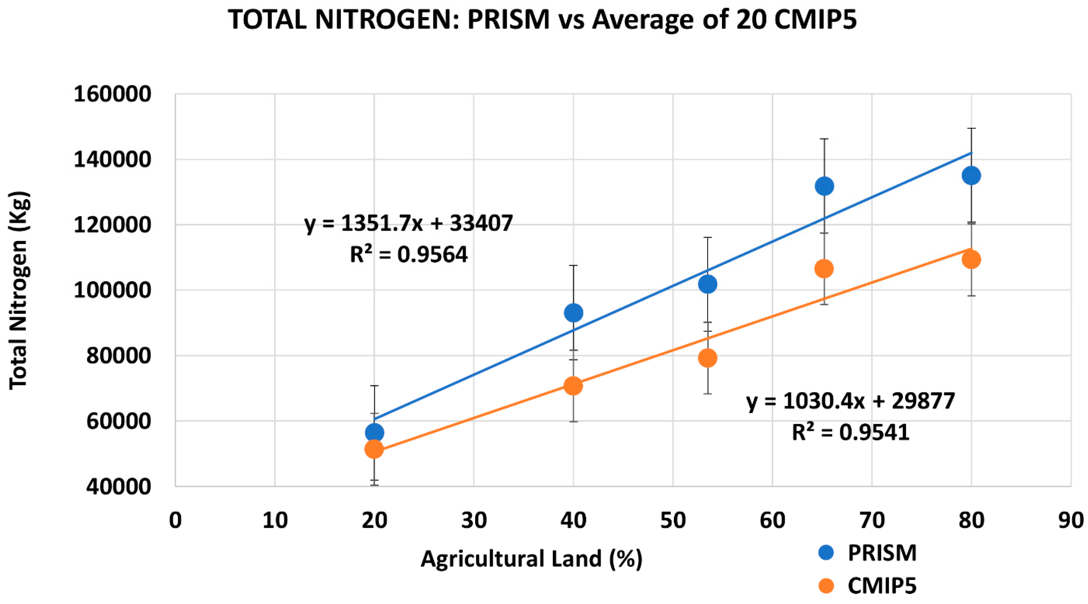
The results of the simulations for the five nutrients under consideration with PRISM data and the CMIP5 model show a strong positive correlation between the nutrients and agricultural land use. Organic nitrogen in the PRISM and CMIP5 results have similar slope values of 4.680 kg per percent of agricultural land and 399.5 kg per percent of agricultural land and R2 values of 0.97 and 0.94, respectively. The slight underestimation observed in the CMIP5 results of organic nitrogen is statistically insignificant, which shows a good agreement between the PRISM results and the average of the 20 CMIP5 results for the OWC watershed. The results of the PRISM and CMIP5 simulations for organic phosphorus show a close resemblance with the slope values of 104.6 kg per percent of agricultural land and 91.9 kg per percent of agricultural land and R2 values of 0.97 and 0.94, respectively. Underestimation in organic phosphorus recorded in CMIP5 results relative to PRISM result was statistically insignificant. The result of the simulation of mineral phosphorus was slightly different, with PRISM and CMIP5 results having slopes of 22.0 kg per percent of agricultural land and 10.4 kg per percent of agricultural land and R2 values of 0.95 and 0.92, respectively. While there was a good correlation between the two results, CMIP5 results largely underestimated mineral phosphorus with respect to the PRISM results and the underestimation was statistically significant. For chlorophyll a simulation, the slopes of 7.7 kg per percent of agricultural land was obtained for the PRISM results and 6.7 kg per percent of agricultural land for the CMIP5 results, with an R2 value of 0.97 in both cases. A similar trend was observed in the CBOD simulation results, with PRISM results having a slope of 8196 kg per percent of agricultural land and an R2 value of 0.97, and CMIP5 results having a slope of 6342.8 kg per percent of agricultural land and an R2 value of 0.97. The slopes for PRISM and CMIP5 simulation results for total nitrogen were 1351.7 kg per percent of agricultural land and 1030.4 kg per percent of agricultural land and the R2 values were 0.96 and 0.95, respectively, which shows good agreement and statistically insignificant underestimation with respect to the CMIP5 results. The simulation results for total phosphorus also show good correlation, with PRISM and CMIP5 having similar slopes of 126.5 kg per percent of agricultural land and 102.3 kg per percent of agricultural land and R2 values of 0.97 and 0.94, respectively, and statistically insignificant underestimation was recorded in CMIP5 results.
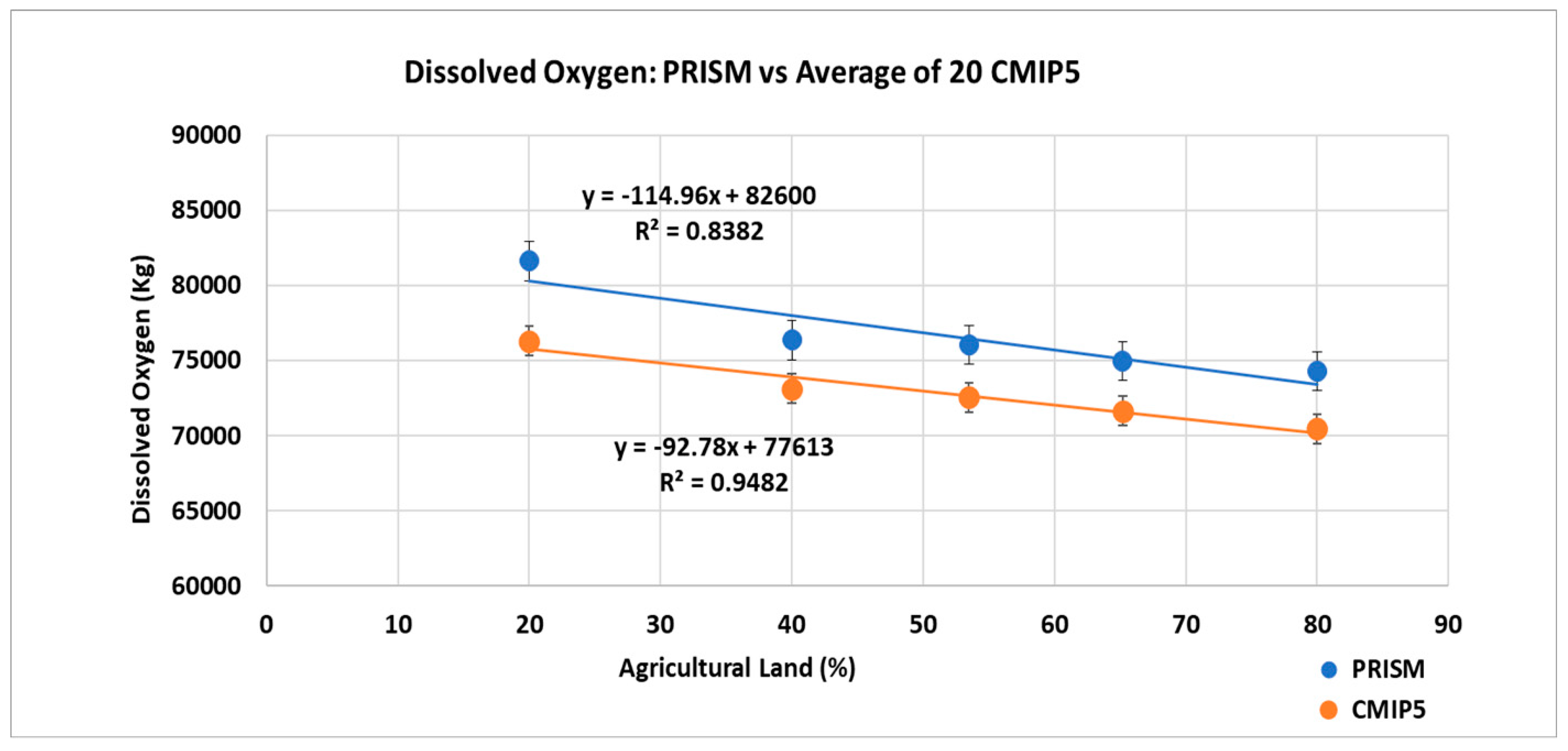
A negative correlation was observed between dissolved oxygen and agricultural land in both PRISM and CMIP5 simulation results. A slope of −115 kg per percent of agricultural land and an R2 value of 0.84 was observed in the PRISM results, while a slope of −92.8 kg per percent of agricultural land and an R2 value of 0.95 was observed in the CMIP5 results.
Table 4
shows the percentage of change in the simulated variables for both the PRISM result and the average of the 20 different CMIP5 model results relative to the 20% agricultural scenario. The 65.2% agricultural percentage represents the current condition. A comparatively low decrease rate was observed in flow, sediment, and dissolved oxygen, while a high increase rate was observed in other variables. The most probable change is a slight increase or decrease in the percentage of agricultural land from the present condition, which are the 80% and the 53.5% agricultural scenarios. An increase in the percentage of agricultural land from the current (65.2%) to 80% would decrease flow by 0.4% in PRISM results and 0.3% in the CMIP5 results and would decrease sediment by 0.8% in the PRISM results and 0.9% in the CMIP5 simulation. The same increase from the current condition to 80% in agricultural land will increase chlorophyll a by 21.3% in the PRISM results and 20% in the CMIP5 results and will increase total nitrogen by 5.8% in the PRISM results and 5.4% in the CMIP5 results.
4. Discussion
The weak negative correlation observed between the percentages of agricultural land and flow for both PRISM and CMIP5 results shows that an increase in agricultural land in the OWC watershed will reduce the streamflow. This is because the increase in agricultural land will increase the surface area available for infiltration, which reduces the contribution to runoff from the agricultural land, thereby reducing the streamflow. Similarly, because the stream flow is laden with the suspended sediment, a high energy flow would transport more sediment, while low energy flow would transport less sediment; a reduction in the streamflow would lead to the reduction in the sediment transport, and this accounts for the similarity observed in the plots for the PRISM and the CMIP5 flow and sediment. The overall sediment effect is due to the changes in streamflow, changes in loadings to the stream, and the model uncertainty.
The strong positive correlation observed between the agricultural land and organic nitrogen transport shows that with more land being used for agricultural purposes within the OWC watershed, there will be more organic nitrogen transport into the OWC estuary, which would affect the estuarine water quality. The organic nitrogen sources could be traced to the fertilizer application for soil improvement and crop yield. The strong positive correlation observed between organic phosphorus and agricultural land shows that with more land being used for agricultural purposes, there would be an increase in the quantity of organic phosphorus transported from the farmland to the estuary, which would affect the estuarine water quality.
This same is also true for mineral phosphorus. The excess nitrogen and phosphorus being added to the estuary with increase in agriculture land, would raise nutrient content of the estuary, which would be observed as an increase in the total nitrogen and total phosphorus content. The increase in the total nutrient content in the estuary will impact the estuary water quality, which could have a negative impact on the estuary ecosystem.
The decrease in the dissolved oxygen level with increasing agricultural land indicates a degradation in water quality with increasing agricultural land. The progressive decrease in the oxygen level would lead to hypoxia or anoxia, which would affect the life-supporting capability of the aquatic environment. When the oxygen level in the water drops below the threshold for certain aquatic animals, they may die or exit to other places. Drastic changes in the aquatic life would affect the aquatic ecosystem. Changes in the ecosystem would have economic implications on the estuary and agricultural productivity within the watershed. With an increasing percentage of agricultural land, agricultural productivity increased with a higher influx of nutrients into the estuary, which may lead to an increase in the cost of water purification. The 4x4km climate data was adequate for the simulation runs given the small area of the watershed.
Similar work was done by Rocha et al. [31], who employed a different yield/exportation ratio for both the rate and the method of application of the nitrogen fertilizer to evaluate the affordable agricultural practices capable of supporting the water quality improvement.
Linter, A.M., and Weersink, A. [32] studied the effects of 15 different management practices on sediment transport and phosphorus enrichment in the Lake St. Clair drainage basin sub-watershed in Canada using different three-year crop rotation plans for corn (C), soya (S), and wheat (W). They estimated the runoff, infiltration, and three-year average profits for each of the management practices, and found that the three-year rotation plan with CSS produced the greatest profit. Mastrorilli et al. [33] applied the methodology they developed for estimating the economic and technical worth of the hydrological benefits of the ecosystems to a watershed in the Bonis basin in Calabria, Italy. They estimated the economic value of four hydrological benefits under four land use scenarios and established that the methodology permits a quantitative evaluation of the impact of land use on water resource and an economic guide for watershed land use management.
The limitation of this work is that the values of the simulation results for the three water quality variables that were not calibrated due to data availability (chlorophyll a, CBOD, and dissolved oxygen) may be slightly impacted.
Further simulations may attempt to see the effect of each of the three main crops (corn, soy, and wheat) planted in the watershed or the effect of a combination of any two of the crops on water quality. This can be done with scenarios simulations by converting the entire agricultural land into corn, converting the entire agricultural land into soy, and converting the entire agricultural land into wheat. Other simulation scenarios may be created by converting the entire agricultural land into any two of the three crops, which can be done in three ways, consisting of corn and soy, corn and wheat, and soy and wheat. Thus, a total of six different simulation scenarios can be created, and the effect of each scenario can be evaluated. Additional simulation scenarios can also be created using different management practices and fertilizer application methods, and the percentage change in flow and water quality variables can be evaluated.
5. Conclusions
The average of the 20 CMIP5 results for the OWC estuary is consistent with PRISM results. This implies that the 20 CMIP5 models are suitable for the future water quality simulations for the OWC watershed. CMIP5 underestimated flow and sediment in the same pattern, which implies that the flow controls the sediment transport. CMIP5 slightly underestimated most of the nutrients, including organic nitrogen, organic phosphorus (particulate p), total nitrogen, and total phosphorus, and largely underestimated mineral phosphorus (soluble reactive p) relative to PRISM results. A large increase in agricultural land use brings about a small decrease in flow and sediment transport, which shows that an increase in agricultural land would increase the surface area available for infiltration, reduce surface runoff contribution from the agricultural land, and eventually reduce the streamflow. A low energy streamflow would carry less suspended sediment. Conversely, an increase in agricultural land would lead to an increase in the transport of all nutrients. This is because an increase in agricultural land is associated with an increase in fertilizer applications for corn, soya, and wheat planted in the OWC watershed, which increases the concentration of nutrients in the streamflow. An increase in nutrients would drive eutrophication, which would lead to a high CBOD and low dissolved oxygen level, causing water quality deterioration. Poor water quality would impact the aquatic life, causing an imbalance in the ecosystem, which would affect the use of the estuary for its various purposes. As is indicated by the progressive decrease in the dissolved oxygen level with the increase in agricultural land, and the progressive increase in total nitrogen and total phosphorus, it is recommended that the percentage of the agricultural land in the OWC watershed not is increased beyond the current level. Management should employ best management practices (BMPs) in farming operations depending on the use of the agricultural land.
Author Contributions
Conceptualization, J.D.O., I.A.O. and R.B.C.J.; methodology and software, R.B.C.J. and J.D.O.; validation, J.D.O. and R.B.C.J.; formal analysis, visualization, and writing—original draft preparation, J.D.O.; project supervision, I.A.O. and R.B.C.J.; writing—review and editing, I.A.O. and R.B.S.J. All authors have read and agreed to the published version of the manuscript.
Funding
This research received no external funding but the first author was partially supported by a graduate stipend from the Department of Geology, Kent State University, Ohio, USA.
Institutional Review Board Statement
Not applicable.
Informed Consent Statement
Not applicable.
Data Availability Statement
Not applicable.
Acknowledgments
The authors wish to acknowledge the participation of Abdul Shakoor and Anne Jefferson of the Kent State University, Ohio in the review of the original dissertation format of this manuscript. We would also like to acknowledge the support received from the Old Woman Creek National Estuarine Research Reserve, Ohio, USA for data accessibility, the National Water Quality Laboratory at Heidelberg University, Ohio, USA for access to their Beowulf cluster of computers, the Department of Geology Kent State University, Ohio, USA, and the Texas Institute for Applied Environmental Research (TIAER), Tarleton State University, Member of the Texas A&M System, Stephenville, Texas, USA.
Conflicts of Interest
The authors declare no conflict of interest.
Appendix A
Figure A1.
1:1-line Plots for Calibration and Validation results for the observed and simulated variables.
Figure A1.
1:1-line Plots for Calibration and Validation results for the observed and simulated variables.


References
- Nazari-Sharabian, M.; Taheriyoun, M.; Ahmad, S.; Karakouzian, M.; Ahmadi, A. Water quality modeling of Mahabad Dam watershed–reservoir system under climate change conditions, using SWAT and system dynamics. Water 2019, 11, 394. [Google Scholar] [CrossRef] [Green Version]
- Bhuyan, S.J.; Marzen, L.J.; Koelliker, J.K.; Harrington, J.A.; Barnes, P.L. Assessment of Runoff and Sediment Yield Using Remote Sensing, GIS and AGNPS. J. Soil Water Conserv. 2002, 57, 351–364. [Google Scholar]
- Bhattarai, G.; Hite, D.; Hatch, U. Estimating the impact on water quality under alternate land use Scenarios: A watershed level BASINS-SWAT modeling in West Georgia, United States. In Efficient Decision Support Systems: Practice and Challenges in Multidisciplinary Domains; Jao, C., Ed.; IntechOpen: London, UK, 2011. [Google Scholar]
- Haverkamp, S.; Fohrer, N.; Frede, H.G. Assessment of the effect of land-use patterns on hydrologic landscape functions: A comprehensive GIS-based tool to minimize model uncertainty resulting from spatial aggregation. Hydro Process. 2005, 19, 715–727. [Google Scholar] [CrossRef]
- Arnold, J.G.; Srinivasan, R.; Muttiah, R.S.; Williams, J.R. Large area hy-drologic modeling and assessment—Part 1: Model development. J. Am. Water Resource Assoc. 1998, 34, 73–89. [Google Scholar] [CrossRef]
- Holtan, H.N.; Lopez, N.C. USDAHL-70 Model of Watershed Hydrology; Techical Bulletin No. 1435; United States Department of Agriculture: Washington, DC, USA; pp. 1–84.
- Lahlou, M.; Shoemaker, L.; Choudhury, S.; Elmer, R.; Hu, A. Better Assessment Science Integrating Point and Nonpoint Sources (BASINS); version 2.0; User’s Manual (No. PB-99-121295/XAB); Tetra Tech, Inc.: Fairfax, VA, USA; EarthInfo, Inc.: Boulder, CO, USA; Environmental Protection Agency, Standards and Applied Science Division: Washington, DC, USA, 1998.
- Woznicki, S.A.; Nejadhashemi, A.P. Sensitivity Analysis of Best Management Practices Under Climate Change Scenarios1. J. Am. Water Resour. Assoc. 2011, 48, 90–112. [Google Scholar] [CrossRef]
- Michalak, A.M.; Anderson, E.J.; Beletsky, D.; Boland, S.; Bosch, N.S.; Bridgeman, T.B.; Chaffin, J.D.; Cho, K.; Confesor, R.; Daloğlu, I.; et al. Record-setting algal bloom in Lake Erie caused by agricultural and meteorological trends consistent with expected future conditions. Proc. Natl. Acad. Sci. USA 2013, 110, 6448–6452. [Google Scholar] [CrossRef] [PubMed] [Green Version]
- Khanna, M.; Yang, W.; Farnsworth, R.; Önal, H. Cost-Effective Targeting of Land Retirement to Improve Water Quality with Endogenous Sediment Deposition Coefficients. Am. J. Agric. Econ. 2003, 85, 538–553. [Google Scholar] [CrossRef]
- Du, F.-H.; Tao, L.; Chen, X.-M.; Yao, H.-X. Runoff Simulation Using SWAT Model in the Middle Reaches of the Dagu River Basin. In Sustainable Development of Water Resources and Hydraulic Engineering in China; Dong, W., Lian, Y., Zhang, Y., Eds.; Springer: Cham, Switzerland, 2019. [Google Scholar]
- Scavia, D.; Kalcic, M.; Muenich, R.L.; Read, J.; Aloysius, N.; Bertani, I.; Boles, C.; Confesor, J.; DePinto, J.; Gildow, M.; et al. Multiple models guide strategies for agricultural nutrient reductions. Front. Ecol. Environ. 2017, 15, 126–132. [Google Scholar] [CrossRef]
- Herdendorf, C.E.; Klarer, D.M.; Herdendorf, R.C. The Ecology of Old Woman Creek, Ohio: An Es-Tuarine and Watershed Profile, 2nd ed.; Ohio Department of Natural Resources, Division of Wildlife: Columbus, OH, USA, 2006. [Google Scholar]
- Olaoye, I.; Ortiz, J.; Jefferson, A.; Shakoor, A. Landuse/Landcover (LULC) Change Modeling of Old Woman Creek (OWC) Watershed using Remote Sensing and GIS. Available online: https://oaks.kent.edu/node/1629 (accessed on 30 August 2019).
- Yang, W.; Andréasson, J.; Graham, L.P.; Olsson, J.; Rosberg, J.; Wetterhall, F. Distribution-based scaling to improve usability of regional climate model projections for hydrological climate change impacts studies. Hydrol. Res. 2010, 41, 211–229. [Google Scholar] [CrossRef]
- Neitsch, S.L.; Arnold, J.G.; Kiniry, J.R.; Srinivasan, R.; Williams, J.R. Soil and Water Assessment Tool User’s Manual Version 2000; GSWRL Report; Texas Water Resources Institute: College Station, TX, USA, 2002. [Google Scholar]
- Nobert, J.; Jeremiah, J. Hydrological response of watershed systems to land use/cover change. a case of Wami River Basin. Open Hydrol. J. 2012, 6, 78–87. [Google Scholar] [CrossRef]
- Gull, S.; Ma, A.; Dar, A.M. Prediction of Stream Flow and Sediment Yield of Lolab Watershed Using SWAT Model. J. Waste Water Treat. Anal. 2017, 8, 265. [Google Scholar] [CrossRef] [Green Version]
- Di Luzio, M.; Srinivasan, R.; Arnold, J.G.; Neitsch, S.L. ArcView Interface for SWAT2000: User’s Guide; TWRI Report TR-193; Texas Water Resources Institute: College Station, TX, USA, 2002. [Google Scholar]
- Confesor, R.B.; Richards, R.P.; Arnold, J.G.; Whittaker, G.W. Modeling Dissolved Phosphorus Exports in Lake Erie Watersheds; American Society of Agricultural and Biological Engineers: St. Joseph, MI, USA, 2011. [Google Scholar]
- Van Liew, M.W.; Arnold, J.G.; Bosch, D.D. Problems and Potential of Autocalibratinga Hydrological Model. Trans. ASAE 2005, 48, 1025–1040. [Google Scholar] [CrossRef] [Green Version]
- Van Griensven, A.; Meixner, T.; Grunwald, S.; Bishop, T.; Diluzio, M.; Srinivasan, R. A global sensitivity analysis tool for the parameters of multi-variable catchment models. J. Hydrol. 2006, 324, 10–23. [Google Scholar] [CrossRef]
- Confesor Jr, R.B.; Whittaker, G.W. Automatic Calibration of Hydrologic Models with Multi-Objective Evolutionary Algorithm and Pareto Optimization 1. J. Am. Water Resour. Assoc. 2007, 43, 981–989. [Google Scholar] [CrossRef]
- Deb, K.; Pratap, A.; Agrawal, S.; Meyarivan, T. A Fast and Elitist Multi-Objective Genetic Algorithm: NSGAII. IEEE Trans. Evol. Comput. 2002, 6, 182–197. [Google Scholar] [CrossRef] [Green Version]
- R-Development-Core-Team. R: A Language and Environment for Statistical Computing; R Foundation for Statistical Computing: Vienna, Austria, 2011. [Google Scholar]
- Nash, J.E.; Sutcliffe, J.V. River flow forecasting through conceptual models part I—A discussion of principles. J. Hydrol. 1970, 10, 282–290. [Google Scholar] [CrossRef]
- Eckhardt, K.; Arnold, J. Automatic calibration of a distributed catchment model. J. Hydrol. 2001, 251, 103–109. [Google Scholar] [CrossRef]
- Boyle, D.P.; Gupta, H.V.; Sorooshian, S. Toward improved calibration of hydrologic models: Combining the strengths of manual and automatic methods. Water Resour. Res. 2000, 36, 3663–3674. [Google Scholar] [CrossRef]
- Olaoye, I.; Confesor, R.; Ortiz, J. Impact of Seasonal Variation in Climate on Water Quality of Old Woman Creek Watershed Ohio Using SWAT. Climate 2021, 9, 50. [Google Scholar] [CrossRef]
- Olaoye, I.; Confesor, R.; Ortiz, J. Effect of Projected Land Use and Climate Change on Water Quality of Old Woman Creek Watershed, Ohio. Hydrology 2021, 8, 62. [Google Scholar] [CrossRef]
- Rocha, J.; Roebeling, P.; Rial-Rivas, M.E. Assessing the impacts of sustainable agricultural practices for water quality improvements in the Vouga catchment (Portugal) using the SWAT model. Sci. Total Environ. 2015, 536, 48–58. [Google Scholar] [CrossRef] [PubMed]
- Lintner, A.M.; Weersink, A. Endogenous Transport Coefficients: Implications for Improving Water Quality from Multi-Contaminants in an Agricultural Watershed. Environ. Resour. Econ. 1999, 14, 269–296. [Google Scholar] [CrossRef]
- Mastrorilli, M.; Rana, G.; Verdiani, G.; Tedeschi, G.; Fumai, A.; Russo, G. Economic Evaluation of Hydrological Ecosystem Services in Mediterranean River Basins Applied to a Case Study in Southern Italy. Water 2018, 10, 241. [Google Scholar] [CrossRef] [Green Version]
Figure 1.
Location map of the Old Woman Creek watershed and estuary, Ohio.

Figure 2.
Calibration algorithm for SWAT (modified after Confesor and Whittaker 2007).

Figure 3.
PRISM vs. 20 CMIP5 GCMs for flow.

Figure 4.
PRISM vs. 20 CMIP5 GCMs for sediment.

Figure 5.
PRISM vs. 20 CMIP5 GCMs for organic nitrogen.

Figure 6.
PRISM vs. 20 CMIP5 GCMs for organic phosphorus.

Figure 7.
PRISM vs. 20 CMIP5 GCMs for mineral phosphorus.

Figure 8.
PRISM vs. 20 CMIP5 GCMs for total chlorophyll a.

Figure 9.
PRISM vs. 20 CMIP5 GCMs for CBOD.

Figure 10.
PRISM vs. 20 CMIP5 GCMs for dissolved oxygen.

Figure 11.
PRISM vs. 20 CMIP5 GCMs for total nitrogen.


Table 1.
Some of the optimized parameters determined from the sensitivity analysis.
| Parameter | Min | Max | Encode | Definition | Process Affected |
|---|---|---|---|---|---|
| GWREVAP | 0.02 | 2 | Value | Groundwater “revap” coefficient (days) | Groundwater |
| REVAPMN | 10 | 300 | Value | Threshold depth for “revap” to occur (mm) | Groundwater |
| SHAL_N | 0.001 | 1 | Value | Initial concentration of NO−3 in shallow aquifer (mgP/L) | Groundwater |
| GWSOLP | 0.001 | 1 | Value | Concentration of soluble P in shallow aquifer (mgP/L) | Groundwater |
| CH_N2 | 0.016 | 0.15 | Value | Manning’s n for main channel | Channel |
| CH_K2 | 0.025 | 25 | Value | Effective hydraulic conductivity in the main channel | Channel |
| CH_COV1 | 0.01 | 0.99 | Value | Channel erodibility factor | Channel |
| CH_COV2 | 0.01 | 0.99 | Value | Channel cover factor | Channel |
| AI_0 | 10 | 100 | Value | Ratio of chlorophyll to algal biomass | In-stream nutrient |
| AI_2 | 0.01 | 0.02 | Value | Fraction of algal biomass that is phosphorus | In-stream nutrient |
| MUMAX | 1 | 3 | Value | Maximum specific algal growth rate (day−1) | In-stream nutrient |
| RHOQ | 0.05 | 0.5 | Value | Algal respiration rate (day−1) | In-stream nutrient |
| K_N | 0.01 | 0.3 | Value | Half-saturation constant for nitrogen | In-stream nutrient |
| K_P | 0.001 | 0.05 | Value | Half-saturation constant for phosphorus | In-stream nutrient |
| RS1 | 0.15 | 1.82 | Value | Local algal settling rate | In-stream nutrient |
| RS2 | 0.01 | 0.1 | Value | Benthic source rate for dissolved phosphorus | In-stream nutrient |
| RS5 | 0.001 | 0.1 | Value | Organic phosphorus settling rate | In-stream nutrient |
| BC4 | 0.01 | 0.7 | Value | Mineralization constant rate of organic P to dissolved P | In-stream nutrient |
Table 2.
Evaluation criteria: calibration.
| Parameter | Standard | Flow | Sediment | Organic n | p | Mineral p | Total n | Total p |
|---|---|---|---|---|---|---|---|---|
| PBIAS | ±25 for flow, ±55 for Sed, and ±70 for n and p | 5.7 | −40.5 | −22.4 | −37.7 | −29.9 | −31.0 | −40.6 |
| NSE | ≥0.36 | 0.6 | 0.7 | 0.6 | 0.8 | 0.7 | 0.6 | 08 |
| R2 | ≥0.5 | 0.7 | 0.9 | 0.7 | 0.8 | 0.8 | 0.7 | 0.9 |
Table 3.
Evaluation criteria: validation.
| Parameter | Standard | Flow | Sediment | Organic n | Organic p | Mineral p | Total n | Total p |
|---|---|---|---|---|---|---|---|---|
| PBIAS | ±25 for flow, ±55 for Sed, and ±70 for n and p | 11.7 | −32.6 | −30.6 | −16.4 | −28.3 | −16.3 | Ft−32.2 |
| NSE | ≥0.36 | 0.7 | 0.7 | 0.6 | 0.6 | 0.7 | 0.7 | 0.8 |
| R2 | ≥0.5 | 0.7 | 0.8 | 0.7 | 0.6 | 0.9 | 0.8 | 0.8 |
Table 4.
Percentage change in simulated variables relative to the 20% agriculture scenario.
| % Agric Scenarios | Flow | Sediment | Organic N | Organic P | Mineral P | |||||
| PRISM (%) | CMIP5 (%) | PRISM (%) | CMIP5 (%) | PRISM (%) | CMIP5 (%) | PRISM (%) | CMIP5 (%) | PRISM (%) | CMIP5 (%) | |
| 20.0 | - | - | - | - | - | - | - | - | - | - |
| 40.0 | −1.5 | −2.6 | −1.1 | −1.1 | 61.4 | 40.2 | 52.4 | 32.3 | 45.7 | 13.7 |
| 53.5 | −1.6 | −3.6 | −2.1 | −2.3 | 72.0 | 48.1 | 59.9 | 36.9 | 71.0 | 15.9 |
| 65.2 | −2.0 | −4.5 | −3.3 | −3.4 | 129.8 | 109.9 | 105.0 | 86.3 | 92.6 | 42.3 |
| 80.0 | −2.4 | −4.8 | −4.1 | −4.3 | 145.8 | 123.1 | 119.5 | 99.3 | 96.4 | 46.6 |
| % Agric Scenarios | Chlorophyll a | CBOD | Dissolved O2 | Total N | Total P | |||||
| PRISM (%) | CMIP5 (%) | PRISM (%) | CMIP5 (%) | PRISM (%) | CMIP5 (%) | PRISM (%) | CMIP5 (%) | PRISM (%) | CMIP5 (%) | |
| 20.0 | - | - | - | - | - | - | - | - | - | - |
| 40.0 | 47.8 | 45.7 | 44.7 | 26.2 | −6.5 | −4.2 | 65.0 | 37.6 | 51.0 | 28.8 |
| 53.5 | 57.7 | 51.4 | 52.2 | 39.7 | −6.8 | −4.9 | 80.3 | 54.1 | 62.1 | 32.8 |
| 65.2 | 98.4 | 94.3 | 94.1 | 73.1 | −8.1 | −6.1 | 133.6 | 107.2 | 102.5 | 77.9 |
| 80.0 | 119.7 | 114.3 | 115.5 | 91.6 | −9.0 | −7.7 | 139.4 | 112.6 | 114.8 | 89.3 |
Publisher’s Note: MDPI stays neutral with regard to jurisdictional claims in published maps and institutional affiliations. |
© 2021 by the authors. Licensee MDPI, Basel, Switzerland. This article is an open access article distributed under the terms and conditions of the Creative Commons Attribution (CC BY) license (https://creativecommons.org/licenses/by/4.0/).
Share and Cite
MDPI and ACS Style
Olaoye, I.A.; Confesor, R.B., Jr.; Ortiz, J.D. Impact of Agricultural Practices on Water Quality of Old Woman Creek Watershed, Ohio. Agriculture 2021, 11, 426. https://0-doi-org.brum.beds.ac.uk/10.3390/agriculture11050426
AMA Style
Olaoye IA, Confesor RB Jr., Ortiz JD. Impact of Agricultural Practices on Water Quality of Old Woman Creek Watershed, Ohio. Agriculture. 2021; 11(5):426. https://0-doi-org.brum.beds.ac.uk/10.3390/agriculture11050426
Chicago/Turabian StyleOlaoye, Israel A., Remegio B. Confesor, Jr., and Joseph D. Ortiz. 2021. "Impact of Agricultural Practices on Water Quality of Old Woman Creek Watershed, Ohio" Agriculture 11, no. 5: 426. https://0-doi-org.brum.beds.ac.uk/10.3390/agriculture11050426
Note that from the first issue of 2016, this journal uses article numbers instead of page numbers. See further details here.