

Technical Efficiency of Agriculture in the European Union and Western Balkans: SFA Method

 ,
, 
 ,
,
Abstract
:1. Introduction
2. Literature Review
3. Materials and Methods
- Land includes arable land and land under permanent crops and pastures.
- Labor includes all working-age persons who belong to one of two categories: paid employees (whether at work at that moment or just had a job) or self-employed in agriculture.
- Capital is expressed as a gross fixed capital (GFC) formation that represents the total value of a producer’s acquisitions, less disposals, of fixed assets during the accounting period plus certain additions to the value of non-produced assets (such as subsoil assets or major improvements in the quantity, quality or productivity of land) realized by the productive activity of institutional units. The most important exclusion from it is land sales and purchases.
- Mineral fertilizer usually takes the most significant part in the variable costs of farms and is often used as an indicator of intermediate consumption. Based on FAOSTAT data, the total mineral fertilizer used was calculated as the sum of nitrogen, potassium, and phosphorus used in agriculture, expressed in tons at the national level.
- Livestock is calculated using livestock units (LSU), which facilitate aggregating information for different livestock types. This methodology applies the LSU coefficients [36]. LSU coefficients are computed by livestock type and by country. The reference unit used for calculating livestock units (=1 LSU) is the grazing equivalent of one adult dairy cow producing 3000 kg of milk annually, fed without additional concentrated foodstuffs.
4. Results and Discussion
4.1. Technical Efficiency of Agriculture
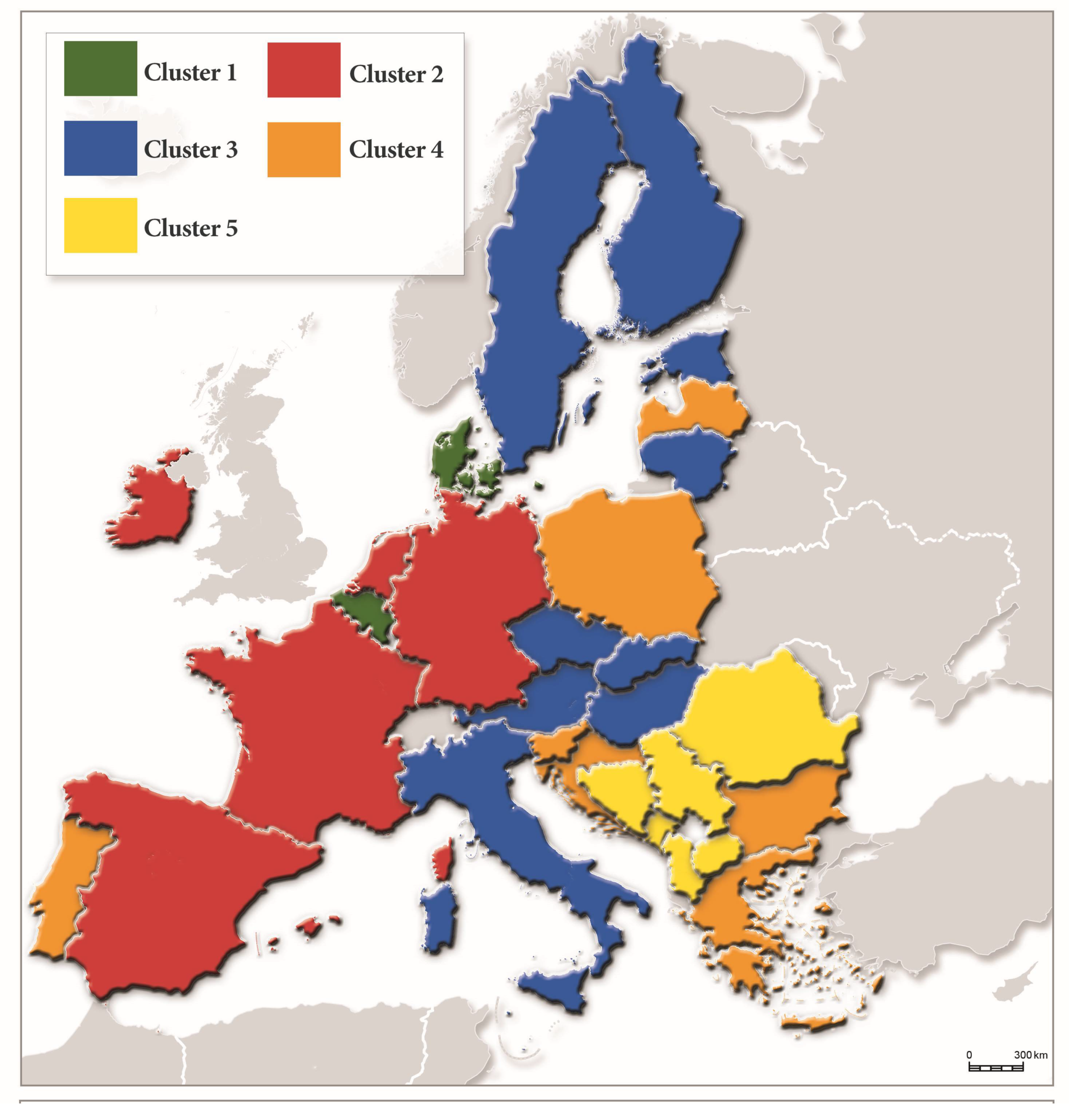
4.2. Cluster Analysis
5. Conclusions
Author Contributions
Funding
Institutional Review Board Statement
Data Availability Statement
Conflicts of Interest
Appendix A

| Authors/Year | Method | Country/Region | Output Variables | Input Variables |
|---|---|---|---|---|
| Latruffe at al. (2011) [46] | DEA | Hungary and France | Total output Milk produced COP output Other output | Utilized land, labor, capital, and intermediate consumption |
| Bojnec et al. (2014) [12] | DEA | Ten EU countries | Gross value added in $ | Labor, number of agricultural tractors, agricultural area, total fertilizers, and number of animal livestock units |
| Vlontzos and Niavis (2014) [13] | DEA and SFA | EU countries | total agricultural output | Agricultural land, labor and fixed capital consumption |
| Baráth and Fertő (2015) [47] | SFA | Hungary | total output | Labor, utilized agricultural area, total fixed assets in value, and total specific costs in value |
| Hart et al. (2015) [14] | SFA | 28 EU countries | agricultural GDP | Land, capital, fertilizer, labor, time, dummy variable country |
| Nowak et al. (2015) [10] | DEA | 27 EU countries | total output | Labor, capital, and land |
| Záhorský, T. and Pokrivčák, J. (2017) [17] | DEA | 10 CEEC countries | crop output animal output | Labor, utilized agricultural area, buildings, and fixed equipment, materials and total livestock units |
| Moutinho et al. (2018) [11] | DEA SFA | 27 EU countries | net added value | Inputs, labor force, utilized agricultural area, and energy consumed in the technical |
| Todorović et al. (2020) [20] | DEA | Serbia | total output | Total labor, utilized agricultural area, seed and plant costs, fertilizers, crop protection, farming overheads, depreciation, external costs, total assets, total liabilities |
| Đokić et al. (2020) [7] | DEA | Western Balkans and the New Member States | total output | Agricultural land, labor, and capital |
| Náglová and Rudinskaya (2021) [15] | SFA | 25 EU countries | total factor productivity | Land, labor, capital, and material |
Appendix B
| Parameter | Variable | Fixed Effects Model | Random Effects Model | ||
|---|---|---|---|---|---|
| Coefficient | Std. Error | Coefficient | Std. Error | ||
| Constant | −15.3896 a | 3.8088 | −23.3721 a | 2.8338 | |
| lnLabour | 0.0727 b | 0.0362 | 0.1260 a | 0.0301 | |
| lnLand | 0.1262 a | 0.0483 | 0.1600 a | 0.0404 | |
| lnGFC | 0.0864 a | 0.0199 | 0.0979 a | 0.0193 | |
| lnFertilizer | 0.0430 c | 0.0232 | 0.0579 b | 0.0227 | |
| lnLivestock | 0.4766 a | 0.0806 | 0.6688 a | 0.0450 | |
| time | 0.0106 a | 0.0015 | 0.0128 a | 0.0013 | |
| 0.5328 | 0.2681 | ||||
| 0.0659 | 0.0659 | ||||
| 8.0850 | 4.0683 | ||||
| 0.9849 | 0.9430 | ||||
| Number of observations | 372 | 372 | |||
| Number of countries | 31 | 31 | |||
| a statistical significance at level α = 0.01 b statistical significance at level α = 0.05 c statistical significance at level α = 0.1 | |||||
| Parameter | Variable | Fixed Effects Model | |
|---|---|---|---|
| Coefficient | Robust Std. Error | ||
| Constant | −15.3896 b | 60.643 | |
| lnLabour | 0.0727 | 00.568 | |
| lnLand | 0.1262 c | 00.635 | |
| lnGFC | 0.0864 a | 00.175 | |
| lnFertilizer | 0.0430 | 00.382 | |
| lnLivestock | 0.4766 a | 01.463 | |
| time | 0.0106 a | 00.023 | |
| 0.5328 | |||
| 0.0659 | |||
| 8.0850 | |||
| 0.9849 | |||
| Number of observations | 372 | ||
| Number of countries | 31 | ||
| a statistical significance at level α = 0.01 b statistical significance at level α = 0.05 c statistical significance at level α = 0.1 | |||
| Country | OTE | Country | OTE | Country | OTE |
|---|---|---|---|---|---|
| Albania | 0.3133 | France | 0.7318 | N. Macedonia | 0.3795 |
| Austria | 0.4417 | Germany | 0.7572 | Poland | 0.6622 |
| Belgium | 0.6346 | Greece | 0.6760 | Portugal | 0.4626 |
| Bosnia and Herzegovina | 0.2514 | Hungary | 0.6817 | Romania | 0.4987 |
| Bulgaria | 0.5496 | Ireland | 0.3101 | Serbia | 0.5443 |
| Croatia | 0.4043 | Italy | 0.7914 | Slovakia | 0.3619 |
| Czechia | 0.4649 | Latvia | 0.3125 | Slovenia | 0.2415 |
| Denmark | 0.5612 | Lithuania | 0.3943 | Spain | 0.7713 |
| Estonia | 0.2842 | Montenegro | 0.1414 | Sweden | 0.3864 |
| Finland | 0.3537 | Netherland | 0.6964 |
| OTE | Agricultural Land per Worker (ha/Worker) | Labor Productivity ($/Worker) | Land Productivity ($/ha) | |
|---|---|---|---|---|
| Cluster 1 | 0.60 | 32 | 148,860 | 5090 |
| Cluster 2 | 0.65 | 31 | 76,973 | 3556 |
| Cluster 3 | 0.46 | 25 | 37,127 | 1609 |
| Cluster 4 | 0.47 | 14 | 17,901 | 1481 |
| Cluster 5 | 0.35 | 10 | 8635 | 1116 |

References
- Zhao, Z.; Peng, P.; Zhang, F.; Wang, J.; Li, H. The Impact of the Urbanization Process on Agricultural Technical Efficiency in Northeast China. Sustainability 2022, 14, 12144. [Google Scholar] [CrossRef]
- Morais, G.A.S.; Silva, F.F.; Freitas, C.O.D.; Braga, M.J. Irrigation, Technical Efficiency, and Farm Size: The Case of Brazil. Sustainability 2021, 13, 1132. [Google Scholar] [CrossRef]
- Lazíková, J.; Lazíková, Z.; Takáč, I.; Rumanovská, Ľ.; Bandlerová, A. Technical Efficiency in the Agricultural Business—The Case of Slovakia. Sustainability 2019, 11, 5589. [Google Scholar] [CrossRef] [Green Version]
- Liu, J.; Dong, C.; Liu, S.; Rahman, S.; Sriboonchitta, S. Sources of Total-Factor Productivity and Efficiency Changes in China’s Agriculture. Agriculture 2020, 10, 279. [Google Scholar] [CrossRef]
- Zhu, Y.; Huo, C. The Impact of Agricultural Production Efficiency on Agricultural Carbon Emissions in China. Energies 2022, 15, 4464. [Google Scholar] [CrossRef]
- Matkovski, B.; Zekić, S.; Đokić, D.; Jurjević, Ž.; Đurić, I. Export Competitiveness of Agri-Food Sector during the EU Integration Process: Evidence from the Western Balkans. Foods 2022, 11, 10. [Google Scholar] [CrossRef] [PubMed]
- Đokić, D.; Zekić, S.; Jurjević, Z.; Matkovski, B. Drivers of technical efficiency in agriculture in the Western Balkans and New EU Memeber States. Custos Agronegocio Online 2020, 16, 2–15. [Google Scholar]
- Marcikić Horvat, A.; Matkovski, B.; Zekić, S.; Radovanov, B. Technical efficiency of agriculture in Western Balkan countries undergoing the process of EU integration. Agric. Econ. 2020, 66, 65–73. [Google Scholar] [CrossRef]
- Bakucs, Z.; Ferto, I.; Latruffe, L.; Desjeux, Y.; Soboh, R.; Dolman, M. Comparative Analysis of Technical Efficiency in European Agriculture. In Proceedings of the 2011 International Congress, Zurich, Switzerland, 30 August–2 September 2011. [Google Scholar]
- Nowak, A.; Kijek, T.; Domańska, K. Technical efficiency and its determinants in the European Union. Agric. Econ. 2015, 61, 275–283. [Google Scholar] [CrossRef] [Green Version]
- Moutinho, V.; Madaleno, M.; Macedo, P.; Robaina, M.; Marques, C. Efficiency in the European agricultural sector: Environment and resources. Environ. Sci. Pollut. Res. 2018, 25, 17927–17941. [Google Scholar] [CrossRef] [PubMed]
- Bojnec, Š.; Ferto, I.; Jambor, A.; Toth, J. Determinants of technical efficiency in agriculture in new EU member states from Central and Eastern Europe. Acta Oeconomica 2014, 64, 197–217. [Google Scholar] [CrossRef]
- Vlontzos, G.; Niavis, S. Assessing the Evolution of Technical Efficiency of Agriculture in EU Countries: Is There a Role for the Agenda 2000? Agric. Coop. Manag. Policy 2014, 339–351. [Google Scholar] [CrossRef]
- Hart, J.; Miljkovic, D.; Shaik, S. The impact of trade openness on technical efficiency in the agricultural sector of the European Union. Appl. Econ. 2015, 47, 1230–1247. [Google Scholar] [CrossRef] [Green Version]
- Náglová, Z.; Rudinskaya, T. Factors Influencing Technical Efficiency in the EU Dairy Farms. Agriculture 2021, 11, 1114. [Google Scholar] [CrossRef]
- Pawłowski, K.P.; Czubak, W.; Zmyślona, J. Regional Diversity of Technical Efficiency in Agriculture as a Results of an Overinvestment: A Case Study from Poland. Energies 2021, 14, 3357. [Google Scholar] [CrossRef]
- Záhorský, T.; Pokrivčák, J. Assessment of the Agricultural Performance in Central and Eastern European Countries. AGRIS Online Papers Econ. Inform. 2017, 9, 113–123. [Google Scholar] [CrossRef] [Green Version]
- Nowak, A.; Różańska-Boczula, M. The Competitiveness of Agriculture in EU Member States According to the Competitiveness Pyramid Model. Agriculture 2022, 12, 28. [Google Scholar] [CrossRef]
- Jarosz-Angowska, A.; Nowak, A.; Kołodziej, E.; Klikocka, H. Effect of European Integration on the Competitiveness of the Agricultural Sector in New Member States (EU-13) on the Internal EU Market. Sustainability 2022, 14, 13124. [Google Scholar] [CrossRef]
- Todorović, S.; Papić, R.; Ciaian, P.; Bogdanov, N. Technical efficiency of arable farms in Serbia: Do subsidies matter? New Medit 2020, 19, 81–97. [Google Scholar] [CrossRef]
- Jurjević, Ž.; Bogićević, I.; Đokić, D.; Matkovski, B. Information technology as a factor of sustainable development of Serbian agriculture. Strateg. Manag. 2019, 24, 41–46. [Google Scholar] [CrossRef]
- Matkovski, B.; Kalaš, B.; Zekić, S.; Jeremić, M. Agri-food Competitiveness in South East Europe. Outlook Agric. 2019, 48, 326–335. [Google Scholar] [CrossRef]
- Zekić, S.; Matkovski, B.; Kleut, Ž. Analiza agroekoloških indikatora u Srbiji i zemljama Evropske unije. Anali Ekon. Fak. Subotici 2018, 54, 45–57. [Google Scholar] [CrossRef]
- Tagarakis, A.C.; Dordas, C.; Lampridi, M.; Kateris, D.; Bochtis, D. A Smart Farming System for Circular Agriculture. Eng. Proc. 2021, 9, 10. [Google Scholar] [CrossRef]
- Erjavec, E.; Volk, T.; Rednak, M.; Ciaian, P.; Lazdinis, M. Agricultural policies and European Union accession processes in the Western Balkans: Aspirations versus reality. Eurasian Geogr. Econ. 2021, 62, 46–75. [Google Scholar] [CrossRef]
- Šeremešić, S.; Dolijanović, Ž.; Tomaš Simin, M.; Vojnov, B.; Glavaš Trbić, D. The Future We Want: Sustainable Development Goals Accomplishment with Organic Agriculture. Probl. Ekorozw. 2021, 16, 171–180. [Google Scholar] [CrossRef]
- Charnes, A.; Cooper, W.W.; Rhodes, E. Measuring the efficiency of decision making units. Eur. J. Oper. Res. 1978, 2, 429–444. [Google Scholar] [CrossRef]
- Kumbhakar, S.C.; Knox Lovell, C.A. Stochastic Frontier Analysis; Cambridge University Press: Cambridge, UK, 2003. [Google Scholar]
- Aigner, D.J.; Knox Lovell, C.; Schmidt, P. Formation and Estimation of Stochastic Frontier Production Function Models. J. Econom. 1977, 6, 21–37. [Google Scholar] [CrossRef]
- Meeusen, W.; van den Broeck, J. Efficiency Estimation from Cobb-Douglas Production Functions with Composed Error. Int. Econ. Rev. 1977, 18, 435–444. [Google Scholar] [CrossRef]
- Schmidt, P.; Sickles, R.C. Production Frontiers and Panel Data. J. Bus. Econ. Stat. 1984, 2, 367–374. [Google Scholar]
- Mundlak, Y. Empirical Production Function Free of Management Bias. J. Farm Econ. 1961, 43, 44–56. [Google Scholar] [CrossRef]
- Kumbhakar, S.C.; Lien, G.; Hardaker, J.B. Technical Efficiency in Competing Panel Data Models: A Study of Norwegian Grain Farming. J. Product. Anal. 2014, 41, 321–337. [Google Scholar] [CrossRef] [Green Version]
- Colombi, R.; Martini, G.; Vittadini, G. A Stochastic Frontier Model with Short-Run and Long-Run Inefficiency Random Effects; Working Paper Series; University of Bergamo: Bergamo, Italy, 2011. [Google Scholar]
- FAOSTAT. Available online: https://www.fao.org/faostat/en/ (accessed on 8 August 2022).
- FAO. Guidelines for the Preparation of Livestock Sector Reviews. Available online: https://www.fao.org/3/i2294e/i2294e.pdf (accessed on 8 August 2022).
- Hair, J.F.; Black, W.C.; Babin, B.J.; Anderson, R.E. Multivariate Data Analysis; Pearson: Upper Saddle River, NJ, USA, 2010. [Google Scholar]
- James, G.; Witten, D.; Hastie, T.; Tibshirani, R. An Introduction to Statistical Learning (with Applications in R); Springer: Berlin/Heidelberg, Germany, 2013. [Google Scholar] [CrossRef]
- Pallant, J. A Step by Step Guide to Data Analysis Using IBM SPSS; Taylor & Francis Group: London, UK, 2020. [Google Scholar]
- Battese, G.E.; Corra, G.S. Estimation of a production frontier model: With application to the pastoral zone of eastern Australia. Aust. J. Agric. Econ. 1977, 21, 169–179. [Google Scholar] [CrossRef] [Green Version]
- Levin, A.; Lin, C.-F.; Chu, C.-S.J. Unit root tests in panel data: Asymptotic and finite-sample properties. J. Econom. 2002, 108, 1–24. [Google Scholar] [CrossRef]
- Odeck, J. Measuring technical efficiency and productivity growth: A comparison of SFA and DEA on Norwegian grain production data. Appl. Econ. 2007, 39, 2617–2630. [Google Scholar] [CrossRef]
- Matkovski, B.; Zekić, S.; Jurjević, Ž.; Đokić, D. The agribusiness sector as a regional export opportunity: Evidence for the Vojvodina region. Int. J. Emerg. Mark. 2021. [Google Scholar] [CrossRef]
- Krstić, M.; Filipe, J.A.; Chavaglia, J. Higher Education as a Determinant of the Competitiveness and Sustainable Development of an Economy. Sustainability 2020, 12, 6607. [Google Scholar] [CrossRef]
- Reiff, M.; Surmanová, K.; Balcerzak, A.P.; Pietrzak, M.B. Multiple Criteria Analysis of European Union Agriculture. J. Int. Stud. 2016, 9, 62–74. [Google Scholar] [CrossRef]
- Latruffe, L.; Fogarasi, J.; Desjeux, Y. Efficiency, productivity and technology comparison for farms in Central and Western Europe: The case of field crop and dairy farming in Hungary and France. Econ. Syst. 2012, 36, 264–278. [Google Scholar] [CrossRef]
- Baráth, L.; Fertő, I. Heterogeneous technology, scale of land use and technical efficiency: The case of Hungarian crop farms. Land Use Policy 2015, 42, 141–150. [Google Scholar] [CrossRef]
- EUROSTAT. Available online: https://ec.europa.eu/eurostat (accessed on 8 August 2022).
- Agricultural Policy Plus—APP. Available online: http://app.seerural.org/ (accessed on 27 October 2022).


| Variable | VIF | TOL |
|---|---|---|
| lnLivestock | 8.94 | 0.1119 |
| lnFertilizer | 8.67 | 0.1153 |
| lnGFC | 6.09 | 0.1642 |
| lnLand | 5.50 | 0.1818 |
| lnLabour | 2.72 | 0.3678 |
| time | 1.03 | 0.9669 |
| Average | 5.49 | 0.3180 |
| Test | Null Hypothesis | Test Statistics | p-Value |
|---|---|---|---|
| Hausman test | Random individual effects model | 0.0000 |
| Variables | Null Hypothesis | Test Statistics | p-Value |
|---|---|---|---|
| lnVA | Presence of unit root | −96,160 | 0.0000 |
| lnLabour | Presence of unit root | −73,080 | 0.0000 |
| lnLand | Presence of unit root | −115,310 | 0.0000 |
| lnGFC | Presence of unit root | −93,710 | 0.0000 |
| lnFertilizer | Presence of unit root | −160,470 | 0.0000 |
| lnLivestock | Presence of unit root | −83,910 | 0.0000 |
| Test | Null Hypothesis | Test Statistics | p-Value |
|---|---|---|---|
| Modified Wald test | 0.0000 |
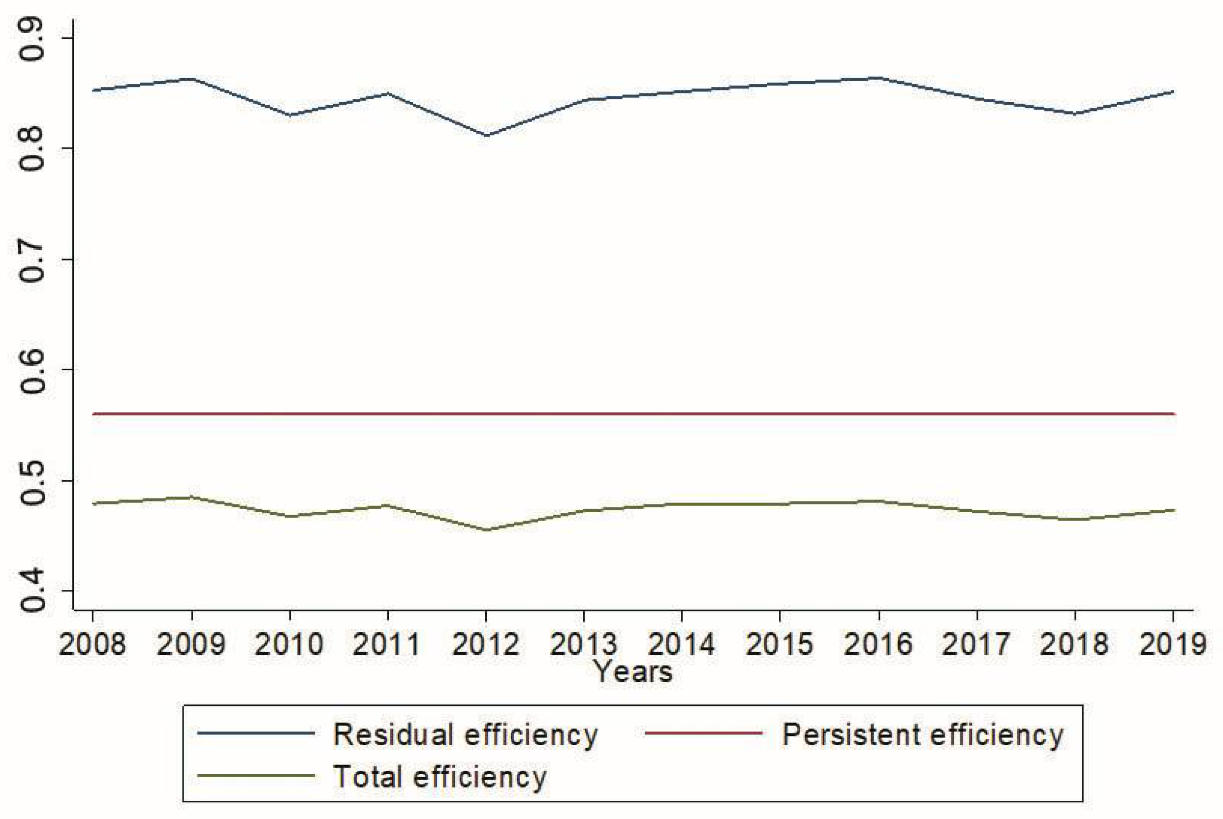
| TE | Number of Observations | Mean | Standard Deviation | Minimum |
|---|---|---|---|---|
| Residual | 372 | 0.8459 | 0.0524 | 0.6634 |
| Persistent | 372 | 0.5597 | 0.2220 | 0.1013 |
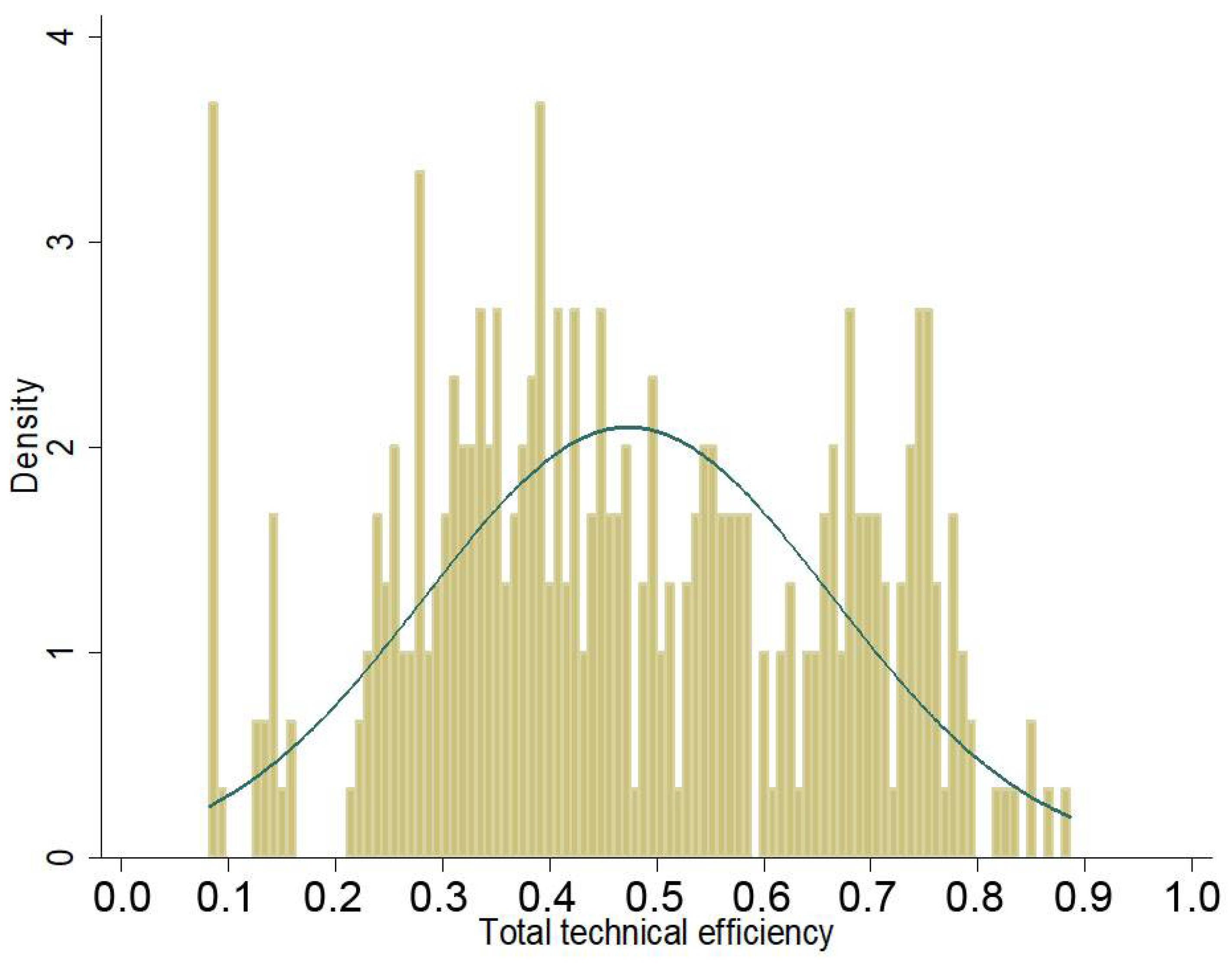
| Total | 372 | 0.4734 | 0.1900 | 0.0818 |
Publisher’s Note: MDPI stays neutral with regard to jurisdictional claims in published maps and institutional affiliations. |
© 2022 by the authors. Licensee MDPI, Basel, Switzerland. This article is an open access article distributed under the terms and conditions of the Creative Commons Attribution (CC BY) license (https://creativecommons.org/licenses/by/4.0/).
Share and Cite
Đokić, D.; Novaković, T.; Tekić, D.; Matkovski, B.; Zekić, S.; Milić, D. Technical Efficiency of Agriculture in the European Union and Western Balkans: SFA Method. Agriculture 2022, 12, 1992. https://0-doi-org.brum.beds.ac.uk/10.3390/agriculture12121992
Đokić D, Novaković T, Tekić D, Matkovski B, Zekić S, Milić D. Technical Efficiency of Agriculture in the European Union and Western Balkans: SFA Method. Agriculture. 2022; 12(12):1992. https://0-doi-org.brum.beds.ac.uk/10.3390/agriculture12121992
Chicago/Turabian StyleĐokić, Danilo, Tihomir Novaković, Dragana Tekić, Bojan Matkovski, Stanislav Zekić, and Dragan Milić. 2022. "Technical Efficiency of Agriculture in the European Union and Western Balkans: SFA Method" Agriculture 12, no. 12: 1992. https://0-doi-org.brum.beds.ac.uk/10.3390/agriculture12121992