1. Introduction
Chemical fertilizer is critical to boosting yield and efficiency in agricultural production. However, a low rate of fertilizer application will not favorably achieve the anticipated target. Moreover, overfertilization unavoidably reduces the utilization rate and affects the content of soil organic matter, leading to environmental issues such as soil hardening, acidification, and destruction of microbial systems. Therefore, various variable-rate fertilization studies have been carried out on quantitative fertilization in specific areas for proper field management [
1,
2,
3].
Currently, the fertilizer discharge mechanism of variable-rate fertilizer applicators mainly includes fluted-wheel type, centrifugal-disc type, and spiral-shaft type. Compared with the other two mechanisms, the spiral-shaft type demonstrates more adequate stability and uniformity of fertilization with varying rotational speeds [
4,
5,
6,
7]. It is necessary to consider the physical properties of fertilizer particles (density, size, shape, elasticity, looseness, etc.) and optimize the variation range of feeding length and the gap between the fertilizer discharge mechanism and the mechanism wall for determining the proper structure of the fertilizer applicator [
8]. The mechanism optimization can be conveniently executed using software simulation. Furthermore, as multi-purpose discrete element simulation software, EDEM can be used to analyze the impacts of different parameter combinations on the fertilization rate [
9,
10]. For instance, Chen et al. adopted EDEM to simulate the fertilization rate under diverse spiral angles and rotational speeds to enhance the accuracy and uniformity of fertilization [
11]. Tang et al. used EDEM to optimize parameters, including spiral-shaft dimension, spiral-blade radius, and pitch to achieve a satisfactory coefficient of variation of fertilization rate [
12]. However, there are no sufficient studies on the influences of the opening-length range of the fertilizer discharge mechanism and the gap between the spiral blades and the discharge cavity wall on fertilization performance.
Presently, the investigations on variable-rate fertilization focus on univariate fertilization and bivariate fertilization. The univariate fertilization is confronted with the deteriorated accuracy and uniformity of fertilization caused by the improper motor speed and the limited range of fertilization rate due to the single regulating parameter. Hence, researchers focus more on the modification of the fertilization rate by jointly controlling the opening length of the fertilizer outlet and the rotational speed of the fertilizer discharging shaft. Liu et al. developed a bivariate fertilizer applicator for rapid and precise fertilization using two direct current (DC) servo motors [
13]. Aaa et al. altered the opening length with pneumatic cylinders and the rotational speed by connecting the driven gear with the motor to expand the adjustment range of the fertilization rate [
14]. Although bivariate fertilization achieves a broader regulation scope than univariate fertilization, the nonlinear problem between variates and fertilization rate caused by the increased number of variates complicates the control system.
In addition, accuracy and uniformity are usually used as the assessment metrics of fertilization effectiveness [
15]. Currently, the advancement of fertilization performance of variable fertilizer applicators can be implemented by optimizing the decision-making and control systems. Yuan et al. established a fertilization control model based on a genetic algorithm (GA) optimized control combination using Gaussian process regression (GPR), with a mean relative error (MRE) of 0.089 [
16]. Nevertheless, the accuracy of fertilization is indirectly affected by the time lag as a result of the transition process of opening length and rotational speed. Thus, the decision-making algorithm should consider the adjustment time during the optimization of the control combination. Zhang et al. built a three-objective problem model with accuracy, uniformity, and adjustment time as the objectives and unraveled the difficulty of the optimal fertilization control decision through the multi-objective evolutionary algorithm based on decomposition (MOEA/D) based on the differential evolution (DE) algorithm to gain a superior MRE of 0.05977 [
17]. However, the method using MOEA/D for the solution of the multi-objective optimization model requires a considerably long running time to compute the fertilization decision in the actual scenarios. Moreover, various machine learning algorithms used to improve decision-making performance have different priorities in terms of computational efficiency, accuracy, and convergence speed, resulting in the requirement of global optimization for the whole variation range of variates during the determination of the control combination. The predicament causes many conventional optimization algorithms to drop into local optimum and requires considering the necessities of multiple objectives, failing to gain a reasonable accuracy of optimization results.
Swarm intelligence (SI) algorithms are gradually gaining prominence as more and more high-complexity decision-making problems require solutions within a reasonable time. Xue et al. proposed a new swarm optimization algorithm based on the behavior of group-living sparrows to achieve greater efficiency compared with other SI algorithms, although it has the shortcoming of easily falling into local extremum [
18]. Furthermore, Nguyen et al. recommended a modified sparrow search algorithm (SSA) utilizing the reverse learning strategy to enhance the accuracy and computational efficiency of multi-objective solutions [
19]. In addition, a chaotic operator and mutation section in a differential evolution (DE) algorithm are feasible and practical measures for SSA improvement. In this field, Wang et al. suggested an enhanced SSA in terms of global search capability and accuracy using Bernoulli’s chaotic maps [
20]. Moreover, Kathiroli et al. offered a DE-based SSA to promote computation efficiency and global search capability [
21].
Meanwhile, the control system regulates servo motors with closed-loop feedback consisting of a proportional–integral–derivative (PID) controller. The parameter-adaptive PID controller is widely investigated for reducing the inconvenience of empirical debugging and elevating the response speed and stability of the control system [
22]. For instance, Zhang et al. designed a variable-rate liquid fertilization control system using an improved PID algorithm and assessed the control performance with rise time and steady-state error [
23]. In addition, Bai et al. optimized the PID controller by adopting the integrated time absolute error (ITAE) criterion as a fitness function [
24]. However, the optimization or tuning process of these modified PID controllers struggles to balance operation speed and control stability, leading to unbearable computational complexity. The bat algorithm (BA) integrating the advantages of particle swarm, echo, and simulated annealing algorithms is undoubtedly one of the effective solutions to this difficulty [
25]. For example, Chaib et al. utilized BA to determine the parameters for optimizing the stability and response speed of a PID controller [
26]. Nevertheless, BA also tends to fall into local optimum, and a chaotic operator can be introduced to further facilitate the optimization of PID controller parameters.
To solve the aforementioned difficulty, a control combination decision-making method and control system is proposed to boost the operational performance of a bivariate fertilizer applicator in this study. Firstly, using EDEM software, the gap between the spiral blades and the discharge cavity and the range of opening lengths are optimized, and the fertilization process of the optimized variable-rate fertilizer applicator is precisely modeled. Secondly, utilizing the accuracy, uniformity, and adjustment time of fertilization as assessment criteria, the control combination optimization is determined by the SSA enhanced with a chaotic operator and mutation section of the DE algorithm. Finally, the PID controller optimized based on the improved BA is adopted to regulate the opening length of the fertilizer outlet and the rotational speed of the fertilizer discharging shaft.
The main contributions and innovations of this study are as follows:
The mechanical structure of a bivariate fertilizer applicator is optimized by EDEM software to avoid the loss and accumulation of fertilizer particles during the discharge process caused by inappropriate opening length and gap in the actual scenario.
The improved SSA using the chaotic operator and mutation section of the DE algorithm is used to promote global searching capability, accuracy, and convergence speed of control combination determination by diversifying the increasing population diversity and avoiding falling into the local optimum.
The parameter tuning of the PID controller with an improved BA using tent mapping is applied to reduce the rise time and the steady-state deviation for continuous variation in the control variable’s value.
2. Materials and Methods
2.1. Fertilizer Discharge Mechanism
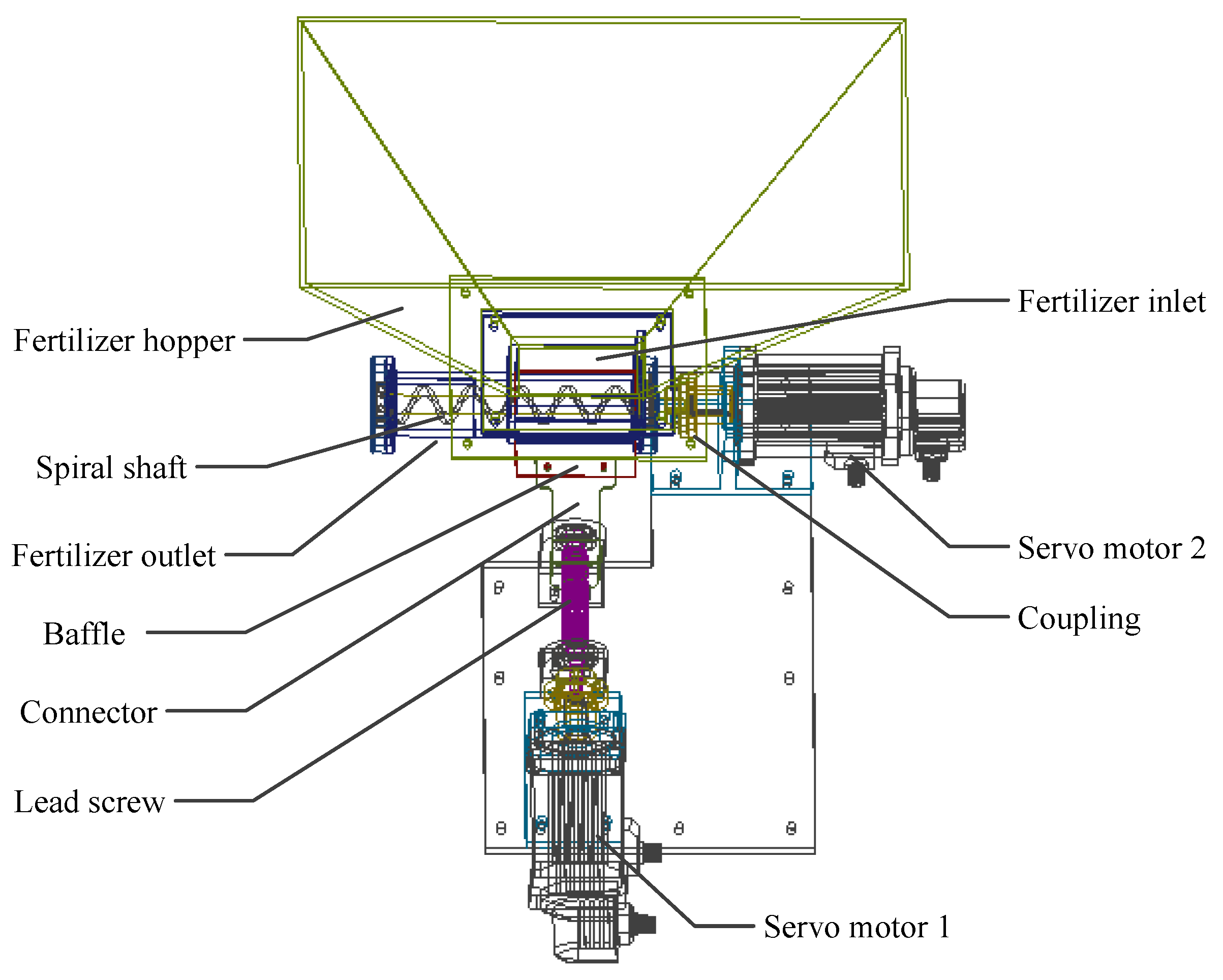
In this study, the designed test bench of the bivariate fertilizer applicator primarily consists of the fertilizer hopper, adjustment device of opening length, and rotational-speed control device. The main structure of the fertilizer applicator is assembled with 45-type steel. As shown in
Figure 1, the adjustment device of opening length (
L) is constituted by the baffle, connector, lead screw, and servo motor 1 (AKM41H-ANCNC-00, A&S Industry Technology Corporation, Boston, MA, USA). Since the screw pitch is set as 2 mm, the moving distance of the baffle is 1 mm in case the cylindrical rotor of servo motor 1 rotates half a turn. According to the forward and reverse rotation of servo motor 1, the lead screw is transformed into the linear reciprocating motion of the baffle to change the opening length through the connector. The rotational speed (
N) of the fertilizer discharging shaft is regulated directly by servo motor 2 of an identical model connected to the spiral shaft through a coupling, and the motor parameters are
R = 1.56 ohm,
Pn = 5,
Jm = 0.878 kg cm
2,
Ls = 5 mH. Therefore, the accurate fertilization rate is obtained by controlling two servo motors to output the expected opening length and rotational speed. The structure optimization of the essential mechanism parameters of the fertilizer applicator is required for acceptable fertilization performance before the test bench is assembled.
2.2. Parameter Optimization Based on EDEM
The parameter selection of the fertilizer applicator is undoubtedly critical to actual fertilization performance. Once the fertilizer applicator demonstrates significant instability at a small opening length, this leads to lowering accuracy. Meanwhile, the gap between the spiral blades and the discharge cavity can directly induce undesirable accumulation or overhead of fertilizer particles and is related to the regular work of spiral blades. Moreover, an insufficient gap will cause excessive friction while an oversized gap will decrease fertilizer discharge efficiency. As excellent multi-purpose discrete element simulation software, EDEM can be used to analyze the motion law of intricate discrete systems and to detect the impacts of particle size and particle flow on the equipment under study. In our study, EDEM is applied to achieve the minimum allowable opening length and the reasonable gap through simulation.
Prior to the parameter optimization, the essential physical performance parameters of fertilizers must be experimentally obtained or set by manual experience. The compound fertilizer (N-P2O5-K2O) used in this study has nitrogen content of 15%, phosphorus content of 15%, potassium content of 15%, and sulfur content of 10%, with a particle size of 3–5 mm and a slightly irritating odor. One hundred particles are randomly selected, and then the triaxial dimensions are measured by a digital vernier caliper (DL91150, Ningbo Deli Tools Corporation, China) with an accuracy of 0.01 mm. The volume ratio is defined as follows:
where
σ depicts the volume ratio of each fertilizer particle,
va expresses the volume of a fertilizer particle (mm
3), and
vb is the average volume of fertilizer particles (mm
3).
In addition, the density of fertilizer particles is estimated by the drainage method, the average angle of repose of fertilizer particle accumulation is calculated by the injection method, and the oven-drying method is adopted to obtain the moisture content of fertilizer granules. Meanwhile, the static friction coefficient between fertilizer particles and steel plate and the static friction coefficient between fertilizer particles are individually gauged by the plane method. Especially, the rolling friction coefficient is empirically determined as 0.01. Moreover, the collision restitution coefficient between the fertilizer particle and steel plate and the collision restitution coefficient between fertilizer particles are respectively achieved by the free-fall experiment. Furthermore, other parameters are designated according to manual experience, including density of 7890 kg m3, Poisson’s ratio of 0.3 and Young’s modulus of 209,000 GP for 45-type steel; Poisson’s ratio of 0.25 and Young’s modulus of 250 GP for fertilizer particles.
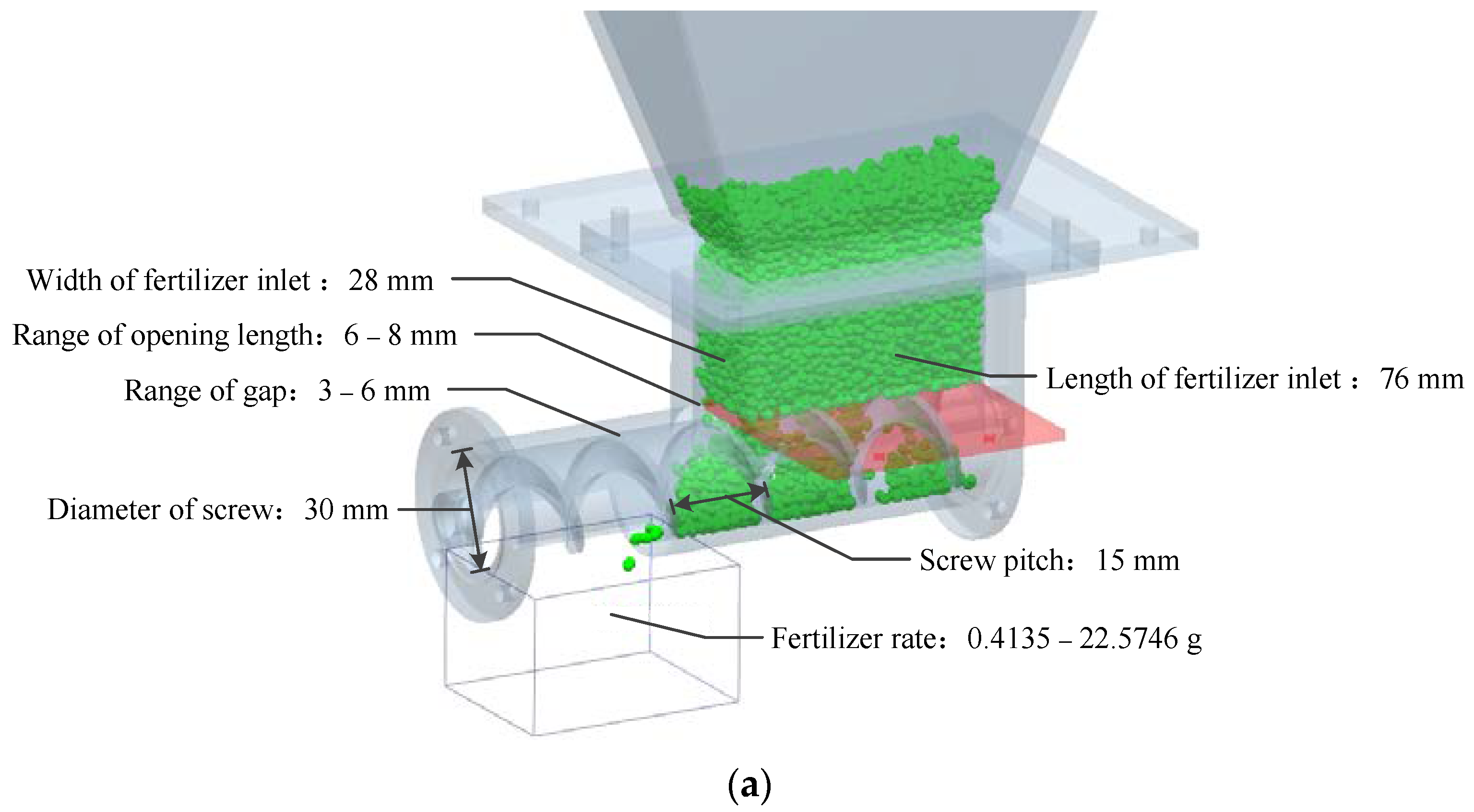
After the acquisition and configuration of the necessary parameters, the established 3D model of the bivariate fertilizer applicator is imported into the EDEM, and 500 g fertilizer is generated in the fertilizer hopper. In addition, the baffle and fertilizer discharging shaft are selected as moving parts. The search range of the minimum acceptable opening length is set from 5 mm to twice the diameter of fertilizer particles with an increment of 1 mm per time. Meanwhile, a virtual mass detector is used to weigh the discharged fertilizer, and the duration per simulation is assigned as 3 s (
Figure 2a).
Considering the diameter range of fertilizer particles and the deviation influenced by the coaxiality between the motor shaft and the fertilizer discharging shaft in actual operations, the gap between the spiral blades and the discharge cavity should be greater than 2 mm. Thus, the simulation range of the gap is designated as 3 to 6 mm, and the mixed fertilizer particles of random diameters are produced for the discharge performance test. In addition, the movement process of individual fertilizer particles of 3 to 5 mm is simulated under the selected gap scope for surveying the influence of the gap on the discharge status of the single particle (
Figure 2b). Eventually, the optimal range of opening length and the most suitable gap are acquired with the simulation comparisons.
2.3. Fertilization Data Acquisition
The test bench of the bivariate fertilizer applicator is built with the parameters optimized through EDEM. To establish the decision-making system, it is essential to measure the fertilization rates in case of various opening lengths and rotational speeds and assemble a fitting model to resolve the optimal combination of control variates. Therefore, indoor calibration experiments are conducted under stationary conditions to obtain fertilization data under different combinations of opening length and rotational speed. Due to the considerable growth variation in the fertilization rate at a small opening length, to accurately acquire the characteristics of the fertilization data, the size step of the opening length is set to 0.5 mm, 1 mm, and 2 mm for the ranges of 8–12 mm, 13–16 mm, and 18–28 mm, respectively. In addition, the variation range of the rotational speed is 10–150 r min
−1, and the step size is set to 10 r min
−1. The detailed ranges of opening length and rotational speed are listed in
Table 1.
It is easy to see that the total number of combinations of opening length and rotational speed is 285. Each combination is sampled 20 times, lasting for 30 s each time. The discharged fertilizer for each test is weighed, and the average fertilization rate per combination is recorded (
Supplementary Materials). Moreover, 10% of the experimental data are randomly selected as the test set, and the residual of the data is fitted with a polynomial curve fitting function. The data of the test set are compared with the predicted fertilization rate estimated by the fitting model, and the mean relative error (MRE) and coefficient of determination (R
2) are applied to assess the fitting effect. The most satisfactory fitting model of the fertilization rate is used as the fitness function of the decision-making algorithm.
2.4. Decision-Making Method for Fertilization-Rate Control
For the fitting model, there is a possibility that multiple combinations of opening length and rotational speed correspond to an identical target fertilization rate. At the same time, the control variates must be altered once the target fertilization rate is varied. Therefore, the maximum adjustment time of opening length and rotational speed is one of the principal factors affecting the response speed of the fertilizer applicator. Meanwhile, owing to the continuity of the fertilization process, the shorter the adjustment time, the lower the cumulative error of the fertilization rate. Furthermore, SSA is a novel swarm intelligence optimization method suggested by Xue and Shen. Aiming at the problem that SSA is prone to fall into the local optimum, the modified SSA based on a reverse learning strategy facilitates more efficiency than other machine learning algorithms and can avoid the severe limitation of tending to local extremum. In addition to using the reverse learning strategy, SSA can also be promoted by introducing a chaotic operator and mutation section in the DE algorithm.
Consequently, to overcome the above-mentioned difficulties, the improved SSA with a chaotic operator and mutation section of the DE algorithm is used in this study to optimize the control combination utilizing the adjustment time and fertilization accuracy as the evaluation criteria, and the fitness function is established with the difference between the fitted value of the fertilization-rate model and the expected fertilization rate. Specifically, the solution sets within 5% deviation of the target fertilization rate are probed by iteration. Then, the combination with the minimum discrepancy with the previous control combination is selected as the optimal regulation sequence. In particular, the fitness function of the improved SSA used to determine the control combination is defined as follows:
where
P denotes the predicted value achieved from the fitting model of fertilization rate, and
Q expresses the target fertilization rate.
The position coordinates of sparrows in the algorithm are formed by opening length and rotational speed. The position update formula for the predator during the population predation is described as follows [
27]:
where
xit is the two-dimensional coordinate of the
i-th individual of the population for the
t-th iteration,
T is the maximum number of iterations,
α is a random number in the interval of 0 to 1,
B is a normally distributed random number, and
V is a matrix of 1 ×
d with each element being 1. In addition,
R2 ∈ [0, 1] and
ST ∈ [0.5, 1] indicate the warning value and the safety threshold, respectively.
The position update formula for the intrant is depicted as follows [
28]:
where
C is a matrix of 1 ×
d with elements randomly being 1 or −1,
xwit is the worst position of the population of the
t-th iteration,
n is the population number, and
xbit+1 is the optimal position of the population of the
t + 1-th iteration.
The position update formula for the scouter is defined as follows [
29]:
where
β is a normally distributed random number with a mean value of 0 and a variance of 1,
K is a random number between −1 and 1, and
e is a minimal constant to prevent the denominator from being 0. Moreover,
fi means the fitness value of the
i-th sparrow,
fg and
fg signify the best and worst fitness values of the current sparrow population, respectively.
The introduced chaotic operator and mutation section of the DE algorithm are expressed as follows [
30,
31]:
where
z is a random number within [0, 1],
pop is the population size,
Tent(
x) is the value after chaotic mapping,
rand(
x) is a normally distributed random number with an expectation of 0 and a standard deviation of 1,
xj is the upper bound of the range of individual coordinates,
sj is the lower bound of the range of individual coordinates,
xat,
xbt, and
xct are the different individuals of the
t-th iteration, τ ∈ [0.5, 1] is the scaling factor, and
xnew is the position of new individuals after mutation operation.
During the search process, the improved SSA randomly generates various solutions from the local optimal solutions of each iteration by tent chaotic mapping and mutation section and computes the corresponding fitness values, and the individual with the best fitness is selected as the ultimate control combination. The parameters of improved SSA are shown in
Table 2.
The pseudo-code of the decision-making method of fertilization-rate control based on the improved SSA is illustrated in Algorithm 1.
| Algorithm 1 Decision-making method of fertilization-rate control using improved SSA |
| Input: Target fertilization rate S, population size pop, number of predators PNum, number of intrants JNum, number of scouters SNum, function dimension dim, iteration number T, previous control combination y. |
| Output: Optimal control combination (L, N). |
1. for each zi+1, i ∈ [0, 99] do
2. Compute points zi+1 using Equations (6) and (7)
3. end
4.
5. for each x(i,j), i ∈ [1, 100], j ∈ [1, 2] do
6. Compute fi using Equation (2)
7. return min fi, max fi, and xworse
8. end
9. xnew ← xbest
10. T = 1
11. while T = 100 do
12. for each , do
13.
14. end
15. st = rand(1)/2 + 0.5
16.
17. for each do
18. if then
19. Compute position of predators xi+1 using Equation (3)
20. else
21. Compute position of predators xi+1 using Equation (3)
22. end
23. end
24. for each do
25. if then
26. Compute position of intrants xi+1 using Equation (4)
27. else
28. Compute position of intrants xi+1 using Equation (4)
29. end
30. end
31. for each do
32. if then
33. Compute position of intrants xi+1 using Equation (5)
34. else
35. Compute position of intrants xi+1 using Equation (5)
36. end
37. end
38. for each x(i,j), i ∈ [1, 100], j ∈ [1,2] do
39. Compute fi using Equation (2)
40. end
41.
42. for each fi do
43. if fi > favg then
44. Compute xnew using Equations (6) and (7)
45. Compute fnew using Equation (2)
46. end
47. if fnew < fi then
48. fi ← fnew
49. xi ← xnew
50. end
51. end
52. T ← T + 1
53. end
54. for each do
55.
56. end
57. return
58. end |
2.5. Design of Fertilization-Rate Control System
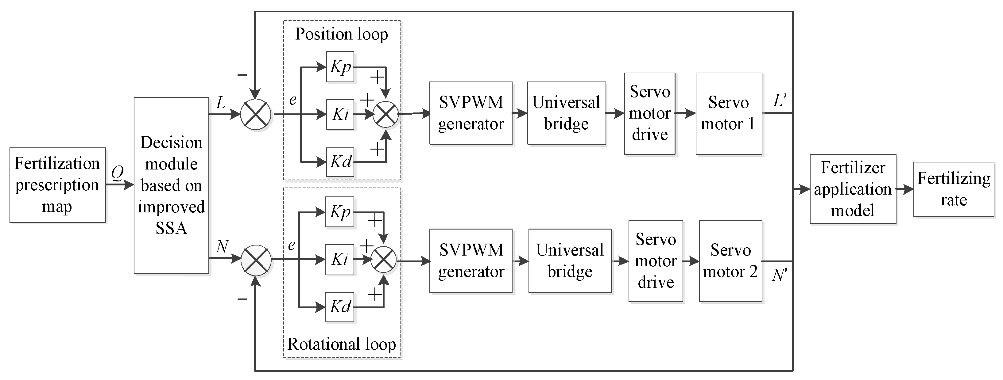
The control system of bivariate fertilizer applicators uses the optimal combination of opening length and rotational speed corresponding to the target fertilization rate as the input signal. At the same time, the feedback signals are sampled by a linear displacement sensor (optoNCDT1420, Mirco-Epsilon Measurement Corporation, Ortenburg, Germany) and a rotary encoder (E6C2-CWZ5B, Omron Tateisi Electronics Corporation, Kyoto, Japan), respectively. The difference between the input signal and the feedback signal is input into the PID controller optimized with the improved BA, and then the PID-regulated signal is employed as the q-axis current to import the space vector pulse width modulation (SVPWM) algorithm module after the inverse park transformation. Eventually, the voltage output adjusted by the regulation of the switching sequence and pulse width of the voltage source inverter using the SVPWM module is input to the servo motors for obtaining the desired opening length and rotational speed (
Figure 3).
In this study, the chosen servo motors are surface-mounted permanent magnet synchronous motors. Hence, the mathematical model in the synchronous rotating coordinate system
d–
q is selected to assemble the servo motor model, including the equations of the stator voltage, flux linkage, electromagnetic torque, and mechanical torque, as shown below [
32]:
where
ud and
uq are the
d–
q axis components of stator voltage, respectively;
id and
iq are the
d–
q axis components of stator current;
R indicates the resistance of the stator;
Te and
Tm are the electromagnetic torque and the mechanical torque, respectively;
Jm is the rotor inertia;
ψd and
ψq are the
d–
q axis components of stator flux, respectively;
ωe depicts the electromagnetic angular velocity;
Ld and
Lq are the
d–
q axis inductive components, respectively; and
ψf represents the permanent magnet flux.
In addition, the stator inductance satisfies the case of
Ld =
Lq =
Ls. Therefore, the stator voltage can be obtained from Formulas (9) and (10) as follows:
Since the control variate is directly related to the angle and rotational speed of the motor output, the conversion relationship between electromagnetic angular velocity
ωe, electromagnetic angle
θe, and motor speed
Nr is described as follows [
33]:
where
ωm is the mechanical angular velocity of motor rad s
−1,
Pn is the number of pole pairs, and
Nr is the motor speed r min
−1.
Moreover, the baffle position depends on the rotation angle of regulation motor 1, and the rotational speed of the fertilizer discharging shaft is determined by the speed of servo motor 2. Thus, the related transfer functions of the motor control are obtained by executing the Laplace transformation after merging Formulas (11) to (14), as shown below:
Afterwards, the following functions are obtained by substituting the specific motor parameters.
Following the construction of the transfer functions of servomotor control, the tent mapping bat algorithm (TBA) is used to optimize the PID controller by adding a tent chaotic operator in the iteration procedure for promoting the global search capability. Furthermore, the three parameters (proportion
Kp, integral
Ki, and differential
Kd) of the modified PID controller with the best control performance are solved with the minimum value of the ITAE criterion as the evaluation condition [
34,
35].
The position coordinates of individuals in TBA are composed of the PID controller parameters, and the frequency, position, and velocity of individual transformation are updated as follows [
36]:
where
fa is the frequency of the
i-th bat, randomly assigned during initialization.
vit denotes the velocity of the
i-th bat at the
t-th iteration,
xit indicates the position of the
i-th bat at the
t-th iteration,
xh signifies the current global optimal position, and
zi express the chaotic operator.
In the optimization procedure of the algorithm, individuals perform the random search in the vicinity of the present optimal solution while conducting a local search, and the position is updated according to the equation as follows [
37]:
where
xold is the current optimal solution,
xxin is the updated solution,
ε is a random number within [−1, 1],
At is the mean loudness of the bat population for the
t-th iteration.
With the increase in iteration number, the individual loudness
Ai gradually decreases, and the pulse emission frequency
r constantly grows. The update operations are implemented as follows [
38]:
where
a is the attenuation coefficient of loudness,
γ is the increasing coefficient of pulse emission frequency,
rib is the maximum of pulse emission frequency of the
i-th bat.
The parameters of TBA are shown in
Table 3. The detailed implementation process is shown in Algorithm 2.
| Algorithm 2 PID parameter optimization by improved BA |
| Input: Variation range of PID parameters, the maximum iterations tmax, population number n, initial loudness A, initial pulse emissivity r0, loudness attenuation coefficient α, increase coefficient of pulse emission frequency γ, population dimension d, initial velocity v, initial frequency fa, position of individual X, upper bound Ub and lower bound Lb, ITAE criteria evaluation value F, optimal individual position Xbest. |
| Output: Optimized PID parameters (kp, ki, kd). |
| 1. for i = 1:n do |
2. Xi ← Lb + (Ub − Lb).× rand(1,d)
3. Call sim function to return ITAE value based on the X value F ←
4. end
5. Xbest ← XI ← [Fmin, I] = min(F)
6. t = 0
7. while t < tmax do
8. i = t + 1
9. ri = r0 × (1 − e(−γ × t))
10. Ai = α × A
11. for j = 1:n do
12. Update frequency fa according to Equations (18) and (21)
13. Update the velocity v according to Formula (19)
14. Update the position of individual X according to Equation (20)
15. if rand < r do
16. X = Xbest + 0.1 × rand(1,d) × Ai
17. end
18. g = X < Lb
19. Xnew(g) = Lb(g)
20. h = X > Ub
21. Xnew(g) = Ub(h)
22. Call sim function to return ITAE value based on the Xnew value Fnew ←
23. if (Fnew < F) & (rand > A) do
24. X = Xnew
25. F = Fnew
26. end
27. if Fnew <= Fmin
28. Xbest = Xnew
29. Fmin = Fnew
30. end
31. t = t + 1
32. end
33. return (kp, ki, kd) ← (Xbest(1,1), Xbest(1,2), Xbest(1,3)) |
To test the performance of the PID controller designed for this study, the opening length and the rotational speed provided by the decision-making system are used as input signals and the simulation comparison with the PID control optimized based on BA, the conventional PID control, and fuzzy PID control, respectively, is implemented.
2.6. Assessment Criteria
Under the experimental condition of the same control system, the fertilization performance is verified through the test bench, and the target fertilization rate varies from 350 kg ha
−1 to 600 kg ha
−1 with an increment of 50 kg ha
−1. Meanwhile, the accuracy and convergence speed of the proposed decision-making algorithm, SSA, GA recommended by Yuan et al., and MOEA/D-DE suggested by Zhang et al. for control combination optimization are compared by the following evaluation criteria. The detailed parameters of GA and MOEA/D-DE are listed in
Table 4.
(1) Accuracy of fertilization
The accuracy is defined as the relative error (RE) between the measured value and the target value of fertilization rate and is defined explicitly as below:
where
ys is the fertilization rate obtained from the actual experiment, and
yg is the target fertilization rate.
(2) Uniformity of fertilization
The fertilization rate corresponding to each combination of opening length and rotational speed optimized by these decision-making approaches is measured 10 times for 30 s utilizing the test bench. The uniformity is evaluated through the coefficient of variation (CV) to indicate the dispersion degree of fertilizer particles during the fertilization process as follows:
where
ysd is the standard deviation of fertilization rate data, and
ym is the average fertilization rate. In particular,
ysd can be calculated by:
where
yi is the fertilization rate sampled at the
i-th measurement.
(3) Adjustment time
The maximum time needed to transition from the current fertilization rate to the following fertilization rate for modifying the opening length and rotational speed is used to describe the adjustment time. Obviously, the shorter the adjustment time is, the swifter the response of the fertilizer applicator will be.
To clarify the availability and effectiveness of the PID controller optimization using the improved BA, a series of comparisons with the fuzzy PID controller and the conventional PID controller is carried out by applying the opening length and rotational speed delivered from the decision-making method as the desired value. The specific descriptions of the assessment criteria are as follows.
(1) Accuracy
The accuracy of the controller is characterized as the steady-state deviation between the target value and the stable output value of the controller. The smaller the steady-state error value, the better the controller’s control performance.
(2) Response speed
The response speed of the controller is defined as the rise time required for the controller output to increase from 0.1 to 0.9 times the target value. The shorter the rise time, the more rapidly the controller responds.
3. Results and Analysis
The average volume of fertilizer particles is 19.835 mm
3 through the measurement and calculation of stochastically chosen samples, and the distribution proportions of the ratio of relative volume are exhibited in
Figure 4. It can be noticed that 72% of the selected fertilizer particles are within the range of 0.5–1.5, and these fertilizer particles are relatively regular and nearly ellipsoid in shape. On the other hand, 19% of the fertilizer particles are in the scope of 1.5–2.5 and much larger than the average volume. This phenomenon is caused by the irregular shape of fertilizer particles with bumps. In addition, 9% of the fertilizer particles are in the span of 0–0.5, and this portion usually has an anomalous cross-section.
The other physical characteristic parameters of fertilizer particles required in EDEM are gauged. Concretely, the density is 1.7163 g cm−3, the average angle of repose is 29.8°, and the moisture content is 5.278%. Meanwhile, the static friction coefficient between fertilizer particles and steel plate is 0.4592, and the static friction coefficient between fertilizer particles is 0.4998. In addition, the collision restitution coefficient between the fertilizer particle and steel plate is 0.427, and the collision restitution coefficient between fertilizer particles is 0.216.
The experimental results of fertilization performance using EDEM at small opening lengths are shown in
Table 5. It can be observed that the fertilization suspension occurs in different periods of the whole simulation process for the opening length of 5 mm, 6 mm, and 7 mm. In detail, more periods of fertilizer flow interruption emerge in the case of 5 mm, and the undesirable circumstance decreases with the growth of opening length. Contrarily, the fertilization process is smooth without discontinuous fertilizer flow at the opening length of 8 mm. The fertilization suspension in the simulation is induced by the extrusion and accumulation of irregularly shaped fertilizer particles at the position of the fertilizer outlet. This phenomenon can also boost the friction between fertilizer particles, resulting in a decline in the accuracy and uniformity of fertilization. Therefore, the minimum allowable opening length is selected as 8 mm.
The simulation results of fertilization rate for the variable gap between the spiral blades and the discharge cavity are displayed in
Table 6. In the simulation, the deviation of fertilization rate at the gap of 5 mm compared with the gap of 3 mm and 4 mm is 1.22 g and 1.51 g, respectively, the variation of that at the gap of 6 mm compared to the gap of 3 mm and 4 mm is 4.28 g to 4.57 g, and the fertilization-rate difference between the gap of 3 mm and the gap of 4 mm is 0.29 g. It can be seen that the fertilization rate drops with the boost of the gap value, and the fertilization rate is the minimum at the gap of 6 mm. This is because the diameter of fertilizer particles varying from 3 to 5 mm is less than the 6 mm gap value, meaning some fertilizer particles cannot be effectively propelled by the blade of the fertilizer discharging shaft. At the same time, the small gap (3 mm) can also reduce the transportation efficiency of the fertilizer discharging shaft. Thus, the gap value is designed to be 4 mm in the subsequent manufacturing process.
The fitting model of fertilization rate obtained by polynomial fitting is illustrated as follows:
where
P signifies the fertilization rate for the 30 s test period (g).
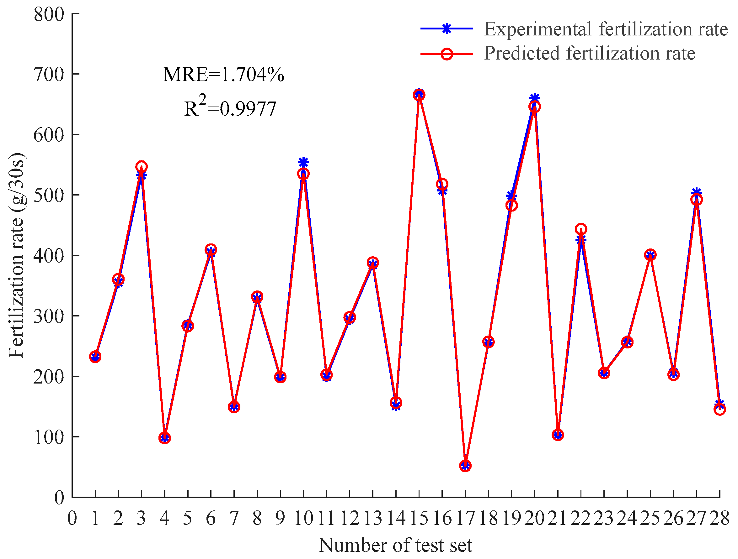
A total of 28 sets of data are randomly selected from the experimental fertilization data (
Table 7) to verify the accuracy of the fitting model. The opening lengths and rotational speeds of these test samples are imported into the model to achieve the predicted fertilization rates and then compared with the corresponding actual fertilization rates in the test data (
Figure 5). It can be found that the experimental fertilization rate under 400 g is remarkably proximate to the forecasted data of the model, while the actual fertilization-rate data above 400 g are slightly distinct from the predicted data of the model. This deviation is due to the manual adjustment of the polynomial second power and the coefficients before the variables for covering the fertilization-rate range suggested by agricultural specialists (150–250 kg ha
−1) through enhancing the accuracy of fertilizer application below 400 g [
39]. In addition, MRE is 1.704%, R
2 is 0.9977, indicating that the fitting model has tiny prediction variation and noteworthy accuracy.
The control combinations of the target fertilization rates optimized by these four optimization algorithms and the corresponding predicted fertilization rates acquired from the fitted model are shown in
Table 8. The maximum difference between the forecasted value corresponding to the control combination offered by the improved SSA, SSA, GA, and MOEA/D-DE and the target value is 6.2678 kg ha
−1, 9.1940 kg ha
−1, 2.0431 kg ha
−1, and 16.3877 kg ha
−1, respectively. Meanwhile, the minimum difference of that is 1.0756 kg ha
−1, 2.0088 kg ha
−1, 0.0233 kg ha
−1, and 8.9146 kg ha
−1, respectively, and the average difference of that is 3.9587 kg ha
−1, 5.6964 kg ha
−1, 0.6444 kg ha
−1, and 12.7799 kg ha
−1, respectively. The relative error of the difference relative to the target fertilization rate is 0.86%, 1.27%, 0.16%, and 2.69%. It can be seen that the optimization effect of GA is the best, while that of MOEA/D-DE is the worst. This is due to the diverse operation modes of these algorithms. GA pays more attention to accuracy. Conversely, the method used in this study, SSA, and MOEA/D-DE focus on the response time and weight parameter selection in control combination determination and is beneficial to the feasibility and practicality of application.
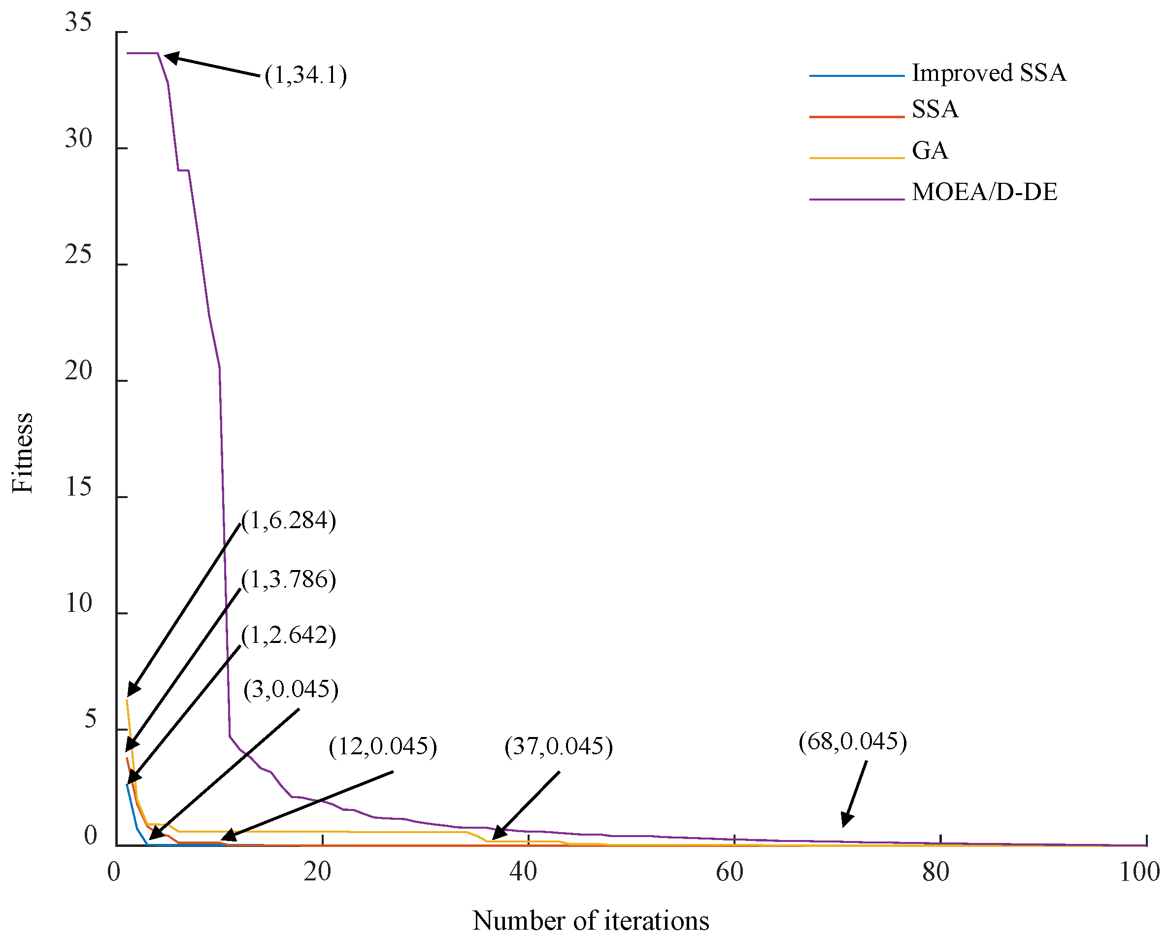
The convergence process of these four algorithms is depicted in
Figure 6. In the case that the iteration value equals 1, the fitness values of the proposed method, SSA, GA, and MOEA/D-DE are 2.642, 3.786, 6.284, and 34.1, respectively. When the fitness value reaches 0.045, the iteration values of the proposed method, SSA, GA, and MOEA/D-DE are 3, 12, 37, and 68, respectively. It can be noticed that the convergence speed of the proposed method is the fastest, and the MOEA/D-DE algorithm is the slowest. This is caused by the improvement of the SSA using a chaotic operator and mutation section of the DE algorithm that can reduce invalid iterations in the case of falling into the local optimal solution in the global optimization and accelerate the convergence speed.
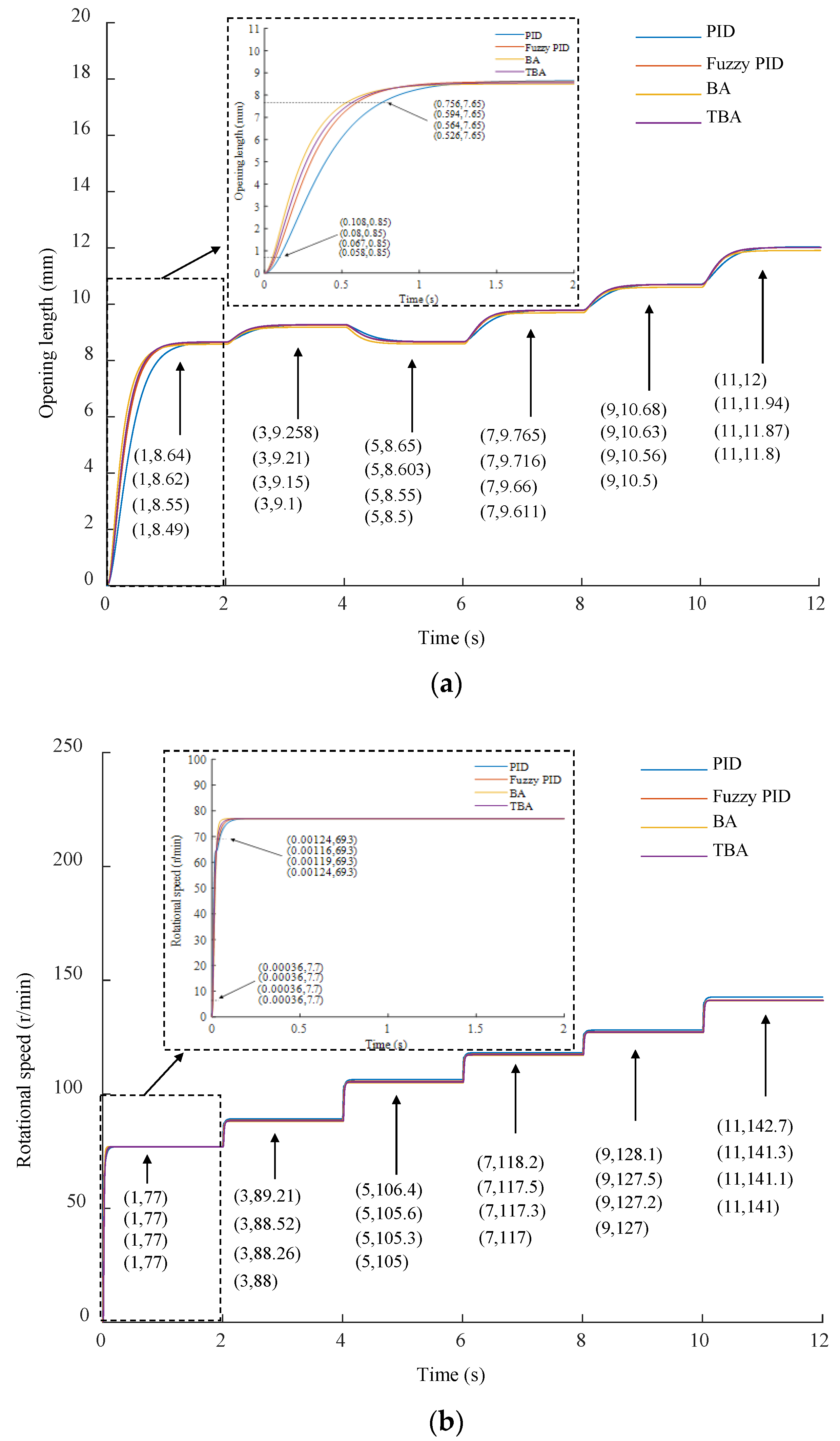
Taking the opening length and rotational speed offered by the decision-making algorithm when the target fertilization rate increases from 350 kg ha
−1 to 600 kg ha
−1 in increments of 50 kg ha
−1 as the desired values, the average accuracy of opening length of the PID controller optimized by TBA and the PID controller optimized by BA, the traditional PID controller, and the fuzzy PID controller is 0.004 mm, 0.057mm, 0.166 mm, and 0.120 mm, respectively. The average accuracy of the rotational speed of these four controllers is 0 r min
−1, 0.193 r min
−1, 1.102 r min
−1, and 0.403 r min
−1, respectively. In particular, for the target opening length of 8.5 mm, the response speed of output boosted from 0.85 mm to 7.65 mm is 0.468 s, 0.497 s, 0.514 s, and 0.648 s, respectively, and the steady-state deviations are 0.01 mm, 0.05 mm, 0.14 mm, and 0.12 mm, respectively. Moreover, for the target rotational speed of 77 r min
−1, the response speed of output increased from 7.7 r min
−1 to 69.3 r min
−1 is 0.0008 s, 0.00083 s, 0.00088 s, and 0.00088 s, respectively (
Figure 7). It can be discovered that the PID controller based on TBA optimization can accurately follow the shifts of the decision-making method. Therefore, compared with the PID controller based on BA, the traditional PID controller adjusting parameters through manual experience, and the fuzzy PID controller applying fuzzy rules for parameter tuning, the proposed PID controller in this study has a more acceptable control effect, which is slightly better than the controller optimized by BA.
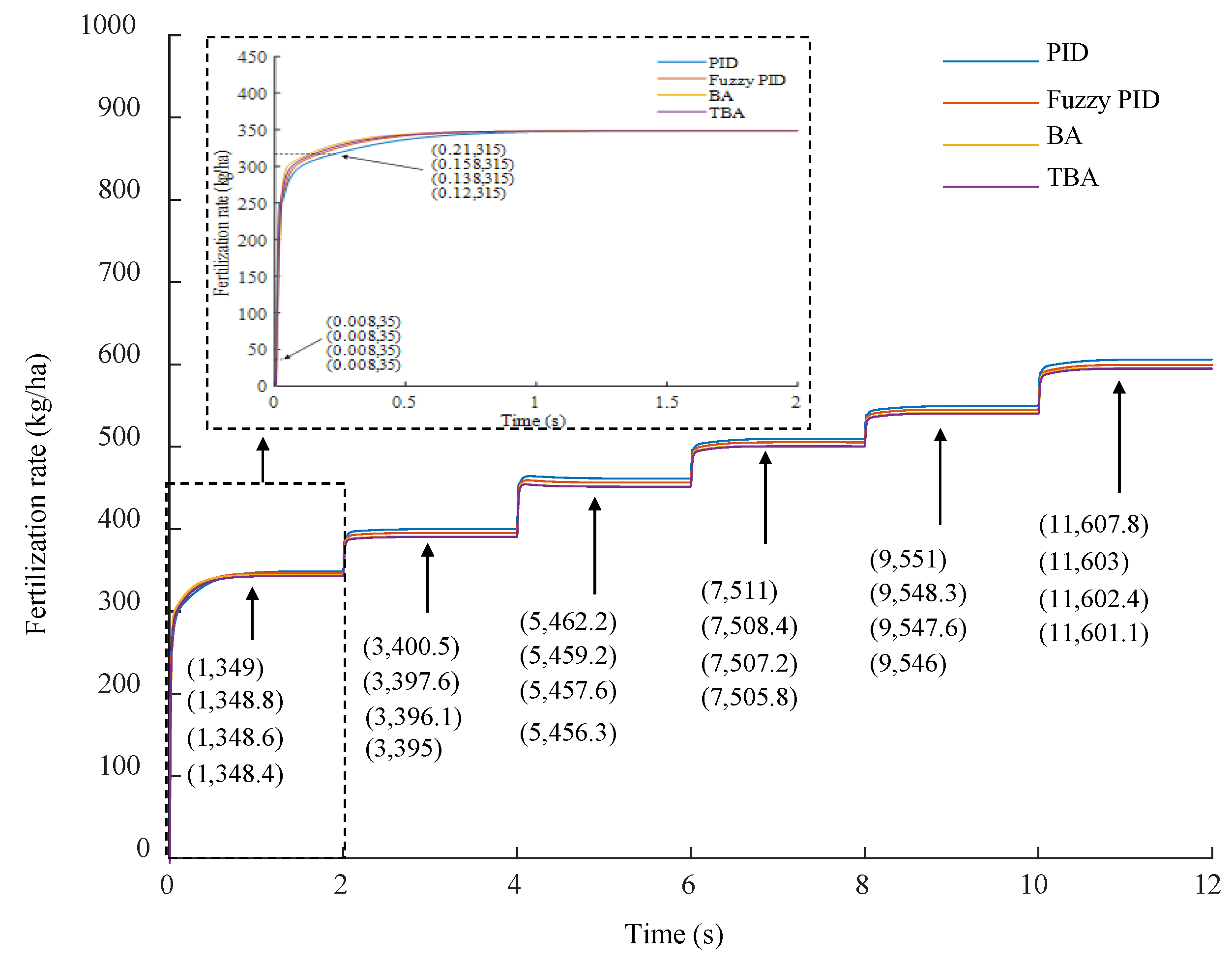
The corresponding simulation results of fertilization rate under the same conditions are demonstrated in
Figure 8. For the variable target fertilization rate, the average accuracy of the controller designed in this study, the PID controller improved by BA, the PID controller, and the fuzzy PID controller is 4.13 kg ha
−1, 4.15 kg ha
−1, 5.58 kg ha
−1, and 4.32 kg ha
−1, respectively. Obviously, the control performance of the PID controller optimized through TBA has a remarkably suitable outcome in terms of accuracy of fertilization and response speed. Especially, the rise time of fertilization rate, increased from 35 kg ha
−1 (0.1 × 350 kg ha
−1) to 315 kg ha
−1 (0.9 × 350 kg ha
−1), of the controller developed in this study, the PID controller improved by BA, the PID controller, and the fuzzy PID controller is 0.112 s, 0.13 s, 0.202 s, and 0.15 s, respectively. It can be found that the response speed of the proposed control system is optimal. In addition, the fertilization-rate adjustment is achieved by simultaneously regulating the opening length and rotational speed, and the rotational speed changes within the same time. Furthermore, in the short time that the fertilization rate grows from 35 kg ha
−1 to 300 kg ha
−1, the rotational speed can reach the target speed. However, the opening length is far from approximating the goal value, and the time used to boost from 300 kg ha
−1 to 350 kg ha
−1 is mainly generated by the opening-length adjustment. Therefore, the influence of the opening length on the equipment adjustment time is much more significant.
Under the same control system conditions, the indoor bench test is used to compare the performance of the control combination derived from these four decision-making methods on the bivariate fertilizer applicator. The indoor experimental data are indicated in
Table 9.
As shown in
Table 6, the average accuracy of the proposed method, SSA, GA, and MOEA/D-DE method is 1.8%, 1.9%, 2.5%, and 3.5%, respectively. The results suggest that the method proposed in this study performs most satisfactorily in terms of accuracy of fertilization. In addition, the average uniformity of the proposed method, SSA, GA, and MOEA/D-DE is 0.47%, 0.47%, 0.52%, and 0.48%, respectively, indicating that the proposed method had better uniformity than the other three methods, and the fluctuation of the fertilization process is slight. Moreover, since the indoor test is carried out with the same equipment, the unit adjustment time of the two variables is identical. The average adjustment time of the proposed method, SSA, GA, and MOEA/D-DE is 0.5 s, 0.99s, 1.48 s, and 1.34 s, respectively. Thus, the adjustment time of the method used in this study is more reasonable.


