
Recognition for Stems of Tomato Plants at Night Based on a Hybrid Joint Neural Network


College of Quality and Safety Engineering, China Jiliang University, No. 258, Xueyuan Street, Higher Education Zone of Xiasha, Hangzhou 310018, China
*
Author to whom correspondence should be addressed.
Agriculture 2022, 12(6), 743; https://0-doi-org.brum.beds.ac.uk/10.3390/agriculture12060743
Submission received: 14 April 2022
/
Revised: 16 May 2022
/
Accepted: 21 May 2022
/
Published: 24 May 2022
(This article belongs to the Special Issue Application of Robots and Automation Technology in Agriculture)
Abstract
:Recognition of plant stems is vital to automating multiple processes in fruit and vegetable production. The colour similarity between stems and leaves of tomato plants presents a considerable challenge for recognising stems in colour images. With duality relation in edge pairs as a basis, we designed a recognition algorithm for stems of tomato plants based on a hybrid joint neural network, which was composed of the duality edge method and deep learning models. Pixel-level metrics were designed to evaluate the performance of the neural network. Tests showed that the proposed algorithm has performs well at detecting thin and long objects even if the objects have similar colour to backgrounds. Compared with other methods based on colour images, the hybrid joint neural network can recognise the main and lateral stems and has less false negatives and positives. The proposed method has low hardware cost and can be used in the automation of fruit and vegetable production, such as in automatic targeted fertilisation and spraying, deleafing, branch pruning, clustered fruit harvesting and harvesting with trunk shake, obstacle avoidance, and navigation.
1. Introduction
The use of robots is the primary means for achieving automated production of fruits and vegetables and solving manufacturing problems such as labour shortages and high labour costs. Agricultural robots working at night have been investigated in recent years to prolong operation time and improve operation efficiency [1,2]. Vision systems are important in robots, where their main aim is to achieve the recognition and localisation of plant organs. In particular, the recognition of plant stems or branches of trees is of great importance and has high application value in multiple tasks, such as in automatic targeted fertilisation and spraying [3], deleafing [4,5], branch pruning [6,7,8], clustered fruit harvesting [9,10,11,12], harvesting with trunk shaker [13,14], obstacle avoidance [15,16], and navigation [17,18,19].
Three methods, namely, those based on colour image processing, multispectral image processing, and stereo vision, are prominent in the recognition of stems or branches. For the first method, colour images are acquired by using colour cameras, and these images are processed to recognise stems or branches [20,21,22,23]. For the second method, the recognition of stems can be realised on the basis of the grey difference between leaves and stems or branches in multispectral images, and this difference is caused by the moisture content between leaves and stems [24]. For the third method, stems or branches are usually recognised by using depth maps or point cloud processing. Depth maps or point clouds can be acquired by laser scanning [25], time-of-flight cameras [26], or stereo vision cameras [27].
Comparatively, the cost of the method based on colour images is low and can be applied and generalised easily. In current studies, this method is usually applied to recognise branches with colours different from those of leaves [28]. However, the recognition of stems or branches with colours similar to leaves is difficult. Several studies have been conducted on the recognition of stems with similar colours to their leaves based on colour images [3,29]. However, limitations are still found. This method is reliant on support ropes because stems are recognised by recognising the support ropes around which the stem is wrapped. Only the main stems can be recognised by using this method because they are wrapped around support ropes. The method based on multispectral image processing has an outstanding advantage in that it can recognise even stems or branches with similar colours to their leaves. However, the hardware cost is high. The method based on stereo vision can be used to recognise stems with similar colours to their leaves [26]. Although this method has good denoising performance for backgrounds far from plants, its performance for backgrounds close to plants encounters considerable problems. The depth image has no colour information, so the difficulty degree of image processing for branches with colours different from leaves is the same as that for branches with similar colours to leaves. The difference between depth images and colour images is only that pixel values in depth images are depth values and pixel values in colour images are colour values. Therefore, depth image processing methods are similar to the methods for colour images [30].
Deep learning methods have been widely applied in the recognition of plant organs. The three main tasks of deep learning methods are object detection [31], semantic segmentation [32] and instance segmentation [33]. Some studies have reported the recognition of plant organs with similar colours to backgrounds via deep learning. Most of them were applied in fruit detection [34], which is the task of object detection. Some of them were used to segment plants or plant organs [32] in images, which is the task of semantic segmentation. Tomato stem segmentation is a task of instance segmentation, which needs to segment different stem regions. Although deep learning has good recognition performance even for objects with similar colours to backgrounds, it has the disadvantages of more false negative errors due to the difficulties of learning the common features of stems in images with similar colours to backgrounds and variable illumination [35].
Many fruit and vegetable plants have stems or branches that are similar in colour to leaves. However, few studies have been published about recognition methods based on colour images for main and lateral stems or branches with similar colours to leaves. Recognition methods for stems or branches with similar colours to leaves are urgently needed.
The main purpose of this research was to design a recognition algorithm based on a hybrid joint neural network for stems of tomato plants with similar colours to leaves in colour images captured at night. The hybrid joint neural network is a class of neural network formed by the cascading and parallel connection of several networks. Other objectives were to design a recognition algorithm for stems on the basis of duality relation in edge pairs, train a recognition model based on mask region-based convolutional neural network (Mask R-CNN), and design a cascaded neural network composed of the duality edge method (DEM) and Mask R-CNN.
2. Materials and Methods
2.1. Testing Equipment and Image Acquisition
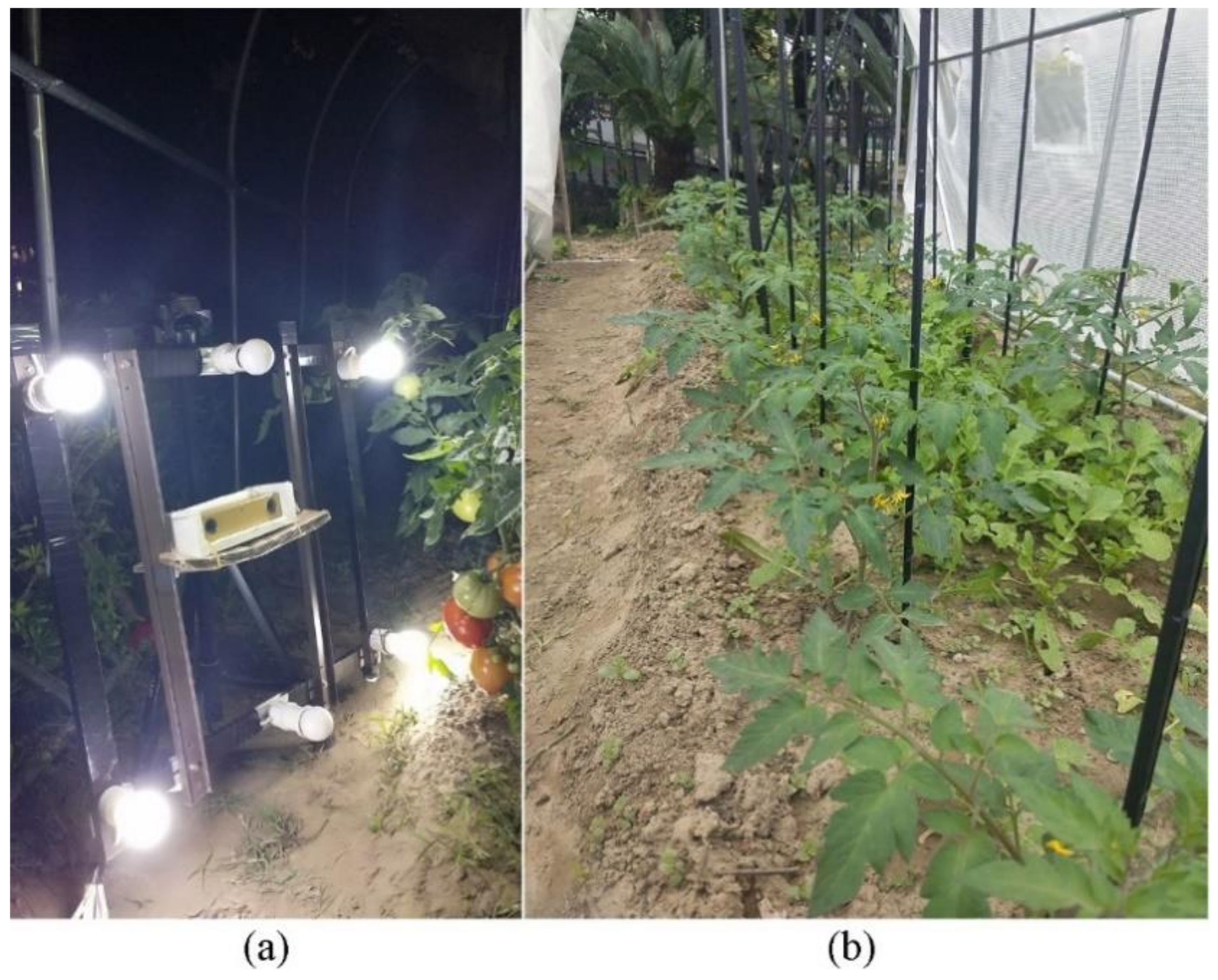
This study is a part of research on the recognition and localisation of stems of tomato plants at night. This study only focused on the recognition task of stems. This study used a binocular stereo camera to capture images of tomato plants for identifying the tomato stems. However, the 3D localisation of stems is a separate task and is not addressed in this study. The depth information was not used in this study. The camera model is Bumblebee2 made by Point Grey Research in Canada. Its image sensor is ICX204, and the focus length is 3.8 mm. The camera was mounted on a frame and connected to a computer by using a 1394 line and a MOGE 1394 capturer. The image resolution was 640 × 480 pixels. The binocular stereo camera can be replaced by a binocular stereo vision system constructed with two cheap colour cameras to reduce the hardware cost in future applications. The model of the computer is Lenovo R400. The illumination system is shown in Figure 1a. Four light sources (two 2 W light-emitting diodes [LEDs] and two 15 W incandescent lamps) and two layouts (up and down, and opposite) were used to construct different lighting systems and to evaluate the recognition performance of the algorithm for images captured under various lighting conditions. The programming environment was MATLAB R2017b.
Tomato plants were planted in a greenhouse, as shown in Figure 1b. The brightness varied in different parts of tomato plants under active lighting conditions at night, and lighting spot regions and dark regions appeared on the surface of stems. Tomato plant images were captured at night by using two illumination systems: two 2 W LEDs in up and down layout and two 15 W incandescent lamps in opposite layout. This process was performed to test the performance of the algorithm in adapting to various brightnesses. The shooting distances were 300, 450, and 600 mm.
2.2. Methods
The frame of the recognition algorithm designed for stems of tomato plants at night based on hybrid joint neural network is depicted in Figure 2.
The hybrid joint neural network was composed of a Mask R-CNN1 and cascaded neural network, which was made of a DEM and Mask R-CNN2. The two types of Mask R-CNN models have the same network structure and use different training sets for independent training. Mask R-CNN and the cascaded neural network can recognise the stem of tomato plants, as shown in Figure 2. Mask R-CNN has the disadvantages of more false negatives caused by bright or dim lighting conditions, but the coincidence degree between stem regions and the ground truths were high. On the contrary, the cascaded NN can reduce false negatives caused by bright or dim lighting conditions, but stem regions were thinner than the ground truths. The results of the two types of neural networks were combined to comprehensively utilised their advantages.
The cascaded neural network was composed of a method based on duality relation in edge pairs (hereinafter referred to as DEM) and mask R-CNN. To avoid confusion, we named the Mask R-CNN in the cascaded neural network as Mask R-CNN2, and the other one as Mask R-CNN1 in Figure 2. The DEM can recognise the stem of tomato plants. However, many false positives were found in the DEM results. Mask R-CNN2 was used to recognise stems from the DEM results to reduce false positives.
Mask R-CNN, the DEM, the cascaded neural network, and the hybrid joint neural network are separately introduced in the next subsections.
2.2.1. Mask R-CNN
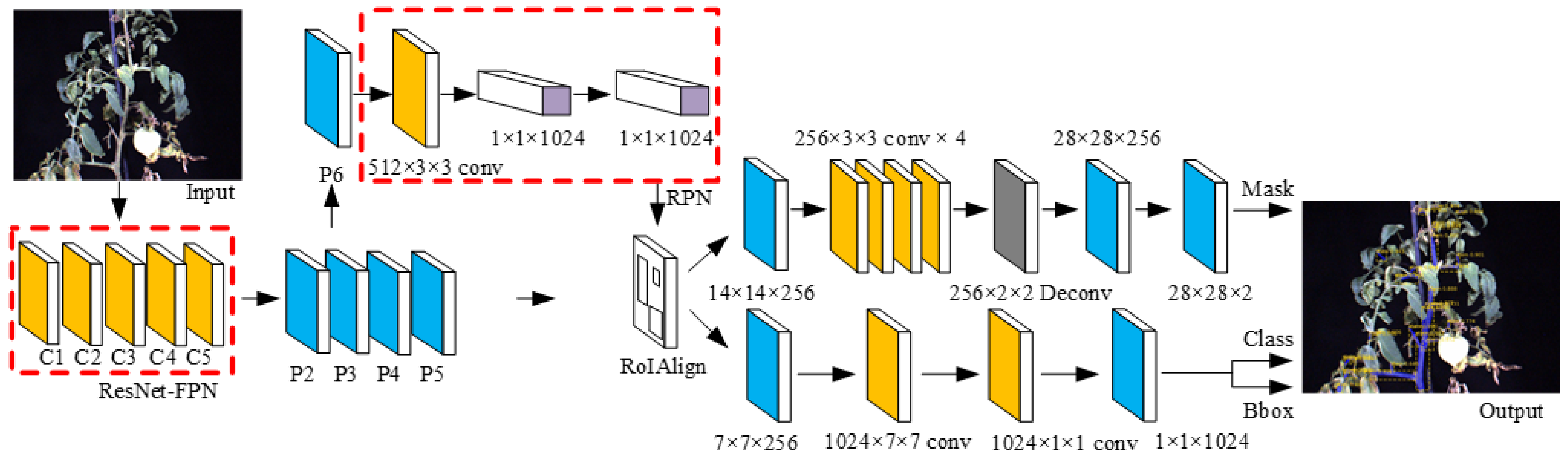
Mask R-CNN served as a deep learning framework of instance segmentation that can segment multiple targets simultaneously. It was composed of a backbone network, a regional proposal network (RPN) and three branches. The backbone network was used to extract the features of an input image to generate a feature map. The residual network Resnet101 and feature pyramid network (FPN) were selected as the backbone network. FPN was used to generate region of interest recommendation boxes for the region of interest. The feature maps involved in RPN were from the pyramid feature layer in FPN. The three branches included the class used for regression detection, the bounding box, and the mask of objects.
The deep learning environment was built by using deep learning frameworks TensorFlow 1.6.0 and Keras 2.1.6. (created by Google, Mountain View, CA, USA) Deep learning environment refers to the function package, which deep learning algorithms depend upon to run. Deep learning models, such as Mask R-CNN, are encapsulated in these function packages. TensorFlow and Keras are two famous deep learning environments in deep learning. Labelme software was used to label the tomato stems in images for producing a tomato stem data set. Table 1 shows the original and augmented datasets. Three types of geometric operations, namely, translation, flip, translation and flip, were used to obtain the augmented dataset. The total number of labelled stem objects in the three data sets exceeded 30,000. Transfer learning was introduced in this study to solve the problem of poor training effect and long convergence time of a small sample data set. A pretrained parameter model on the Microsoft Common Objects in Context (MS COCO) data set was used to initialise the Mask R-CNN network. MS COCO is a dataset built by Microsoft for image classification, object detection and semantic scene labelling tasks. Fine-tuning was performed on the whole network layer by combining the labelled tomato stem data sets to obtain the tomato stem recognition model at night. The optimal model parameters were as follows: initial learning rate of model training (0.001), momentum factor (0.9), weight attenuation coefficient (0.0001), step size of each iteration (506) and batch size (2). The anchor scale of RPN was 8, 16, 32, 64, and 128.
2.2.2. DEM
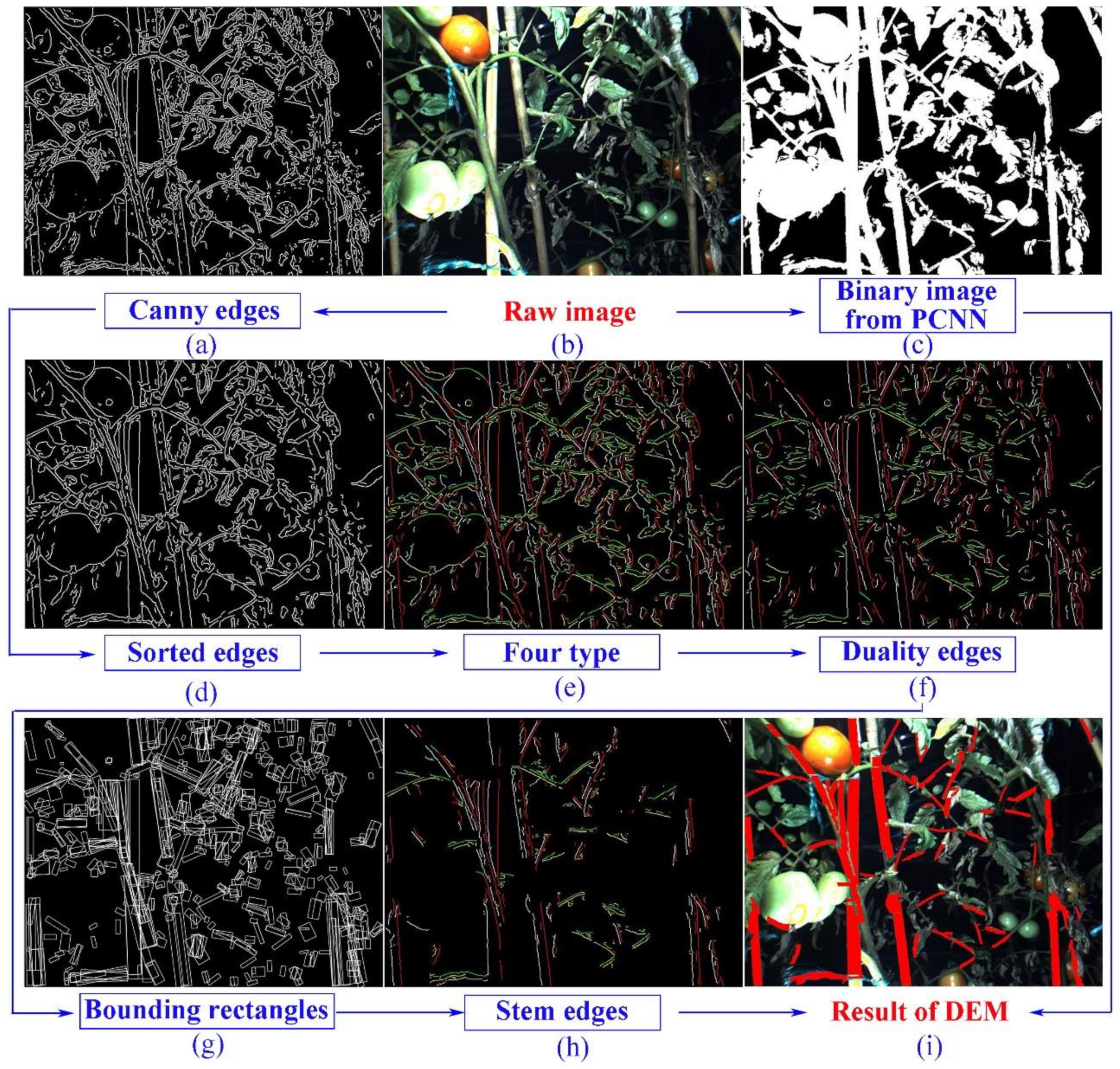
DEM involved eight steps, namely, image segmentation, edge extraction, edge sorting, edge type labelling, edge segmentation, stem duality edge extraction, stem edge recognition and stem region extraction. The first step, image segmentation, was used to segment the tomato plant. This step was performed on the basis of a pulse-coupled neural network (PCNN) which consists of coupling import area, internal activity area and pulser. The output of this segmentation step consists of segmented leaf regions. Steps 2 to 7 were performed to extract the stem regions based on the scheme of duality edge pairs. The extracted stem region was wider than that based on the PCNN. Therefore, the eighth step was used to combine the results of the first step and the seventh step, and the intersection of the two results was chosen as the final result. The advantage of the combining method is that the extracted stem region can be more accurate whilst removing the leaf area in the image segmentation result. The flowchart of the DEM is shown in Figure 3. The raw image and the DEM result are the same as in Figure 2. The eight steps are described in more detail.
- (1)
- Image segmentation
Image segmentation is the foundation of stem recognition. The purpose of the image segmentation algorithm is to segment the tomato plant as completely as possible.
This study adopted the segmentation method based on the simplified PCNN to realise image segmentation for tomato plant images. PCNN was designed on the basis of an underlying mechanism where similar stimuli evoke synchronous oscillation through the network, which can be interpreted as specific visual features [36,37]. In comparison with other machine learning models, the PCNN is an unsupervised learning method and has no training process. In comparison with other image segmentation algorithms based on threshold using only image greyscale value, PCNN uses spatial information and greyscale information to realise image segmentation.
The tomato plants are green in colour, which is strikingly different from the background. Therefore, the difference between green and red colours at every pixel was computed to segment tomato plants from backgrounds. The colour difference computation is the preprocessing step before the PCNN. Colour images were transformed into grey images after colour difference computation, and grey images were inputted to the PCNN. In this way, the PCNN can segment tomato plants accurately.
The principle of PCNN is described as follows: In an image with M × N pixels, PCNN takes a single pixel as a neuron. Pixel value is the external input stimulation of every neuron. Every neuron receives stimulation from the neighbourhoods. Two types of ignition, namely, natural ignition and captured ignition, are found for every neuron. The former renders the neuron active through external input stimuli, and the latter ignites neurons from their neighbours. Thus, ignited neurons activate their neighbours with similar visual inputs, forming a pulse wave that spreads within the network [37]. PCNN establishes a connection between similar pixels in the neighbourhood of the object and background regions and manages to segment them.
Given the complexity of the parameter setting of PCNN, OTSU was used to set the parameter automatically based on the threshold computed by OTSU [38]. OTSU is an adaptive threshold determination method based on the maximum between-cluster variance and is a common automatic threshold segmentation algorithm in computer vision and image processing.
Details about the improved PCNN based on OTSU can be found in Appendix A.
Figure 3c shows the segmentation result of Figure 3b using this algorithm and exhibits that the tomato plant can be segmented correctly.
- (2)
- Edge extraction
Canny algorithm was applied to extract tomato plant edges after comparison among several edge extraction algorithms (i.e., the Canny, Roberts, Sobel, Prewitt, and LOG operators). Details about the comparison among edge extraction algorithms are depicted in Appendix A.
Short edges were removed, and denoised edge images were acquired after edge extraction.
- (3)
- Edge sorting
Edge points on every edge should be sorted on the basis of their relative position relationship to recognise the stem edges of tomato plants. This process requires the longest edge (i.e., the main edge) and other edges (i.e., lateral edges) to be sorted separately.
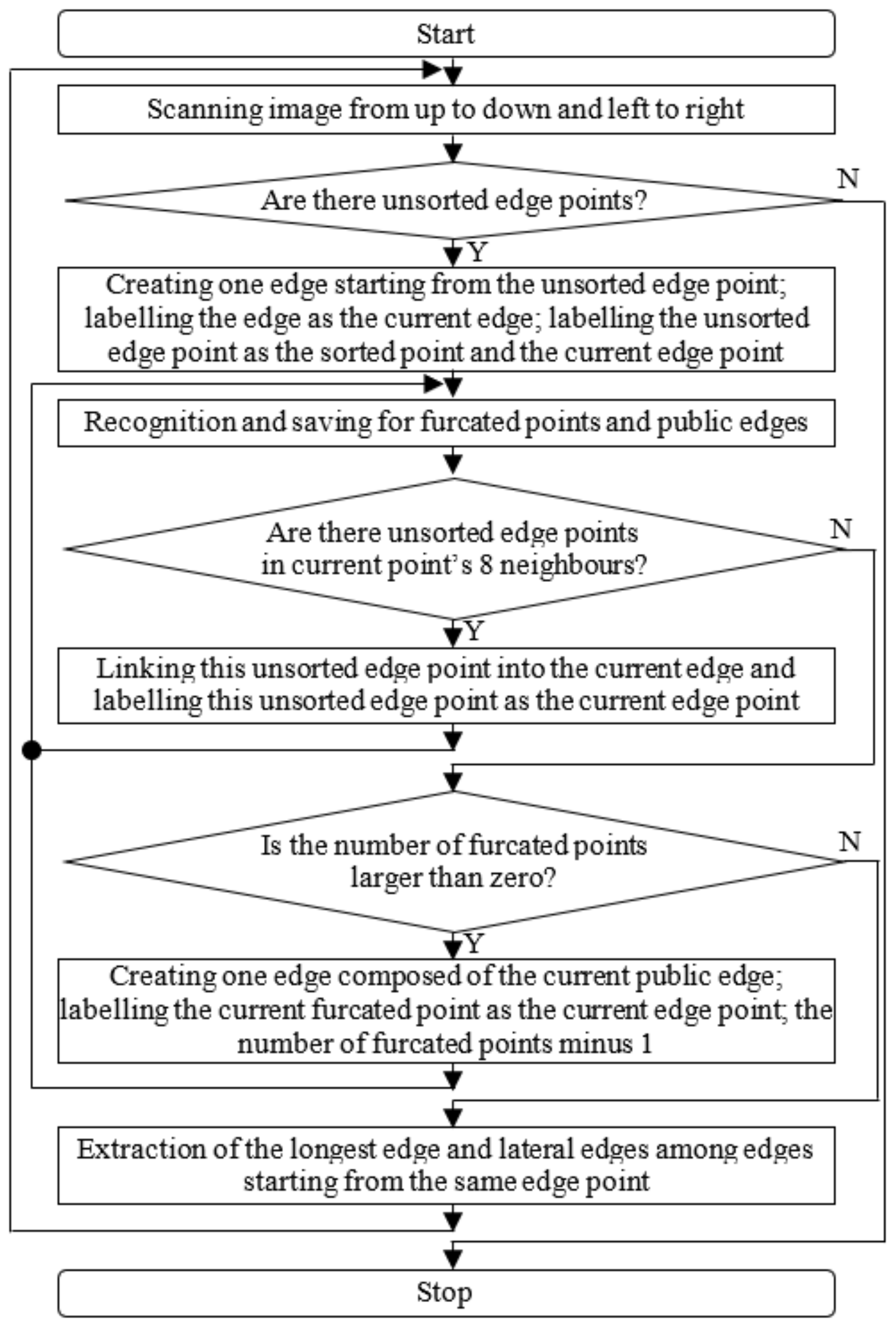
Edges intersect with each other, and the connection status of edges is complex because stems and leaves occlude each other. Thus, the method cannot meet the sorting required by these complex edges using traditional simple sorting algorithms that sort edge points in neighbour orders, such as 4 neighbourhood sorting or 8 neighbourhood sorting. In this study, we designed a new edge sorting algorithm applied to complex edges with fork points that can extract the longest sorted edge. Forked edges are extremely common in tomato plant edge images. The aim of seeking forked points is to extract the longest edge contained in each separated tomato plant region, thereby removing noise in the process. The flowchart of this edge sorting algorithm is illustrated in Figure 4. Details about the edge sorting algorithm can be found in Appendix A. Figure 3d illustrates the sorted results for edges in Figure 3a.
- (4)
- Edge type labelling
Points on sorted edges were labelled into four types, namely, up, down, left, and right, by using Equation (1) to realise edge segmentation after edge sorting.
where Elr (x, y) is the value of pixel (x, y) in the left and right type edge image Elr, the value of 1 indicates that the pixel belongs to the left type edge, and 2 denotes that the pixel belongs to the right type edge; Eud (x, y) is the value of pixel (x, y) in up and down type edge image Eud, the value of 1 indicates that the pixel belongs to the up type edge, and 2 denotes that the pixel belongs to the down type edge; Gx (x, y) is the x gradient value of the pixel with coordinates of (x, y) on the edge extracted by the Canny operator, and Gy (x, y) is the y gradient value of the pixel with coordinates of (x, y) on the edge extracted by the Canny operator.
However, many edge points that were up or down types in edge images of Eud and left or right types in edge images of Elr were acquired by using Equation (1). A new edge type-labelling algorithm based on Tl neighbour denoising was designed to realise unique labelling for every edge point. Details about edge type-labelling denoising algorithm are shown in Appendix A. Figure 3e shows the edge type labelling result of Figure 3d.
- (5)
- Edge segmentation
Every sorted edge was divided into different parts with varying edge types after edge type denoising. Thus, every edge can be segmented into several new edges at the point that its edge type differed from that of its front point.
- (6)
- Stem duality edge extraction
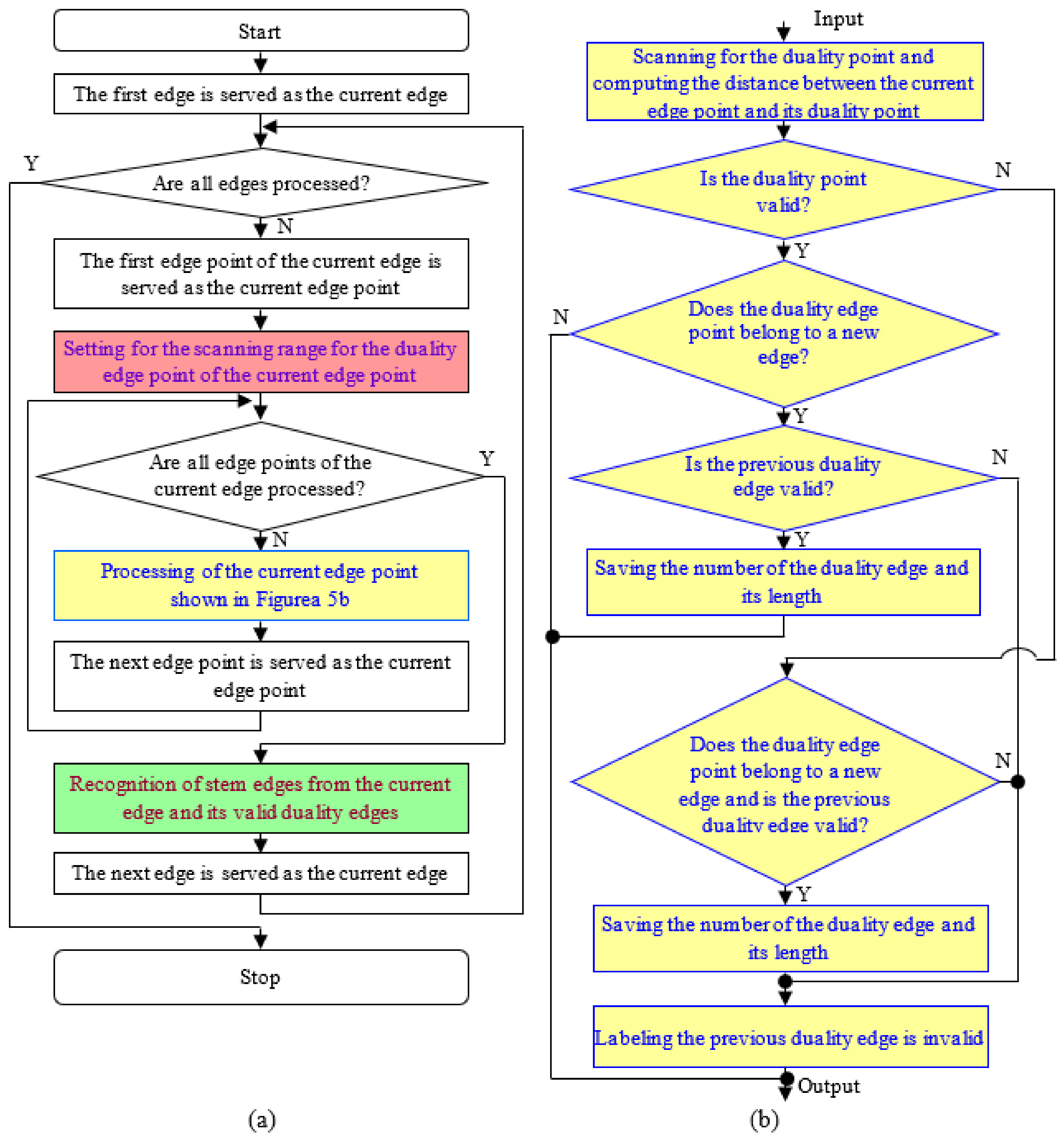
Duality exists at the edge of any object in an image. For example, if an object has a left edge, then it must have a corresponding right edge. If an object has an up edge, then it must have a corresponding down edge, vice versa. We defined this correspondence between the edges of objects as duality, defined a pair of edge points with duality as duality edge points, and defined a pair of edges with duality as duality edges. If the duality edge type is right, then it is scanned in the right orientational scanning range of the current edge point. Left is scanned in the left orientational scanning range, down is scanned in the down orientational scanning range, and up is scanned in the up orientational scanning range. For two edges in one stem edge pair (two edges of one stem region), one edge is the other’s duality edge, and they are complementary and united into one stem.
The distance between a stem edge pair is always smaller than that between a leaf edge pair (two edges of one leaf region). In edge images processed after edge segmentation, the distance between every edge point on one edge and its duality edge point on its duality edge were computed and denoted as t to recognise stem duality edge pairs. If all the values of t of all edge points on duality edge were smaller than Ty (set to 25 pixels based on the average diameter of stems in images), then the edge and its duality edges (more than one edge can be found) were extracted and served as stem duality edge pairs.
The flowchart of the extraction algorithm for the duality edge pairs of stems is shown in Figure 5. Several key points of the stem duality edge extraction algorithm are presented in Appendix A.
- (7)
- Stem edge recognition
Stem edge recognition
The minimum bounding rectangles of duality edges were extracted to extract shape features of every pair of duality edges. Figure 3g shows the bounding boxes of duality edges in Figure 3f.
Equation (2) shows the computation of the shape feature of the length–width ratio of the minimum bounding rectangles of duality edges.
where r is the length–width ratio of the minimum bounding rectangles of duality edges, l is the length of the minimum bounding rectangles of duality edges, and w is the width of the minimum bounding rectangles of duality edges.
r= l/w
If the value of r is larger than Tr, then the duality edges belong to stem edges. Otherwise, the duality edges belong to nonstem edges. On the basis of comparison tests, the value of Tr was set to 4.5.
Figure 3h shows the recognition result of Figure 3f. Stem edges were recognised successfully by using this shape feature.
- (8)
- Stem region recognition
The task of this step is to transform the recognised duality stem edges into stem regions. The stem region was recovered by the pair of duality edges of stem and the average distance between its duality edges, and the diameters at two ends of the same stem were different, especially the main stem. Thus, half of the recovered stem was wider than the ground truth. Therefore, the intersection of the stem region and its PCNN image segmentation result was regarded as its recognised stem region to obtain a more accurate stem region. Details about the stem region recognition algorithm are shown in Appendix A.
2.2.3. Cascaded Neural Network
The cascaded NN in the study was composed of the DEM and Mask R-CNN. Raw images were the DEM inputs, and the DEM output was the input of the Mask R-CNN module. This architecture allowed comprehensive utilization of the advantages of the two algorithms and made it possible to eliminate the false positives that resulted from the DEM stage.
Figure 2 shows that the precision rate is good for the method of Mask R-CNN. However, many false negatives were obtained. The recall rate was good for the DEM, but many false positives were observed. Specifically, the DEM can detect stems, which cannot be detected by the Mask R-CNN, and the Mask R-CNN can detect nonstems, which cannot be detected by the DEM.
The model of the Mask R-CNN used in the cascaded net was the same with that described in Section 2.2.1. Details about the model of the Mask R-CNN can be found in Appendix B. The difference was that the data sets used in the cascaded net were composed of images resulted from the DEM. Labelme software was used to label the stems in images to produce the data sets.
2.2.4. Hybrid Joint Neural Network
The hybrid joint neural network was combined through an ‘or’ operation between the cascaded NN and the Mask R-CNN. As illustrated in Figure 2, such a combination improves the recognition of the stem regions otherwise reconstructed thinner than the ground truth.
3. Results and Discussion
The performance of the hybrid joint neural network was tested. For performance comparison, the DEM, Mask R-CNN, cascaded neural network composed of the DEM and Mask R-CNN, YOLACT, and cascaded neural network composed of the DEM and YOLACT were tested. You Only Look at CoefficienT’ (YOLACT) is a real-time instance segmentation model. It was used for performance comparison test in this study.
3.1. Performance Evaluation Methods for the Recognition Algorithm
False negative and false positive errors were found amongst the recognition results. The former indicates that stem pixels are falsely recognised as other organ pixels. False positive denotes that other organ pixels are falsely recognised as stem pixels.
In this study, we used the precision rate, recall rate, and F1 value based on pixel-level (uncommon metrics based on object level) to evaluate the performance of the algorithm, which were computed as Equations (3)–(5) separately.
where P is the pixel-level precision rate, TP is the pixel-level true positive, FP is the pixel-level false positive, R is the pixel-level recall rate, FN is the pixel-level false negative, and F1 is the pixel-level F1 value. ‘TP + FP’ indicates the union of the TP and FP, and is the recognition result. ‘TP + FN’ denotes the union of the TP and FN, and is the ground truth.
P = TP/(TP + FP)
R = TP/(TP + FN)
F1 = 2PR/(P + R)
The difference between the pixel-level metrics and the object-level metrics was the unit of calculation. The former was used to compute the TP, FP, and FN in pixels. The latter was computed on the basis of objects. Object-level metrics suggest that the model has the same performance in identifying a large-area stem as it does in identifying a small-area stem. In this study, the model performed better at identifying a large-area stem than at identifying a small-area stem. Therefore, pixel-level metrics were used to evaluate the model performance more accurately.
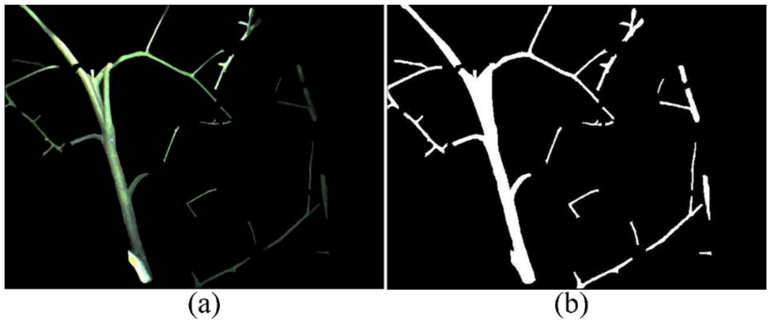
True positive is the intersection of ground truth and recognition results. The ground truth was acquired by sectional drawing using Photoshop software. Figure 6a shows the ground truth of stems in Figure 3a. Figure 6b show its binary image. Therefore, TP + FP is the area of recognition results, and TP + FN is the ground truth. TP is the area of the intersection of the ground truth and recognition results.
Pixel-level metrics are more accurate than common object level metrics because stems with different areas cannot be assigned the same weight to evaluate the performance of the algorithms in this study. Stems with large areas should be assigned heavy weights due to the great influence on algorithm performance evaluation. However, pixel-level metrics are strict. The performance evaluated by pixel-level metrics is worse than the actual performance. Pixel-level metrics decrease when the recognised stem region is thinner than its ground truth. However, in this situation, if the length of the recognised region is close to the length of its ground truth, then the recognised stem region can still represent its ground truth in a deleafing application.
3.2. Recognition Performance
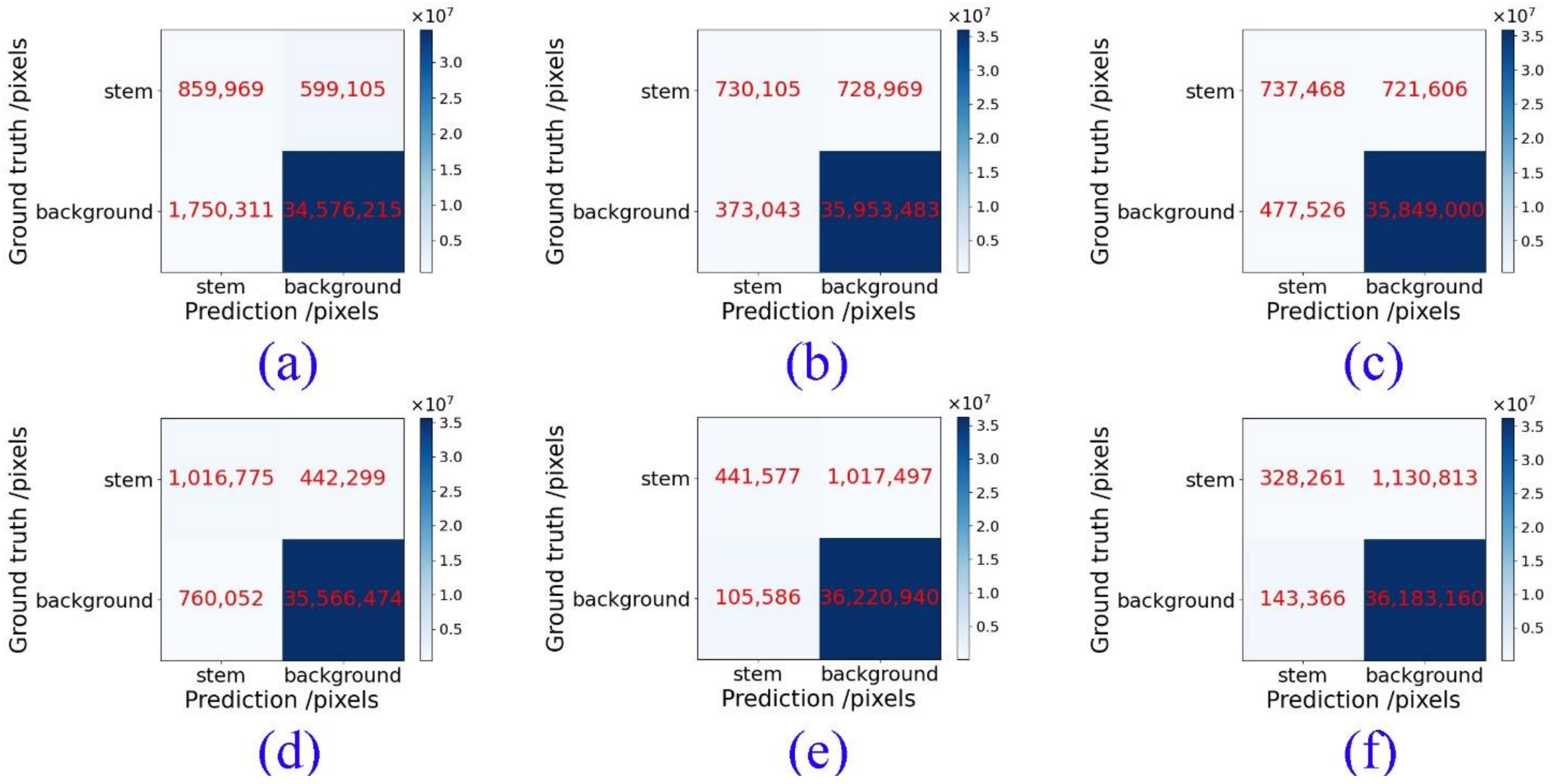
The recognition results of tomato plant images were computed by using six methods. The confusion matrices of test results are shown in Figure 7. The precision rate (P), recall rate (R) and F1 value (F1) were computed on the basis of the confusion matrices. The results are shown in Table 2.
Table 2 indicates that stems are correctly recognised in 57.2%, 69.7%, and 62.8% of the average precision rate, recall rate and F1 value.
The precision rate must be improved because of false positive errors. Two types of false positive errors were noted. One was caused by supporting poles, and the other was caused by leaves. For the first type, the shape features between stems and supporting poles were extremely similar, which can be solved by replacing the supporting poles with others, such as supporting lines. The algorithm demonstrated good potential to recognise thin and long objects with similar colour to their backgrounds. For the second type, edges in a leaf edge pair were straight, and the width of a leaf edge pair was small, so the leaf edge pair was falsely recognised as stem edge pair. Given the similar colours between leaves and stems for tomato plants, recognising stems from leaves is challenging.
The test results showed that the recall rate was low due to false negative errors. The false negative errors were due to several reasons. Firstly, false labelling of edge type in the DEM method resulted in false recognition. One reason was that one edge was falsely labelled into different types, so this edge was divided into several short edges. Another reason was that neighbouring edges with different edge types were labelled under the same type. Neighbouring edges were falsely merged into one, and this merged edge curve resulted in false negatives. Secondly, stems were completely or mostly occluded by leaves and fruits with similar colour, thereby resulting in information missing. If only few parts were visible, then the stems were falsely recognised as leaves. Thirdly, the lighting conditions resulted in false negatives. One reason was that the intensity was weak, so stems cannot be detected by the DEM and the Mask R-CNN. Another reason was that the illumination was uneven, which resulted in false negative errors. Finally, the illumination on the surface of stems and the size, colour, and shape of stems were extremely different, resulting in the difficulties for the Mask R-CNN to learn the common features of stems.
Given that the shape features between stem edges and some leaf edges were similar, false positive and false negatives restrained each other. At the point of application, achieving low false negative is safer than achieving low false positive. For example, in the application of deleafing robots, high false positive can decrease the deleafing efficiency. At the same time, true positive will increase with the increase in false positive. Thus, the risk of missing deleafing will be reduced.
Table 2 reveals a few differences for the recall rate amongst images captured using two light systems. Specifically, the proposed algorithm exhibited the ability to adapt to different lighting conditions. The precision rate and F1 value in the second condition were larger than those in the first condition. The main reason was that the illumination was extremely large that stems were falsely recognised as backgrounds.
3.3. Comparison of Recognition Performance among the Proposed Method and Mask R-CNN
The average precision rate, recall rate and F1 value were 66.18%, 50.04% and 56.99%, respectively. These results showed that the precision rate was better than that of the DEM, which were 32.95%, 58.94%, and 42.27%. However, the recall rate of Mask R-CNN was poorer than that of the DEM. Thus, Mask R-CNN has the advantage of less false positive errors, and the DEM has the advantage of less false negative errors. The most powerful advantage of the DEM is that it can recognise thin and long objects even if the objects have similar colour to their backgrounds, or the objects have lighting spots or dim regions. This advantage can also be confirmed by the results from two lighting conditions. The average recall rate was 62.14% and 54.45% in the first and second conditions, respectively. As mentioned previously, the illumination in the first condition was larger than that in the second condition, resulting in better contrast in the images. Although stems lose their true colour, causing a poorer average precision rate of the Mask R-CNN, the better average recall rate of the DEM was achieved. Figure 8 clearly shows this performance difference amongst the four recognition algorithms.
The average precision rate, recall rate and F1 value of the cascaded neural network composed of the DEM and Mask R-CNN were 60.7%, 50.5%, and55.2%, respectively, after combining the advantages of the two abovementioned algorithms. However, its performance was still poorer than that of the Mask R-CNN. The main reason was that the pixel recall rate of this algorithm was poor. Recognised stem regions were thinner than the ground truth.
Therefore, the performance of the hybrid joint neural network is better than that of the Mask R-CNN after the ‘or’ operation between the results of the cascaded neural network and the Mask R-CNN. However, the average precision rate of the proposed hybrid joint neural network is still slightly poorer than that of the Mask R-CNN due to the poor average precision rate of the DEM.
The F1 values of YOLACT and the cascaded neural network composed of DEM and YOLACT are 44.02% and 34.00%, respectively, which is worse than the hybrid joint neural network due to more false negatives.
One method is to optimise the planting pattern for improving the accuracy rate. Given the recognition difficulty for stems with similar colours to leaves and the feasibility of the algorithm to realise such recognition, the proposed algorithm exhibits considerable potential.
4. Conclusions
The DEM and the cascaded neural network were designed and compared with the Mask R-CNN in recognising tomato plant stems. A recognition algorithm for stems based on a hybrid joint neural network was designed.
The method based on colour image has the advantage of low hardware cost. Compared with other methods based on colour images, the hybrid joint neural network can recognise the main and lateral stems. Compared with the DEM, the Mask R-CNN and the cascaded neural network, the hybrid joint neural network has less false negatives and positives.
The average precision rate, recall rate and F1 value of the DEM, the Mask R-CNN, and the cascaded neural network composed of the DEM and Mask R-CNN were 33.0%, 59.0%, and 42.3%, 66.2%, 50.0%, and 57.0%, and 60.2%, 50.5%, and 55.2%, respectively. These results showed that the recall rate of the DEM was better than that of the Mask R-CNN, and the average precision rate of the Mask R-CNN was better than that of the DEM. The DEM performs well in the detection of thin and long objects even if the objects have similar colour to their backgrounds. The cascaded neural network has better performance than that of the DEM after combining the advantages of the DEM and the Mask R-CNN, but its performance is still poorer than that of the Mask R-CNN due to its less pixel-level recall rate.
The average precision rate, recall rate and F1 value of the hybrid joint neural network were 57.2%, 70.0% and 62.8%, respectively. The performance of the hybrid joint neural network is better than that of the Mask R-CNN after the ‘or’ operation between the results of the cascaded neural network and the Mask R-CNN. The recognition algorithm for stems based on hybrid joint neural network can recognise stems of tomato plants. It can also adapt to different lighting conditions.
The designed algorithm can be used in the field of fruit and vegetable production automation, such as automatic targeted fertilisation and spraying, deleafing, branch pruning, clustered fruit harvesting and harvesting with trunk shake, obstacle avoidance, and navigation. For example, in a deleafing application, robots can grasp a stem and cut it after the stem is recognised and its 3D information is obtained.
5. Patents
Patent: Xiang Rong. A tomato stem edge recognition method based on edge duality relation. National invention patent, China, authorization time, 2020.11.03, patent number: ZL201811431670.3.
Patent: Xiang Rong. An edge sorting algorithm for tomato plants. National invention patent, China, authorization time, 2021.04.06, patent number: ZL201811055751.8.
Supplementary Materials
The following supporting information can be downloaded at: https://0-www-mdpi-com.brum.beds.ac.uk/article/10.3390/agriculture12060743/s1.
Author Contributions
Conceptualization, R.X.; funding acquisition, R.X.; methodology, R.X., M.Z. and J.Z.; supervision, R.X.; validation, R.X. and M.Z. writing, R.X. All authors have read and agreed to the published version of the manuscript.
Funding
This research was funded by Zhejiang Provincial Natural Science Foundation of China, “grant number LY17C130006”, the National Natural Science Foundation of China, “grant number 61105024”.
Institutional Review Board Statement
Not applicable.
Informed Consent Statement
Not applicable.
Data Availability Statement
The data presented in this study are available in supplementary material.
Conflicts of Interest
The authors declare no conflict of interest. The funders had no role in the design of the study; in the collection, analyses, or interpretation of data; in the writing of the manuscript, or in the decision to publish the results.
Appendix A
- (1)
- Details about PCNN
Several improved points of the PCNN are expressed as Equations (A1)–(A3).
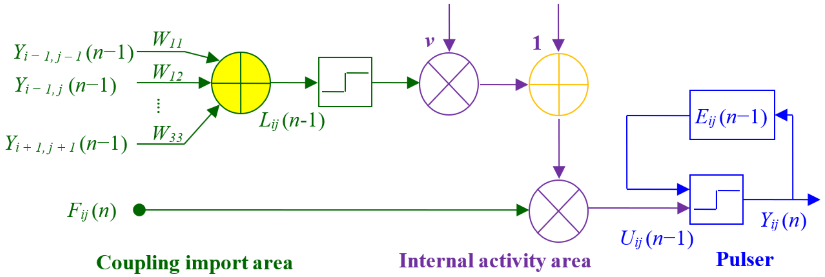
where nt is the number of iterations of the PCNN; i, j are image coordinates of one pixel; Yij is the pulse output; Wij is the connection coefficient in the coupling connection area; Lij is the connection input item; Fij is the input item of the neuron; and Uij is the internal activity item. Eij is the dynamic threshold, and v is the threshold extracted by the maximum inter-class variance algorithm (OTSU) that is used as the initial values of the parameters of the PCNN. The model of PCNN is shown in Figure A1 [37,38].
Figure A1.
Model of PCNN. The green part refers to the coupling import area, the purple one refers to the internal activity area, and the blue one refers to the pulser.
Figure A1.
Model of PCNN. The green part refers to the coupling import area, the purple one refers to the internal activity area, and the blue one refers to the pulser.

The link input items in the PCNN model were weighted. Before image segmentation, the threshold value was obtained based on the OTSU algorithm, and it was assigned to the link input weight, synaptic link coefficient, link weight amplification coefficient, and threshold iteration decay time constant in the improved model. The weighted processing of input link items can reduce the number of iterations and improve the real-time performance of the PCNN algorithm. On the basis of the OTSU algorithm, the network parameters of the improved PCNN model can be set adaptively.
- (2)
- Details about the comparison among edge extraction algorithms
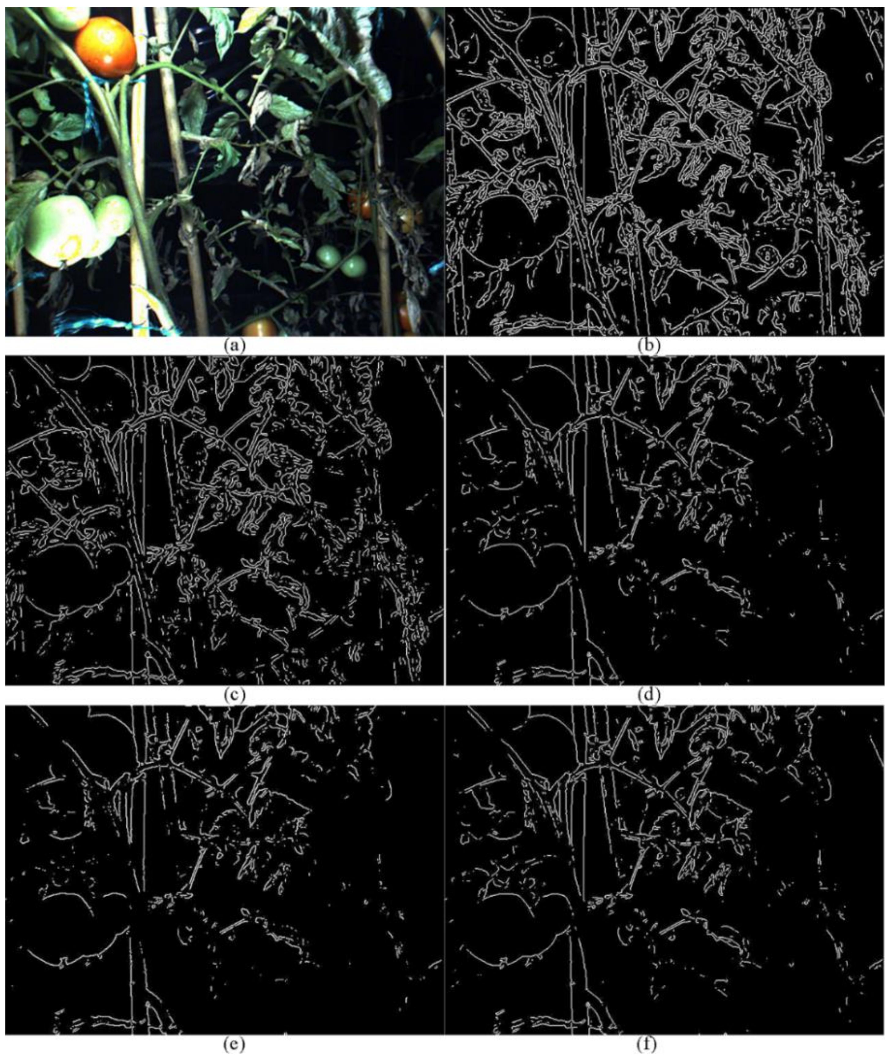
Several edge extraction algorithms (i.e., the Canny, Roberts, Sobel, Prewitt, and LOG operators) were tested to extract tomato plant edges. Figure A2 shows that the edge extracted by the Canny operator was the most complete amongst the other edges. Therefore, edges of tomato plants were extracted using the Canny algorithm. Figure A2c shows the edge extracted by the Canny operator of Figure A2a.
- (3)
- Details about edge sorting algorithm
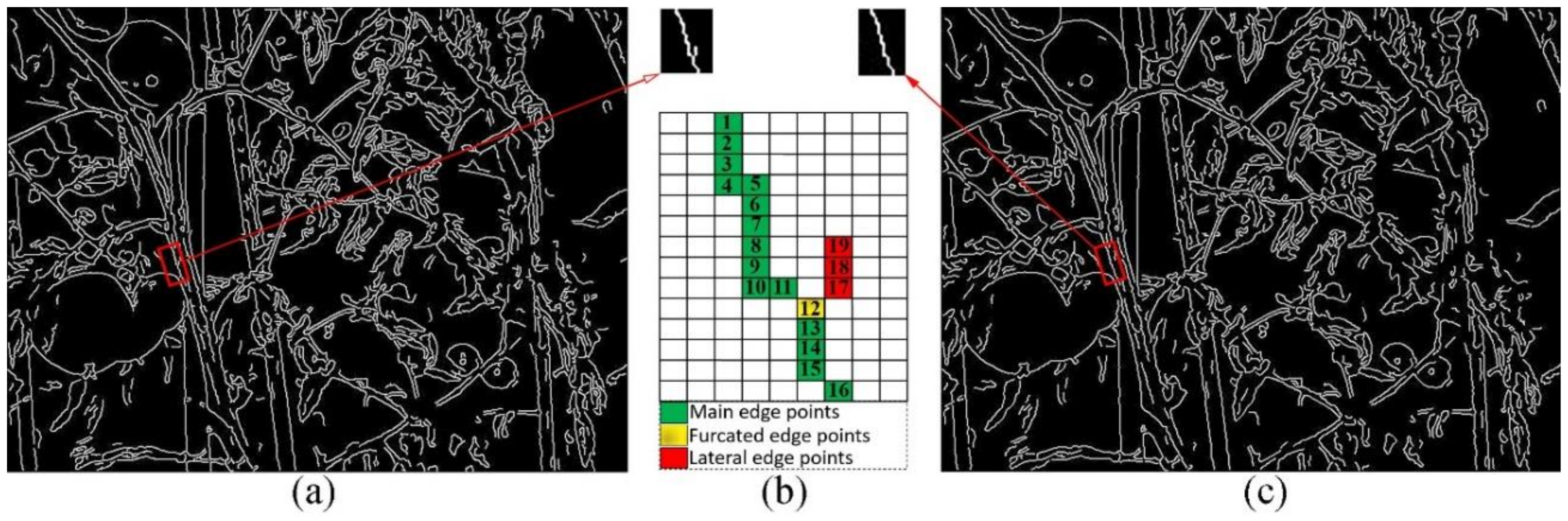
In Figure 5, the public edge refers to the edge that is shared by several longer edges. The recognition of fork points was based on the number and their position relationship with the edge points in eight neighbours of the current edge point. The current edge point is a fork point if there are only two edge points in eight neighbours of the current edge point and these two points are not one next to the other (i.e., the distance between these two points is larger than one pixel) or if the number of edge points in eight neighbours of the current edge point is larger than 3, which denotes there must be two points between which the distance is larger than one pixel. The edge composed of the fork point and sorted edge points before the fork point is the public edge. For example, the amplified local image in the red rectangle in Figure A3a is shown in Figure A3b. Points 1 to 11 are sorted points of the edge. Three points exist in the eight neighbours of point 12; thus, point 12 is a fork point, and the edge composed of points 1 to 12 is a public edge.
Figure A2.
Edges extracted by five operators: (a) raw image; (b) Canny operator; (c) LOG operator; (d) Prewitt operator; (e) Roberts operator; (f) Sobel operator.
Figure A2.
Edges extracted by five operators: (a) raw image; (b) Canny operator; (c) LOG operator; (d) Prewitt operator; (e) Roberts operator; (f) Sobel operator.

After edge sorting, several sorted edges exist for every continuous edge with fork points. The longest edge can be selected from edges that start from a same edge point to step over holes and edge burrs (noises) on sorted edges. Lateral edges are also extracted when public edges involved with the longest edge are removed from other edges. Short edges with lengths less than Tl are removed as noise. For instance, in Figure A3b, the length of the edge composed of points 1–12 and points 17–19 was less than that of the edge composed of points 1–16. Therefore, the edge composed of points 1–16 is the longest edge. The lateral edge is the edge composed of points 17–19, which comes from the edge composed of points 1–12 and points 17–19 after removing the public edge composed of points 1–12 and is involved with the longest edge. Given that the length of the lateral edge composed of points 17–19 is only three pixels and is less than Tl, this lateral edge is removed as noise [Figure A3c]. If we use traditional edge sorting based on neighbour pixels, this edge will be sorted into two edges: the edge composed of points 1–12 and points 17–19, and that composed of points 13–16. As a result, it increases the risk of false recognition of stem edges in later processing.
Figure A3.
Principle of the sorting algorithm: (a) Canny edges; (b) sorting principle; (c) sorted results.
Figure A3.
Principle of the sorting algorithm: (a) Canny edges; (b) sorting principle; (c) sorted results.

- (4)
- Details about edge type-labelling denoising algorithm
Many edge points remained that were not only up or down types in edge images of Eud but also left or right types in edge images of Elr acquired by Equation (1). To realise unique labelling for every edge point, a new edge type-labelling algorithm based on Tl neighbour denoising was designed. Traversing every point on a sorted edge in order, the number of every type of point in Tl neighbours of the current edge point in edge images Elr and Eud was counted. The Tl neighbours included Tl/2 pixels before and after the current edge point and the current edge point itself. The type of the current edge point was relabelled to the type with the largest number of points in its Tl neighbours. For the pixel in the first Tl/2 pixels of one sorted edge, its type was relabelled to the type with the largest number of points in the first Tl /2 pixels. Similarly, for the pixel in the last Tl/2 pixels of one sorted edge, its type was relabelled to the type with the largest number of points in the last Tl/2 pixels.
- (5)
- Several key points of stem duality edge extraction algorithmSeveral key points about stem duality edge extraction are presented as follows.
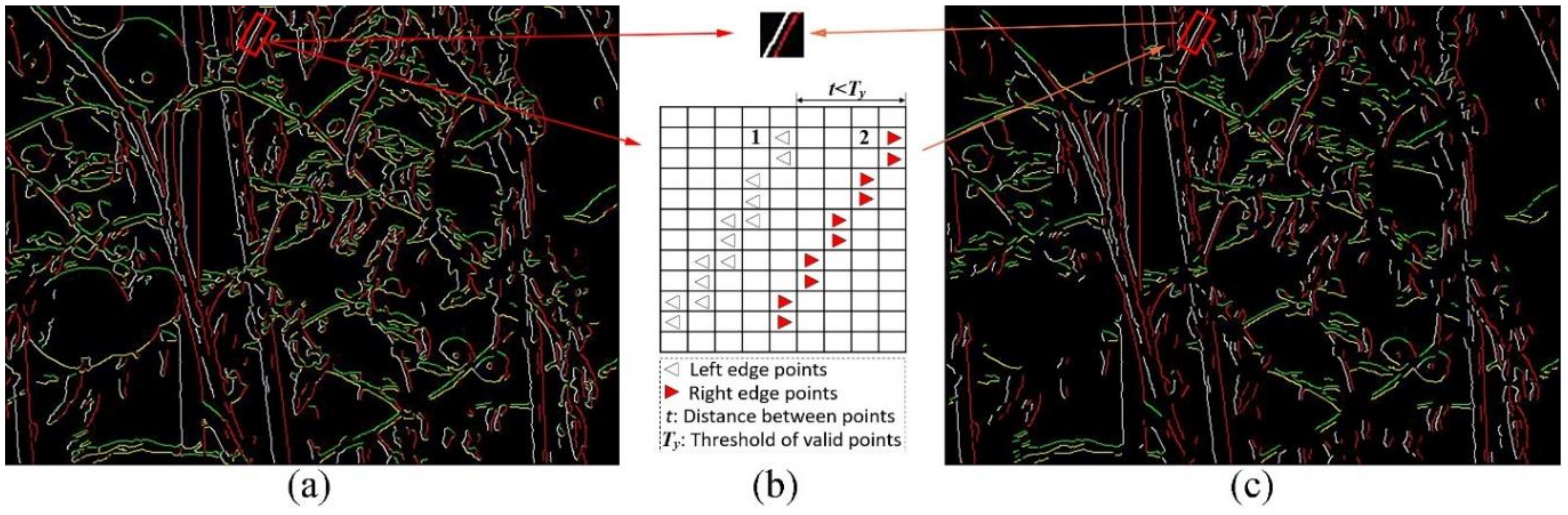
- In setting the scanning range for duality edges, the scanning range from YStart row to YEnd row and from XStart column to XEnd column was set based on the edge type of current edge point.If the edge type of current edge point is left, then YStart = y, YEnd = y, XStart = x + 1 and XEnd = x + Ts. For leaf edge pairs, the distance between one edge and its duality edge is smaller than 4Ty in images, so searching for the duality edge point in the range out of 4Ty pixels of one edge point is unnecessary. For this reason, Ts was set to 4Ty. The type of its duality edge point is right.If the edge type of the current edge point is right, then YStart = y, YEnd = y, XStart = x − 1 and XEnd = x − Ts. The type of its duality edge point is left.If the edge type of the current edge point is up, then YStart = y + 1, YEnd = y + Ts, XStart = x and XEnd = x. The type of its duality edge point is down.If the edge type of the current edge point is down, then YStart = y − 1, YEnd = y − Ts, XStart = x and XEnd = x. The type of its duality edge point is up.Figure A4b is the partial enlarged detail of the red rectangular region in Figure A4a. Taking point 1 in Figure A4b as an example, the edge type is left, and its image coordinate is (9, 274). Its scanning range for its duality edge point was set as YStart = 9, YEnd = 9, XStart = 275 and XEnd = 374, and the type of its duality edge point was right.
- In scanning for duality edge points and computing of the distance between current edge point and its duality edge point, we scanned the type of edge points on other edges from YStart row to YEnd row and from XStart column to XEnd column in the scanning range for one current edge point. The first edge point with the type of its duality edge point was its duality edge point. The distance t between the current edge point and its duality edge point was then computed. In Figure A4b, the distance t between point 1 and its duality edge point 2 with coordinate (9, 278) was 4.
- In recognition of valid duality edge points, if the distance t was smaller than the threshold Ty, this duality edge point was valid. In Figure A4b, the distance between point 1 and its duality point 2 was 4, which was smaller than Ty. Therefore, the edge point 2 was the valid duality edge point of point 1. The duality edge pair is in Figure A4c.
- In recognition of invalid duality edge points, if the distance t was larger than the threshold Ty, then this duality edge point was invalid.
- In recognition of invalid duality edges, if one duality edge had one or more invalid duality edge points, then this duality edge was invalid.
Figure A4.
Principle of stem duality edge extraction algorithm: (a) four type edges; (b) principle; (c) stem duality edges.
Figure A4.
Principle of stem duality edge extraction algorithm: (a) four type edges; (b) principle; (c) stem duality edges.

- (6)
- Details of the stem region recognition algorithm
The algorithm is as follows:
The mean distance between the dual edge point pair of stem edge pair was obtained. For stem edge point pairs, all pixels between the dual edge point pair were recognised as the pixels in stem regions. For stem edge points without dual edge point, pixels on the line starting from the stem edge point and extending along the dual direction (e.g., the dual direction of left type edge is the right side of the left edge point, and the dual direction of upper edge point is the underside of the upper edge point) were recognised as the pixels in the stem region. The length of the extending line was the mean distance between the dual edge point pair of stem edge pair. After all the stem edge pairs were treated above, the initial stem region identification result was obtained. The intersection of the initial stem region recognition result and the image segmentation result was obtained as the final stem region recognition result.
The list of parameters used in the study is shown in Table A1.

Table A1.
List of parameters used in the study.
| No. | Methods | Parameters | Values |
|---|---|---|---|
| 1 | DEM | Ty-threshold of the distance between left and right duality edge pairs used to recognise stems and leaves | 25/pixels |
| 2 | Tr-threshold of the length-width ratio of the minimum bounding rectangles of duality edges | 4.5 | |
| 3 | Mask R-CNN | initial learning rate of model training | 0.001 |
| 4 | momentum factor | 0.9 | |
| 5 | weight attenuation coefficient | 0.0001 | |
| 6 | step size of each iteration | 506 | |
| 7 | batch size | 2 | |
| 8 | anchor scale of RPN | 8, 16, 32, 64 and 128 |
Appendix B
Figure A5.
Model of Mask R-CNN.

References
- Arad, B.; Balendonck, J.; Barth, R.; Ben-Shahar, O.; Edan, Y.; Hellström, T.; Hemming, J.; Kurtser, P.; Ringdahl, O.; Tielen, T.; et al. Development of a sweet pepper harvesting robot. J. Field Robot. 2020, 37, 1027–1039. [Google Scholar] [CrossRef]
- McAllister, W.; Osipychev, D.; Davis, A.; Chowdhary, G. Agbots: Weeding a field with a team of autonomous robots. Comput. Electron. Agric. 2019, 163, 104827. [Google Scholar] [CrossRef]
- Wang, X.Z.; Han, X.; Mao, H.P. Vision-based detection of tomato main stem in greenhouse with red rope. Trans. Chin. Soc. Agric. Mach. 2012, 28, 135–141. [Google Scholar]
- Ota, T.; Bontsema, J.; Hayashi, S.; Kubota, K.; Van Henten, E.J.; Van Os, E.A.; Ajiki, K. Development of a cucumber leaf picking device for greenhouse production. Biosyst. Eng. 2007, 98, 381–390. [Google Scholar] [CrossRef]
- Van Henten, E.J.; Van Tuijl, B.A.J.; Hoogakker, G.J.; Van Der Weerd, M.J.; Hemming, J.; Kornet, J.G.; Bontsema, J. An Autonomous robot for de-leafing cucumber plants grown in a high-wire cultivation system. Biosyst. Eng. 2006, 94, 317–323. [Google Scholar] [CrossRef]
- Karkee, M.; Adhikari, B.; Amatya, S.; Zhang, Q. Identification of pruning branches in tall spindle apple trees for automated pruning. Comput. Electron. Agric. 2014, 103, 127–135. [Google Scholar] [CrossRef]
- Ma, B.J.; Du, J.; Wang, L.; Jiang, H.Y.; Zhou, M.C. Automatic branch detection of jujube trees based on 3D reconstruction for dormant pruning using the deep learning-based method. Comput. Electron. Agric. 2021, 190, 106484. [Google Scholar] [CrossRef]
- Sun, Q.X.; Chai, X.J.; Zeng, Z.K.; Zhou, G.M.; Sun, T. Multi-level feature fusion for fruit bearing branch keypoint detection. Comput. Electron. Agric. 2021, 191, 106479. [Google Scholar] [CrossRef]
- Kondo, N.; Yamamoto, K.; Yata, K.; Kurita, M. A machine vision for tomato cluster harvesting robot. In 2008 American Society of Agricultural and Biological Engineers Annual International Meeting; American Society of Agricultural and Biological Engineers: St. Joseph, MI, USA, 2008; p. 084044. [Google Scholar]
- Liang, C.X.; Xiong, J.T.; Zheng, Z.H.; Zhong, Z.; Li, Z.H.; Chen, S.M.; Yang, Z.G. A visual detection method for nighttime litchi fruits and fruiting stems. Comput. Electron. Agric. 2020, 169, 105192. [Google Scholar] [CrossRef]
- Xiong, J.T.; Lin, R.; Liu, Z.; He, Z.; Tang, L.Y.; Yang, Z.G.; Zou, X.J. The recognition of litchi clusters and the calculation of picking point in a nocturnal natural environment. Biosyst. Eng. 2018, 166, 44–57. [Google Scholar] [CrossRef]
- Zhong, Z.; Xiong, J.T.; Zheng, Z.H.; Liu, B.L.; Liao, S.S.; Huo, Z.W.; Yang, Z.G. A method for litchi picking points calculation in natural environment based on main fruit bearing branch detection. Comput. Electron. Agric. 2021, 189, 106398. [Google Scholar] [CrossRef]
- Colmenero-Martinez, J.T.; Blanco-Roldán, G.L.; Bayano-Tejero, S.; Castillo-Ruiz, F.J.; Sola-Guirado, R.R.; Gil-Ribes, J.A. An automatic trunk-detection system for intensive olive harvesting with trunk shaker. Biosyst. Eng. 2018, 172, 92–101. [Google Scholar] [CrossRef]
- Zhang, J.; He, L.; Karkee, M.; Zhang, Q.; Zhang, X.; Gao, Z.M. Branch detection for apple trees trained in fruiting wall architecture using depth features and Regions-Convolutional Neural Network (R-CNN). Comput. Electron. Agric. 2018, 155, 386–393. [Google Scholar] [CrossRef]
- Cai, J.R.; Sun, H.B.; Li, Y.P.; Sun, L.; Lu, H.Z. Fruit trees 3-D information perception and reconstruction based on binocular stereo vision. Trans. Chin. Soc. Agric. Mach. 2012, 43, 152–156. [Google Scholar]
- Van Henten, E.J.; Schenk, E.J.; Van Willigenburg, L.G.; Meuleman, J.; Barreiro, P. Collision-free inverse kinematics of the redundant seven-link manipulator used in a cucumber picking robot. Biosyst. Eng. 2010, 106, 112–124. [Google Scholar] [CrossRef] [Green Version]
- Chen, X.; Wang, S.; Zhang, B.; Luo, L. Multi-feature fusion tree trunk detection and orchard mobile robot localization using camera ultrasonic sensors. Comput. Electron. Agric. 2018, 147, 91–108. [Google Scholar] [CrossRef]
- Juman, M.A.; Wong, Y.W.; Rajkumar, R.K.; Goh, L.J. A novel tree trunk detection method for oil-palm plantation navigation. Comput. Electron. Agric. 2016, 128, 172–180. [Google Scholar] [CrossRef]
- Stefas, N.; Bayram, H.; Islera, V. Vision-based monitoring of orchards with UAVs. Comput. Electron. Agric. 2019, 163, 104814. [Google Scholar] [CrossRef]
- Amatya, S.; Karkee, M. Integration of visible branch sections and cherry clusters for detecting cherry tree branches in dense foliage canopies. Biosyst. Eng. 2016, 149, 72–81. [Google Scholar] [CrossRef] [Green Version]
- Ji, W.; Tao, Y.; Zhao, D.A.; Yang, J.; Ding, S.H. Iterative threshold segmentation of apple branch image based on CLAHE. Trans. Chin. Soc. Agric. Mach. 2014, 45, 69–75. [Google Scholar]
- Lu, Q.; Cai, J.R.; Liu, B.; Deng, L.; Zhang, Y.J. Identification of fruit and branch in natural scenes for citrus harvesting robot using machine vision and support vector machine. Int. J. Agric. Biol. Eng. 2014, 7, 115–121. [Google Scholar]
- Luo, L.F.; Zou, X.J.; Xiong, J.T.; Zhang, Y.; Peng, H.X.; Lin, G.H. Automatic positioning for picking point of grape picking robot in natural environment. Trans. Chin. Soc. Agric. Eng. 2015, 31, 14–21. [Google Scholar]
- Bac, C.W.; Hemming, J.; Van Henten, E.J. Robust pixel-based classification of obstacles for robotic harvesting of sweet-pepper. Comput. Electron. Agric. 2013, 96, 148–162. [Google Scholar] [CrossRef]
- Conto, T.D.; Olofsson, K.; Görgens, E.B.; EstravizRodriguez, L.C.; Almeida, G. Performance of stem denoising and stem modelling algorithms on single tree point clouds from terrestrial laser scanning. Comput. Electron. Agric. 2017, 143, 165–176. [Google Scholar] [CrossRef]
- Vázquez-Arellano, M.; Paraforos, D.S.; Reiser, D.; Garrido-Izard, M.; Griepentrog, H.W. Determination of stem position and height of reconstructed maize plants using a time-of-flight camera. Comput. Electron. Agric. 2018, 154, 276–288. [Google Scholar] [CrossRef]
- Nissimov, S.; Goldberger, J.; Alchanatis, V. Obstacle detection in a greenhouse environment using the Kinect sensor. Comput. Electron. Agric. 2015, 113, 104–115. [Google Scholar] [CrossRef]
- Amatya, S.; Karkee, M.; Gongal, A.; Zhang, Q.; Whiting, M.D. Detection of cherry tree branches with full foliage in planar architecture for automated sweet-cherry harvesting. Biosyst. Eng. 2016, 146, 3–15. [Google Scholar] [CrossRef] [Green Version]
- Bac, C.W.; Hemming, J.; Van Henten, E.J. Stem localization of sweet-pepper plants using the support wire as a visual cue. Comput. Electron. Agric. 2014, 105, 111–120. [Google Scholar] [CrossRef]
- Li, D.W.; Xu, L.H.; Tan, C.X.; Goodman, E.D.; Fu, D.C.; Xin, L.J. Digitization and visualization of greenhouse tomato plants in indoor environments. Sensors 2015, 15, 4019–4051. [Google Scholar] [CrossRef] [Green Version]
- Milella, A.; Marani, R.; Petitti, A.; Reina, G. In-field high throughput grapevine phenotyping with a consumer-grade depth camera. Comput. Electron. Agric. 2019, 156, 293–306. [Google Scholar] [CrossRef]
- Grimm, J.; Herzog, K.; Rist, F.; Kichere, A.; Topfer, R.; Steinhage, V. An adaptable approach to automated visual detection of plant organs with applications in grapevine breeding. Biosyst. Eng. 2019, 183, 170–183. [Google Scholar] [CrossRef]
- Jia, W.K.; Tian, Y.Y.; Luo, R.; Zhang, Z.H.; Lian, J.; Zheng, Y.J. Detection and segmentation of overlapped fruits based on optimized Mask R-CNN application in apple harvesting robot. Comput. Electron. Agric. 2020, 172, 105380. [Google Scholar] [CrossRef]
- Sun, J.; He, X.F.; Ge, X.; Wu, X.H.; Shen, J.F.; Song, Y.Y. Detection of key organs in tomato based on deep migration learning in a complex background. Agriculture 2019, 8, 196. [Google Scholar] [CrossRef] [Green Version]
- Zhong, W.Z.; Liu, X.L.; Yang, K.L.; Li, F.G. Research on multi-target leaf segmentation and recognition algorithm under complex background based on Mask-RCNN. Acta Agric. Zhejiangensis 2020, 32, 2059–2066. [Google Scholar]
- Eckhorn, R.; Reitboeck, H.J.; Arndt, M.; Dicke, P.W. Feature linking via synchronization among distributed assemblies: Simulations of results from cat visual cortex. Neural Comput. 1990, 2, 293–307. [Google Scholar] [CrossRef]
- Xiang, R. Image segmentation for whole tomato plant recognition at night. Comput. Electron. Agric. 2018, 154, 434–442. [Google Scholar] [CrossRef]
- Xiang, R.; Zhang, J.L. Image segmentation for tomato plants at night based on improved PCNN. Trans. Chin. Soc. Agric. Mach. 2020, 51, 130–137. [Google Scholar]
- Xiang, R.; Zhang, M.C. Tomato stem classification based on Mask R-CNN. J. Hunan Univ. (Nat. Sci.) 2022. submitted. [Google Scholar]
Figure 1.
Night lighting system and planting environment: (a) night lighting system; (b) planting environment.
Figure 1.
Night lighting system and planting environment: (a) night lighting system; (b) planting environment.

Figure 2.
Frame of the hybrid joint neural network.

Figure 3.
Flowchart of the method based on duality relation in edge pairs (DEM): (a) raw image; (b) binary image; (c) Canny edges; (d) sorted edges; (e) four type edges; (f) duality edges; (g) bounding rectangles; (h) stem edges; (i) result of the DEM. Red captions refer to the input and output images, and blue captions refer to images in process.

Figure 4.
Flowchart of edge sorting algorithm.

Figure 5.
Flowchart of stem duality edge extraction algorithm: (a) main flowchart; (b) sub-flowchart, processing of the current edge point. Color steps refer to core steps.
Figure 5.
Flowchart of stem duality edge extraction algorithm: (a) main flowchart; (b) sub-flowchart, processing of the current edge point. Color steps refer to core steps.

Figure 6.
Ground truth and its binary image: (a) ground truth of stems; (b) binary image of stem ground truth.
Figure 6.
Ground truth and its binary image: (a) ground truth of stems; (b) binary image of stem ground truth.

Figure 7.
Confusion matrices of test results of six methods: (a) DEM; (b) Mask R-CNN; (c) cascaded neural network composed of DEM and Mask R-CNN; (d) hybrid joint neural network; (e) YOLACT; (f) cascade neural network composed of DEM and YOLACT. Different colors represent different number of pixels, and darker colors represent more pixels.

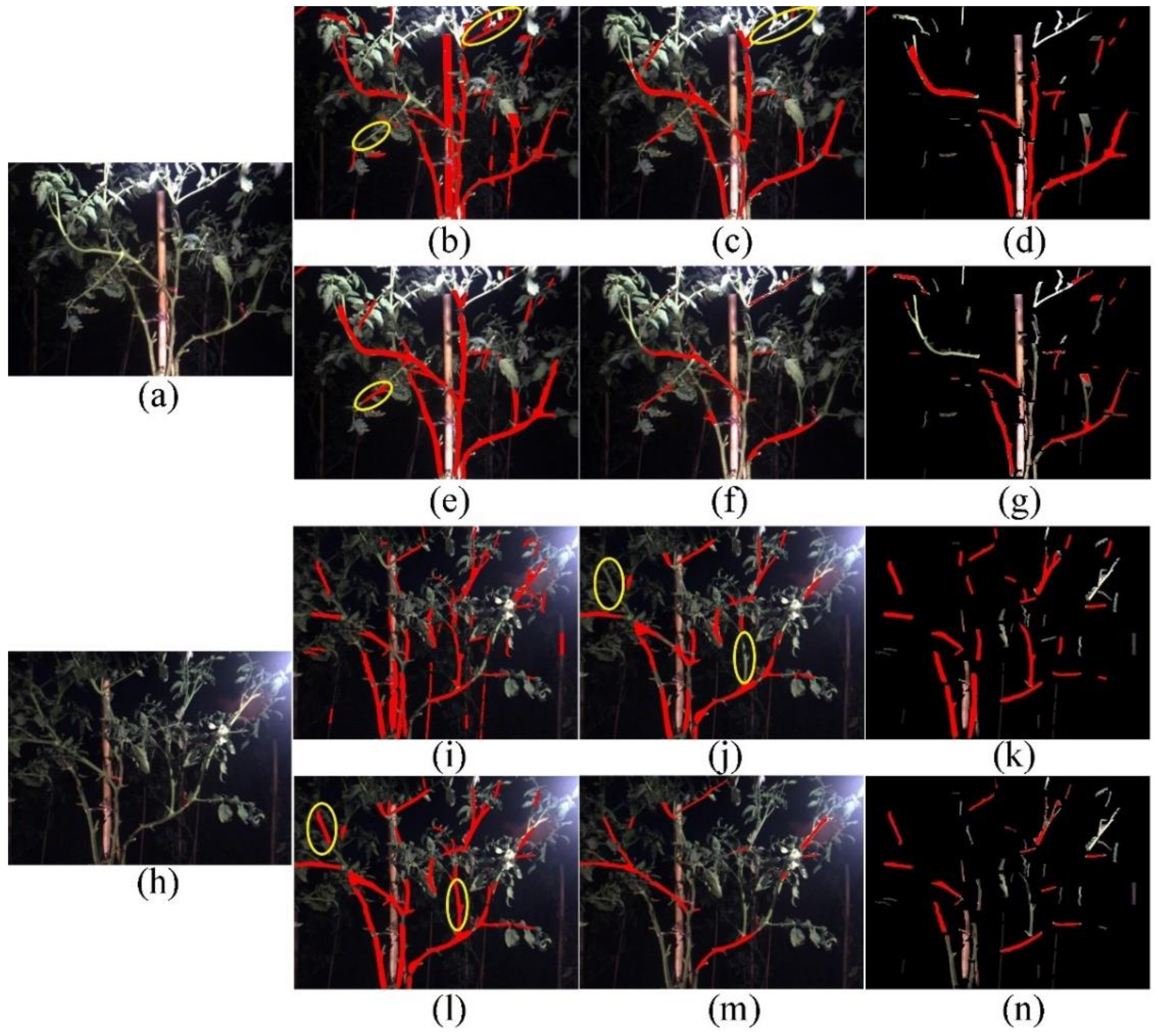
Figure 8.
Performance comparison among four algorithms: (a) raw image 1; (b) result 1 using DEM; (c) result 1 using Mask R-CNN; (d) result 1 using cascaded neural network composed of DEM and Mask R-CNN; (e) result 1 using hybrid joint neural network; (f) result 1 using YOLACT; (g) result 1 using cascaded neural network composed of DEM and YOLACT; (h) raw image 2; (i) result 2 using DEM; (j) result 2 using Mask R-CNN; (k) result 2 using cascaded neural network; (l) result 2 using hybrid joint neural network; (m) result 2 using YOLACT; (n) result 2 using cascaded neural network composed of DEM and YOLACT. Recognised results of stems in the yellow ellipses are different resulted from different methods. Through comparison, it shows the performance difference among different methods. The red regions represent the recognised stem regions.

Table 1.
Description of original and augmented datasets.
| Type | Dataset 1 | Dataset 2 | Total | ||
|---|---|---|---|---|---|
| Original dataset | 308 | 109 | 417 | ||
| Augmented dataset | Translation | Flip | Translation and flip | ||
| 289 | 327 | 288 | |||
| Training set Verification set | Testing set | ||||
| 1,012,200 | 109 | 1321 | |||
Table 2.
Metric values of test results of six methods.
| Lighting Conditions | (1) DEM | (2) Mask RCNN | ||||
| P% | R% | F1% | P% | R% | F1% | |
| 1st Condition 1 | 33.6 | 62.1 | 43.6 | 64.3 | 51.1 | 56.9 |
| 2nd Condition 2 | 32.0 | 54.5 | 40.3 | 69.2 | 48.6 | 57.0 |
| Total | 33.0 | 58.9 | 42.3 | 66.2 | 50.0 | 57.0 |
| Lighting Conditions | (3) Cascaded Neural Network (DEM + Mask RCNN) | (4) Hybrid Joint Neural Network | ||||
| P% | R% | F1% | P% | R% | F1% | |
| 1st Condition | 58.6 | 51.1 | 54.6 | 54.9 | 69.8 | 61.5 |
| 2nd Condition | 64.0 | 49.8 | 56.0 | 60.9 | 69.5 | 64.6 |
| Total | 60.7 | 50.5 | 55.2 | 57.2 | 69.7 | 62.8 |
| Lighting Conditions | (5) YOLACT | (6) Cascaded Neural Network (DEM + YOLACT) | ||||
| P% | R% | F1% | P% | R% | F1% | |
| 1st Condition | 78.8 | 25.6 | 38.6 | 68.4 | 21.7 | 33.0 |
| 2nd Condition | 82.6 | 36.9 | 51.0 | 71.3 | 23.6 | 35.4 |
| Total | 80.7 | 30.3 | 44.0 | 69.6 | 22.5 | 34.0 |
1 1st Condition: Two LEDs, 2 w, up and down layout. 2 2nd Condition: Two incandescent lamps, 15 w, opposite layout.
Publisher’s Note: MDPI stays neutral with regard to jurisdictional claims in published maps and institutional affiliations. |
© 2022 by the authors. Licensee MDPI, Basel, Switzerland. This article is an open access article distributed under the terms and conditions of the Creative Commons Attribution (CC BY) license (https://creativecommons.org/licenses/by/4.0/).
Share and Cite
MDPI and ACS Style
Xiang, R.; Zhang, M.; Zhang, J. Recognition for Stems of Tomato Plants at Night Based on a Hybrid Joint Neural Network. Agriculture 2022, 12, 743. https://0-doi-org.brum.beds.ac.uk/10.3390/agriculture12060743
AMA Style
Xiang R, Zhang M, Zhang J. Recognition for Stems of Tomato Plants at Night Based on a Hybrid Joint Neural Network. Agriculture. 2022; 12(6):743. https://0-doi-org.brum.beds.ac.uk/10.3390/agriculture12060743
Chicago/Turabian StyleXiang, Rong, Maochen Zhang, and Jielan Zhang. 2022. "Recognition for Stems of Tomato Plants at Night Based on a Hybrid Joint Neural Network" Agriculture 12, no. 6: 743. https://0-doi-org.brum.beds.ac.uk/10.3390/agriculture12060743
Note that from the first issue of 2016, this journal uses article numbers instead of page numbers. See further details here.