
An Improved EfficientNet for Rice Germ Integrity Classification and Recognition


College of Intelligent Systems Science and Engineering, Harbin Engineering University, Harbin 150001, China
*
Author to whom correspondence should be addressed.
Agriculture 2022, 12(6), 863; https://0-doi-org.brum.beds.ac.uk/10.3390/agriculture12060863
Submission received: 5 May 2022
/
Revised: 13 June 2022
/
Accepted: 14 June 2022
/
Published: 15 June 2022
(This article belongs to the Topic Emerging Agricultural Engineering Sciences, Technologies, and Applications)
Abstract
:Rice is one of the important staple foods for human beings. Germ integrity is an important indicator of rice processing accuracy. Traditional detection methods are time-consuming and highly subjective. In this paper, an EfficientNet–B3–DAN model is proposed to identify the germ integrity. Firstly, ten types of rice with different germ integrity are collected as the training set. Secondly, based on EfficientNet–B3, a dual attention network (DAN) is introduced to sum the outputs of two channels to change the representation of features and further focus on the extraction of features. Finally, the network is trained using transfer learning and tested on a test set. Comparing with AlexNet, VGG16, GoogleNet, ResNet50, MobileNet, and EfficientNet–B3, the experimental illustrate that the detection overall accuracy of EfficientNet–B3–DAN is 94.17%. It is higher than other models. This study can be used for the classification of rice germ integrity to provide guidance for rice and grain processing industries.
1. Introduction
Rice is a staple food for half of the world’s population. According to its size and shape, it is mainly divided into japonica and indica rice (Glaszmann, 1987) [1]. Germ-retaining rice has different definitions in different standards. In China’s “Retaining Germ Rice” Consultation Draft (Plan No.: 20142140-T-449), it is pointed out that germ-retaining rice is rice with a germ-retaining rate greater than 80%. Germ integrity refers to the proportion of germ to complete germ. The germ is an important part of rice, which contains 66% of the nutrients; therefore, accurate detection of germ integrity is of great practical value in guiding the rice milling equipment for accurate milling.
Earlier, the germ integrity was tested by manual methods, which were time consuming, unreliable, and subjective. For the grain processing industry, a fast, accurate, and objective testing method is urgently needed. Computer vision is widely used in agriculture as well as in rice quality inspection. It includes rice segmentation, rice counting, chalkiness detection, rice adulteration detection, etc. In terms of germ integrity detection, Xu [2] conducted research by analyzing the difference in appearance and area of rice with or without germ, and proposed a quadratic differential model to estimate the rice germ integrity information. Huang et al. [3] constructed a neural network model, including two neural networks and a selector, by analyzing the differences in the distinctive features of germinated rice and non-germinated rice. Through repeated training, the classification accuracy of germinated rice and non-germinated rice reached 93%. Huang et al. [4] converted RGB color gamut to HIV color gamut based on color features. In the HIV color gamut, the germ and endosperm have obvious differences in saturation, which is used as the basis for discriminating whether the germ is present or absent. The experiments showed that the method was close to the results of manual detection, with a similarity of 88%. In terms of fine rice yield detection, Yadav et al. [5] achieved the detection of polished rice yield by geometric features of rice grains. Yao et al. [6] completed the detection of milled rice yield by using concave point matching algorithm. In terms of rice quality detection, Duan et al. [7]; Liu et al. [8]; Sakai et al. [9]; Wan et al. [10]; Zareiforoush et al. [11] used the color and geometric features of images to detect rice quality. Lan et al. [12] used image enhancement technology to detect cracks in rice. Broken, chalky, speckled grains of rice were detected by Chen et al. [13] Sun et al. [14] used support vectors to classify plain and chalky rice. Sujarit et al. [15] used volume estimation to calculate the chalkiness of rice. With the rise of deep learning, researchers have used this method to study rice. Tan et al. [16] used convolutional neural networks to segment sticky rice grains. He et al. [17] used the method based on the background skeleton feature to complete the segmentation of sticky rice grains, and the segmentation accuracy reached 93.5%, which is better than the traditional watershed algorithm. Izquierdo et al. [18] built a convolutional neural network to classify different varieties of rice. Pradana-López et al. [19] uses transfer learning to detect rice adulteration.
In addition to the field of rice detection, researchers have also used deep learning to carry out a lot of research in other agricultural areas, which has promoted the development of agriculture. In terms of plant disease detection, Zhang et al. [20] used AlexNet [21] network to identify diseased leaves of cucumber. Gu et al. [22] used convolutional neural networks to identify apple and pear diseases. Atila et al. [23] used EfficientNet [24] to classify and detect plant leaf diseases. Tetile et al. [25] used ResNet [26] to detect and classify soybean pests in UAV images. Bi et al. [27] used the MoblieNet [28] network to identify apple leaf virus. In other agriculture, Yang et al. [29] used VGG [30] network to retrieve vegetable images. Gao et al. [31] used long short-term memory to predict soil moisture. Huang et al. [32] built their own convolutional neural network to achieve the classification of pineapple quality. Liu et al. [33,34] used an optimized neural network to identify spectral peaks and initially determine target locations. Yuan et al. [35] used the Inception-v2 [36] network to detect cherries and tomatoes.
In summary, a lot of research has been conducted on rice quality testing; however, there are few studies on the accurate detection of rice germ integrity. Germ integrity is a key indicator of rice, and the processing accuracy and nutritional composition of rice are closely related to it; therefore, it is of great significance to study the accurate detection method of rice germ integrity. In this paper, an EfficientNet–B3–DAN model is proposed to achieve rapid and accurate detection of germ integrity. The implementation steps are as follows: (1) On the basis of EfficientNet–B3, parallel attention modules are added, which are the position attention module (PAM) and the channel attention module (CAM). The PAM is able to learn the spatial interdependence of features and CAM can simulate the interdependence of channels to further improve the detection accuracy. (2) Several pictures of rice were collected and divided into 10 categories according to the germ integrity. (3) The model was trained by using the transfer learning method. Transfer learning can effectively save training time and improve detection accuracy with the help of features learned on other datasets.
2. Materials and Methods
This chapter introduces several rice samples used in the experiments and the deep learning models used to classify them.
2.1. Rice Varieties
In this paper, six varieties of rice were selected as experimental subjects, including four types of japonica rice and two types of indica rice. Their size and origin information are shown in Table 1.
2.2. Image Acquisition System
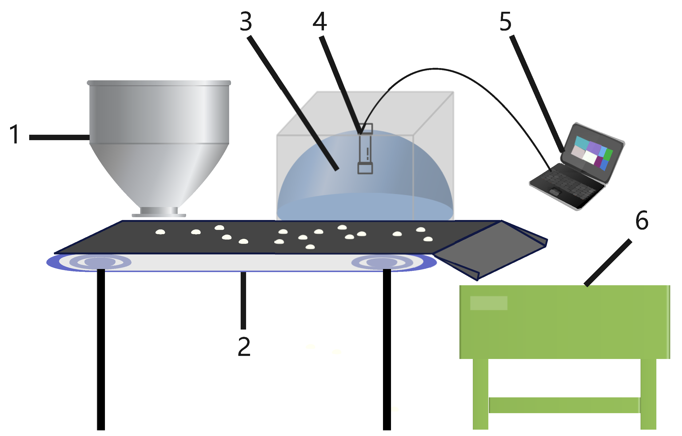
The image acpture system includes a Hikvision camera with 8 million pixels, a rice conveyor, an arched light source, and a computer, as shown in Figure 1.
The Hikvision camera is installed inside the arched light source to capture the rice on the transfer device vertically downward. A ring of LED lights is installed inside the arched light source to ensure a uniform distribution of light. In order to obtain a clear image, the brightness of the light source can be adjusted. The rice is randomly dropped on the conveyor device, which rotates at a constant speed. The camera captured images every 10 s, and the captured images were shown in the Figure 2. The processor of the notebook is 2.9 GHz, AMD Ryzen 7 4800 H. The operating system is Ubuntu18.04 64-bit operating system. QT Creator software is used as an image processing tool.
2.3. Image Preprocessing
In order to ensure the accuracy of the experiment, the rice was collected during the processing of the equipment. The collected images are densely stuck and cannot be trained directly. Preprocessing operations, such as region segmentation and sticky rice segmentation, are required.
2.3.1. Region Segmentation
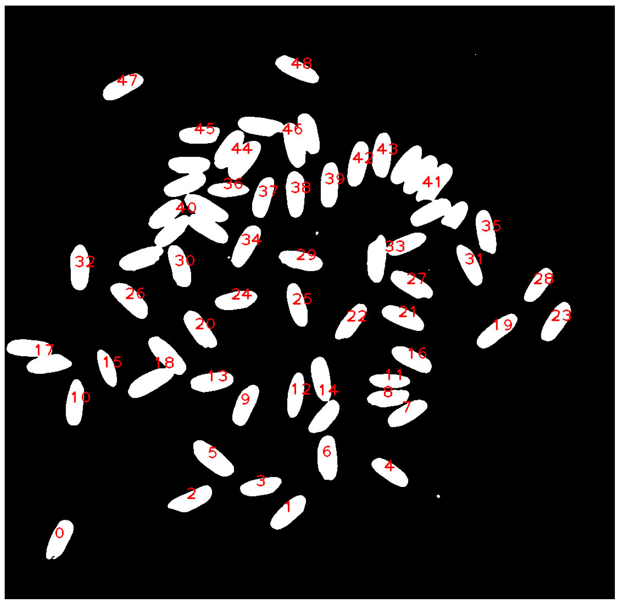
Region segmentation is to divide the image into several regions according to the similarity between pixels and surrounding pixels. Next, the rice binary image is segmented by the region growing method to complete the labeling and feature description of the region. The steps of the region growing method are as follows, first randomly designate a point in an area as the starting pixel, and continue to expand around this point. At the same time, determine the similarity between the surrounding pixels and this point, and if they are similar, add the surrounding pixels to the neighborhood. Secondly, continue to expand with the newly added point as the starting pixel point until there are no similar pixels around. Finally, an independent connected region is formed. The segmented graph is shown in the Figure 3.
2.3.2. Sticky Rice Segmentation
As shown in Figure 3, some marked areas contain multiple grains of rice, which need to be segmented. In this paper, an improved adaptive radius circular template method [16] is used, by which the concave points of rice in various adhesion cases can be found precisely. Then, the concave points are matched by the concave matching criterion, and finally the segmentation is completed. The specific steps are as follows:
- (1)
- According to the area size of the region, the adherent rice region was extracted as shown in the Figure 4.
- (2)
- The contours of the regions near the sticky rice are extracted. The corner response values along the boundary are calculated using the adaptive circular template. The calculation formula is as shown in Equation (1).
- (3)
- The segmentation endpoint is the concave point, which is screened according to the threshold value.
- (4)
- A concave point is randomly selected as the base endpoint, and possible matching points are found within the area formed by the specified angle. If there are multiple points, the closest matching point is selected as the matching point. If not, the base endpoint is changed to something else. Loop until all points are matched. At this point, the segmentation is completed. The segmentation result is shown in Figure 6.
2.4. EfficientNet–B3–DAN
EfficientNets is a network series published by Google in May 2019. They designed a baseline network using neural architecture search, and scaled the model to obtain a series of models. Its accuracy and efficiency are better than all previous convolutional networks. In particular, EfficientNet–B7 achieved a state-of-the-art top-1 accuracy of 84.4% on ImageNet, while being 8.4 times smaller and 6.1 times faster than the previous best convolutional network. After weighing the speed and accuracy, we chose the EfficientNet–B3 structure and improved on it.
2.4.1. The Structure of the EfficientNet–B3
2.4.2. Dual Attention Network (DAN)
The attention mechanism can exclude the interference of irrelevant information and pay more attention to useful information. DAN was proposed by Fu et al. [39]. The method can adaptively adjust the relationship between local features and global features, and achieve high accuracy in image segmentation. It includes a PAM and a CAM, which will catch rich contextual relations. Its structure is shown in Figure 7c.
2.5. Transfer Learning
Transfer learning is a technique in machine learning that applies data features and model parameters obtained in one dataset to another task, since training deep networks requires a lot of time and computational resources, and data collection also takes a lot of time. By transfer learning, we can not only save time but also achieve better classification accuracy. Our strategy is to use the weights trained on ImageNet. The ImageNet pre-trained model output is 1000-dimensional, which is changed to 10-dimensional according to our experimental needs. After experiments, it was found that the accuracy of training only the parameters of the fully connected layer was lower than that of training all the parameters; therefore, instead of freezing some parameters during training, all parameters were trained.
2.6. Experimental Setup
The experimental computer was configured as Inter(R) Core(TM) i7-6850K, the were 2 graphics cards, both 1080 ti. The Ubuntu18.04 operating system was installed, and the PyTorch framework was used for programming. The GPU environment was used for all experiments.
The input image size of the network is set to , and the epoch is set to 50. The base learning rate and batch size are set to and 32. Image operations such as horizontal flipping during training are used as image augmentation methods.
2.7. Evaluation Metrics
In the experiment of this paper, the performance of the model is comprehensively evaluated through five indicators. They are precision (Pre), sensitivity (Sen), accuracy (Acc), overall accuracy (OA), and F1-Score. The corresponding metrics of multi-categorization are calculated by using macro-averaging method. The formulas for these indicators are as follows:
The above indicators can be calculated by the confusion matrix. Among them, TP (True Positive), denotes that both label and output are positive. FP (False Positive), means that the label is positive, and the output is negative. TN (True Negative), means that both label and output are negative. FN (False Negative), which means the label is negative and the output is positive. M indicates how many categories. means how many correct predictions for each class, and N represents the sum of all samples.
3. Results and Discussion
3.1. Construction of Rice Dataset
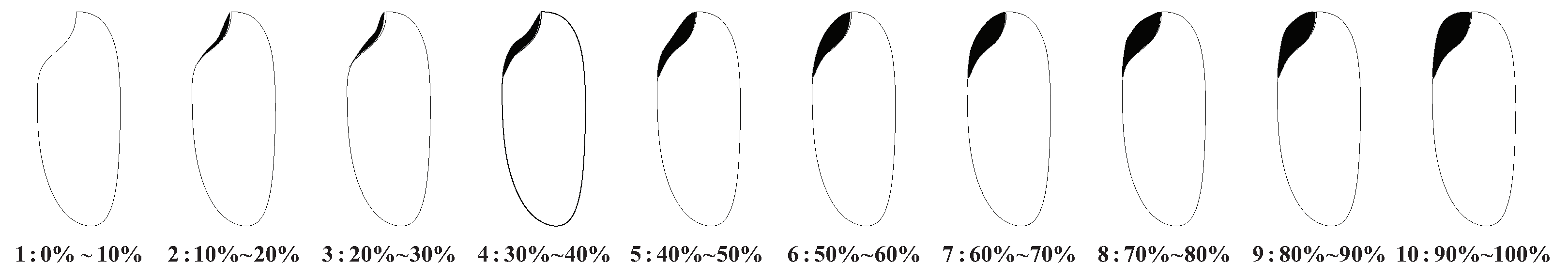
Through image preprocessing in Section 2.3, 10,392 single-grain rice images were obtained, which were divided into 10 categories according to different germ integrity, as shown in Figure 9.
Each type of rice is divided into training set, validation set, and test set according to the ratio of 60%, 20%, and 20%, as shown in Table 2. The training set serves to fit the network. The validation set tunes the model hyperparameters while saving the best weights. The role of the test set is to test the network performance.
3.2. Testing of the Model
3.2.1. Test Results of the EfficientNet–B3–DAN Model
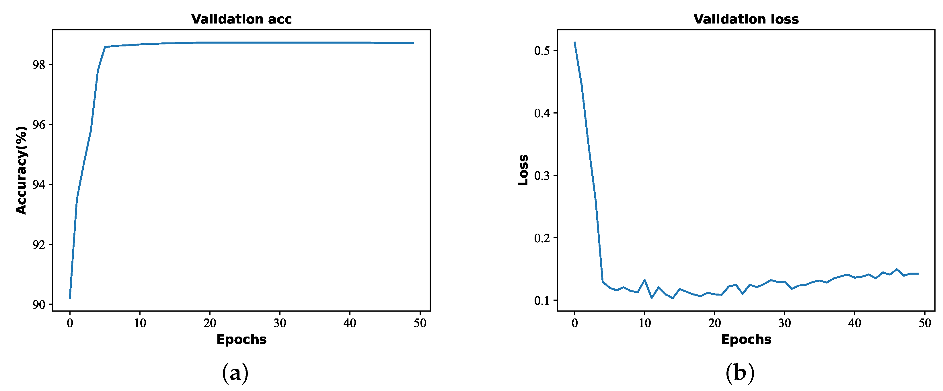
During the training process, the validation accuracy and validation loss data of the model at each epoch were obtained. As shown in Figure 10.
As shown in Figure 10, the accuracy and loss on the validation set reached stability in 5 epochs, with the highest average accuracy reaching 98.72% and the lowest loss reaching 0.1. The results show that the network can converge quickly and achieve high classification accuracy on the validation set.
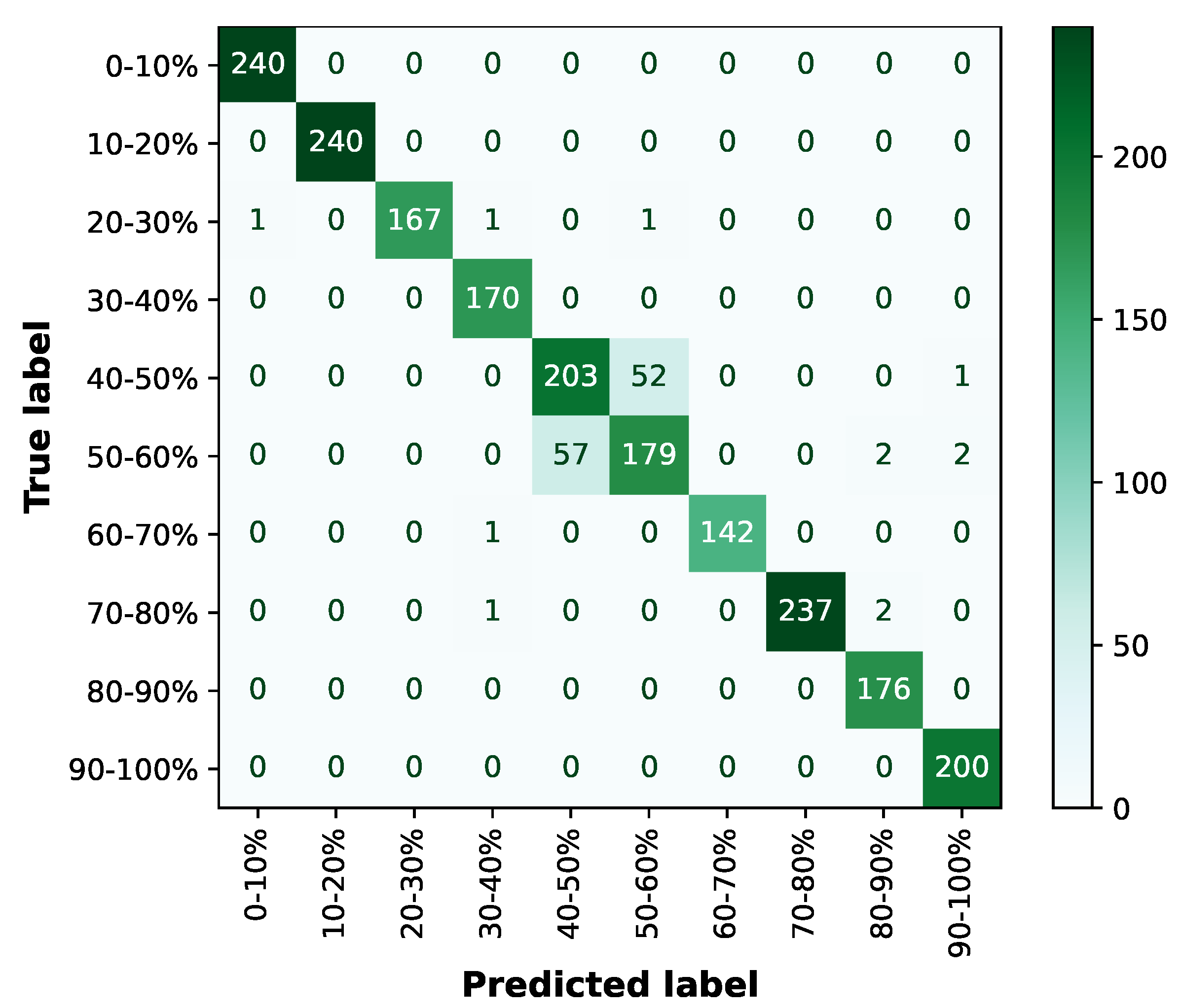
The test set was used to test the EfficientNet–B3–DAN. Figure 11 depicts the confusion matrix.
As can be seen from the confusion matrix, the numbers in the diagonal direction represent the number of correct classifications. The color blocks in the diagonal direction are darker, and the rest are lighter, indicating that most of the samples are correctly classified. The evaluation indexes are calculated according to the confusion matrix as shown in Table 3.
As can be seen from Table 3, the classification accuracy for each category is greater than 77.16%, the sensitivity is greater than 74.58%, and the accuracy is greater than 94.51%. Among them, the highest accuracy of the second category reaches 100%. In general, the model classification overall accuracy is 94.17%. In conclusion, the model is able to accurately classify the germ integrity dataset.
3.2.2. Compare Results with Other Methods
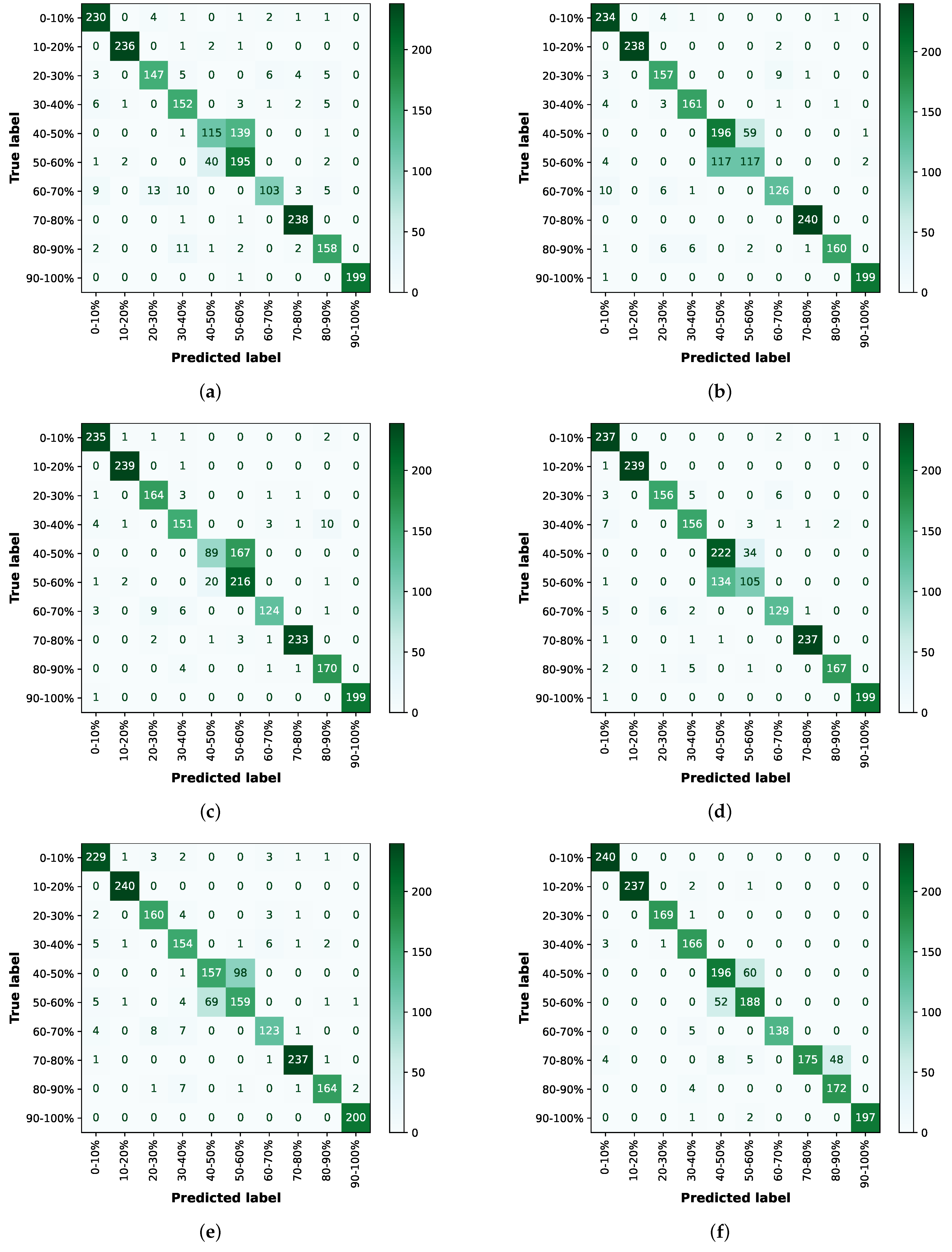
To further evaluate the detection performance of the proposed model, it is compared with other state-of-the-art models on the test set. Their confusion matrix is shown in Figure 12.
The data of several models on each indicators were obtained based on the confusion matrix calculation. As shown in Table 4.
Referring the Table 4, the EfficientNet–B3–DAN has a classification overall accuracy of 94.71% on the rice germ integrity test set, which is the best among several algorithms. It is higher than AlexNet, VGG16, ResNet50, GoogleNet, MobileNet, and EfficientNet–B3 by 8.72%, 6.07%, 6.46%, 5.16%, 6.31%, and 3.66%, respectively. The average accuracy, average sensitivity, and average precision are 3.19%, 3.38%, 0.74%, and 3.62% higher than the second place, respectively. The second place is EfficientNet–B3, therefore, it is reasonable to improve on it. After adding the DAN, the model has been improved in all indicators. It indicates that the DAN can establish rich contextual relationships on local features and effectively improve the classification accuracy.
In summary, our proposed EfficientNet–B3–DAN model can accurately classify germ integrity. Compared with other models, it has significant advantages in most of the indicators.
3.2.3. Visual Analysis
In order to better analyze the reasons why the EfficientNet–B3–DAN model outperforms other models, this paper uses the Grad-CAM [40] method for visualizing the classification results. Three kinds of rice were selected for the experiment. The attentional heat map is shown in Figure 13.
As shown in Figure 13, EfficientNet–B3 focuses on the germ region and part of the epidermal region of rice, while EfficientNet–B3–DAN focuses more on the rice germ region. The residual epidermis of rice is more similar to the germ region, which is easy to form interference. After adding the DAN, the model focuses more on the extraction of features in the germ region and enhances the representation of features, thus improving the classification accuracy of rice germ integrity. The feasibility of our proposed model is further proved through visualization.
4. Conclusions
Rice germ contains 66% of the important nutrients in rice; however, it is usually not retained during processing, resulting in serious food waste and affecting food security. In this paper, the EfficientNet–B3–DAN model is proposed to detect and classify the rice germ integrity to further guide the grain processing process. The overall accuracy of the EfficientNet–B3–DAN model reached 94.17% on the rice test set. Compared with other models, it has obvious advantages in various indicators. Through attentional heat map analysis, the EfficientNet–B3–DAN model can focus more on the extraction of germ part features, improve the feature expression capability, and further improve the classification accuracy.
This study can be applied to the grain processing industry to form a feedback system to improve grain production. In the follow-up work, we will continue to expand the data set of retained germ rice to achieve finer classification results. At the same time, it is necessary to further improve the detection accuracy and detection speed.
Moreover, our method can also be applied in the field of small object detection and classification. For example: cells, widgets, and other cereal categories. This is also our future research direction, combining with different disciplines, constantly exploring new methods and solving problems in different fields.
Author Contributions
Methodology, B.L. (Bing Li), B.L. (Bin Liu), S.L. and H.L.; validation, B.L. (Bin Liu), S.L. and H.L.; writing—original draft preparation, B.L. (Bin Liu) and H.L.; writing—review and editing, B.L. (Bing Li), B.L. (Bin Liu) and S.L; supervision, B.L. (Bing Li) and B.L. (Bin Liu). All authors have read and agreed to the published version of the manuscript.
Funding
This research was funded by the Natural Science Foundation of Heilongjiang Province grant number KY10400210217, Fundamental Strengthening Program Technical Field Fund grant number 2021-JCJQ-JJ-0026.
Institutional Review Board Statement
Not applicable.
Informed Consent Statement
Not applicable.
Data Availability Statement
Not applicable.
Conflicts of Interest
The authors declare no conflict of interest.
References
- Glaszmann, J.C. Isozymes and classification of Asian rice varieties. Theor. Appl. Genet. 1987, 74, 21–30. [Google Scholar] [CrossRef] [PubMed]
- Xu, L. Research on Measurement of Rice Plumule Ratio by Machine Vision. J. Jiangsu Univ. Sci. Technol. 1997, 6, 8–11. [Google Scholar]
- Huang, X.; Wu, S.; Fang, R. Research on Automatic Detection of Rice Embryo Retention Rate Using Neural Network Method. Trans. Chin. Soc. Agric. Eng. 1999, 4, 187–191. [Google Scholar]
- Huang, X.; Wu, S.; Fang, R.; Cai, J. Research on Application of Computer Vision in Identifying Rice Embryo. Trans. Chin. Soc. Agric. Mach. 2000, 31, 62–65. [Google Scholar]
- Yadav, B.K.; Jindal, V.K. Monitoring milling quality of rice by image analysis. Comput. Electron. Agric. 2001, 33, 19–33. [Google Scholar] [CrossRef]
- Yao, Y.; Wu, W.; Yang, T.; Liu, T.; Chen, W.; Chen, C.; Li, R.; Zhou, T.; Sun, C.; Zhou, Y.; et al. Head rice rate measurement based on concave point matching. Sci. Rep. 2017, 7, 41353. [Google Scholar] [CrossRef] [Green Version]
- Duan, L.; Yang, W.; Bi, K.; Chen, S.; Luo, Q.; Liu, Q. Fast discrimination and counting of filled/unfilled rice spikelets based on bi-modal imaging. Comput. Electron. Agric. 2011, 75, 196–203. [Google Scholar] [CrossRef]
- Liu, T.; Wu, W.; Chen, W.; Sun, C.; Chen, C.; Wang, R.; Zhu, X.; Guo, W. A shadow-based method to calculate the percentage of filled rice grains. Biosyst. Eng. 2016, 150, 79–88. [Google Scholar] [CrossRef]
- Sakai, N.; Yonekawa, S.; Matsuzaki, A.; Morishima, H. Two-dimensional image analysis of the shape of rice and its application to separating varieties. J. Food Eng. 1996, 27, 397–407. [Google Scholar] [CrossRef]
- Wan, P.; Long, C. An Inspection Method of Rice Milling Degree Based on Machine Vision and Gray-Gradient Co-occurrence Matrix. In Computer and Computing Technologies in Agriculture IV; Li, D., Liu, Y., Chen, Y., Eds.; Springer: Berlin/Heidelberg, Germany, 2011; pp. 195–202. [Google Scholar] [CrossRef] [Green Version]
- Zareiforoush, H.; Minaei, S.; Alizadeh, M.R.; Banakar, A. A hybrid intelligent approach based on computer vision and fuzzy logic for quality measurement of milled rice. Measurement 2015, 66, 26–34. [Google Scholar] [CrossRef]
- Lan, Y.; Fang, Q.; Kocher, M.F.; Hanna, M.A. Detection of Fissures in Rice Grains Using Imaging Enhancement. Int. J. Food Prop. 2002, 5, 205–215. [Google Scholar] [CrossRef] [Green Version]
- Chen, S.; Xiong, J.; Guo, W.; Bu, R.; Zheng, Z.; Chen, Y.; Yang, Z.; Lin, R. Colored rice quality inspection system using machine vision. J. Cereal Sci. 2019, 88, 87–95. [Google Scholar] [CrossRef]
- Sun, C.; Liu, T.; Ji, C.; Jiang, M.; Tian, T.; Guo, D.; Wang, L.; Chen, Y.; Liang, X. Evaluation and analysis the chalkiness of connected rice kernels based on image processing technology and support vector machine. J. Cereal Sci. 2014, 60, 426–432. [Google Scholar] [CrossRef]
- Sujarit, A.; Cheaupan, K.; Chattham, N. Detection of rice grain chalkiness level with volume estimation from image processing. Proc. SPIE 2020, 11331, 34. [Google Scholar] [CrossRef]
- Tan, S.; Ma, X.; Mai, Z.; Qi, L.; Wang, Y. Segmentation and counting algorithm for touching hybrid rice grains. Comput. Electron. Agric. 2019, 162, 493–504. [Google Scholar] [CrossRef]
- Li, B.; He, C. Segmentation algorithm of touching rice kernels based on skeleton features of image background. J. Comput. Appl. 2017, 37, 198–202. [Google Scholar]
- Izquierdo, M.; Lastra-Mejías, M.; González-Flores, E.; Pradana-López, S.; Cancilla, J.C.; Torrecilla, J.S. Visible imaging to convolutionally discern and authenticate varieties of rice and their derived flours. Food Control 2020, 110, 106971. [Google Scholar] [CrossRef]
- Pradana-López, S.; Pérez-Calabuig, A.M.; Rodrigo, C.; Lozano, M.A.; Cancilla, J.C.; Torrecilla, J.S. Low requirement imaging enables sensitive and robust rice adulteration quantification via transfer learning. Food Control 2021, 127, 108122. [Google Scholar] [CrossRef]
- Zhang, S.; Zhang, S.; Zhang, C.; Wang, X.; Shi, Y. Cucumber leaf disease identification with global pooling dilated convolutional neural network. Comput. Electron. Agric. 2019, 162, 422–430. [Google Scholar] [CrossRef]
- Krizhevsky, A.; Sutskever, I.; Hinton, G.E. ImageNet classification with deep convolutional neural networks. Commun. ACM 2017, 60, 84–90. [Google Scholar] [CrossRef]
- Gu, Y.H.; Yin, H.; Jin, D.; Zheng, R.; Yoo, S.J. Improved Multi-Plant Disease Recognition Method Using Deep Convolutional Neural Networks in Six Diseases of Apples and Pears. Agriculture 2022, 12, 300. [Google Scholar] [CrossRef]
- Atila, V.; Uçar, M.; Akyol, K.; Uçar, E. Plant leaf disease classification using EfficientNet deep learning model. Ecol. Informatics 2021, 61, 101182. [Google Scholar] [CrossRef]
- Tan, M.; Le, Q.V. EfficientNet: Rethinking Model Scaling for Convolutional Neural Networks. arXiv 2020, arXiv:1905.11946. [Google Scholar]
- Tetila, E.C.; Machado, B.B.; Astolfi, G.; Belete, N.A.d.S.; Amorim, W.P.; Roel, A.R.; Pistori, H. Detection and classification of soybean pests using deep learning with UAV images. Comput. Electron. Agric. 2020, 179, 105836. [Google Scholar] [CrossRef]
- He, K.; Zhang, X.; Ren, S.; Sun, J. Deep Residual Learning for Image Recognition. In Proceedings of the 2016 IEEE Conference on Computer Vision and Pattern Recognition (CVPR), Las Vegas, NV, USA, 27–30 June 2016; pp. 770–778. [Google Scholar] [CrossRef] [Green Version]
- Bi, C.; Wang, J.; Duan, Y.; Fu, B.; Kang, J.R.; Shi, Y. MobileNet Based Apple Leaf Diseases Identification. Mob. Netw. Appl. 2022, 27, 172–180. [Google Scholar] [CrossRef]
- Howard, A.G.; Zhu, M.; Chen, B.; Kalenichenko, D.; Wang, W.; Weyand, T.; Andreetto, M.; Adam, H. MobileNets: Efficient Convolutional Neural Networks for Mobile Vision Applications. arXiv 2017, arXiv:1704.04861. [Google Scholar]
- Yang, Z.; Yue, J.; Li, Z.; Zhu, L. Vegetable Image Retrieval with Fine-tuning VGG Model and Image Hash. IFAC-PapersOnLine 2018, 51, 280–285. [Google Scholar] [CrossRef]
- Simonyan, K.; Zisserman, A. Very Deep Convolutional Networks for Large-Scale Image Recognition. arXiv 2014, arXiv:1409.1556. [Google Scholar]
- Gao, P.; Qiu, H.; Lan, Y.; Wang, W.; Chen, W.; Han, X.; Lu, J. Modeling for the Prediction of Soil Moisture in Litchi Orchard with Deep Long Short-Term Memory. Agriculture 2022, 12, 25. [Google Scholar] [CrossRef]
- Huang, T.W.; Bhat, S.A.; Huang, N.F.; Chang, C.Y.; Chan, P.C.; Elepano, A.R. Artificial Intelligence-Based Real-Time Pineapple Quality Classification Using Acoustic Spectroscopy. Agriculture 2022, 12, 129. [Google Scholar] [CrossRef]
- Liu, H.; Xu, B.; Liu, B. An Automatic Search and Energy-Saving Continuous Tracking Algorithm for Underwater Targets Based on Prediction and Neural Network. J. Mar. Sci. Eng. 2022, 10, 283. [Google Scholar] [CrossRef]
- Liu, H.; Xu, B.; Liu, B. A Tracking Algorithm for Sparse and Dynamic Underwater Sensor Networks. J. Mar. Sci. Eng. 2022, 10, 337. [Google Scholar] [CrossRef]
- Yuan, T.; Lv, L.; Zhang, F.; Fu, J.; Gao, J.; Zhang, J.; Li, W.; Zhang, C.; Zhang, W. Robust Cherry Tomatoes Detection Algorithm in Greenhouse Scene Based on SSD. Agriculture 2020, 10, 160. [Google Scholar] [CrossRef]
- Szegedy, C.; Liu, W.; Jia, Y.; Sermanet, P.; Reed, S.; Anguelov, D.; Erhan, D.; Vanhoucke, V.; Rabinovich, A. Going Deeper with Convolutions. arXiv 2014, arXiv:1409.4842. [Google Scholar]
- Sandler, M.; Howard, A.; Zhu, M.; Zhmoginov, A.; Chen, L.C. MobileNetV2: Inverted Residuals and Linear Bottlenecks. arXiv 2018, arXiv:1801.04381. [Google Scholar]
- Hu, J.; Shen, L.; Albanie, S.; Sun, G.; Wu, E. Squeeze-and-Excitation Networks. arXiv 2019, arXiv:1709.01507. [Google Scholar]
- Fu, J.; Liu, J.; Tian, H.; Li, Y.; Bao, Y.; Fang, Z.; Lu, H. Dual Attention Network for Scene Segmentation. In Proceedings of the 2019 IEEE/CVF Conference on Computer Vision and Pattern Recognition (CVPR), Long Beach, CA, USA, 15–20 June 2019; pp. 3141–3149. [Google Scholar] [CrossRef] [Green Version]
- Selvaraju, R.R.; Cogswell, M.; Das, A.; Vedantam, R.; Parikh, D.; Batra, D. Grad-CAM: Visual Explanations from Deep Networks via Gradient-based Localization. Int. J. Comput. Vis. 2020, 128, 336–359. [Google Scholar] [CrossRef] [Green Version]
Figure 1.
Image acquisition system. 1. Hopper. 2. Transfer device. 3. Arched light source. 4. Hikvision camera. 5. Notebook. 6. Storage hopper. Working process: The rice is sprinkled on the conveyor belt by the feeding hopper. The conveyor belt advances at a constant speed, and the camera is controlled by the notebook to take pictures regularly. Finally the rice is collected by the storage hopper.

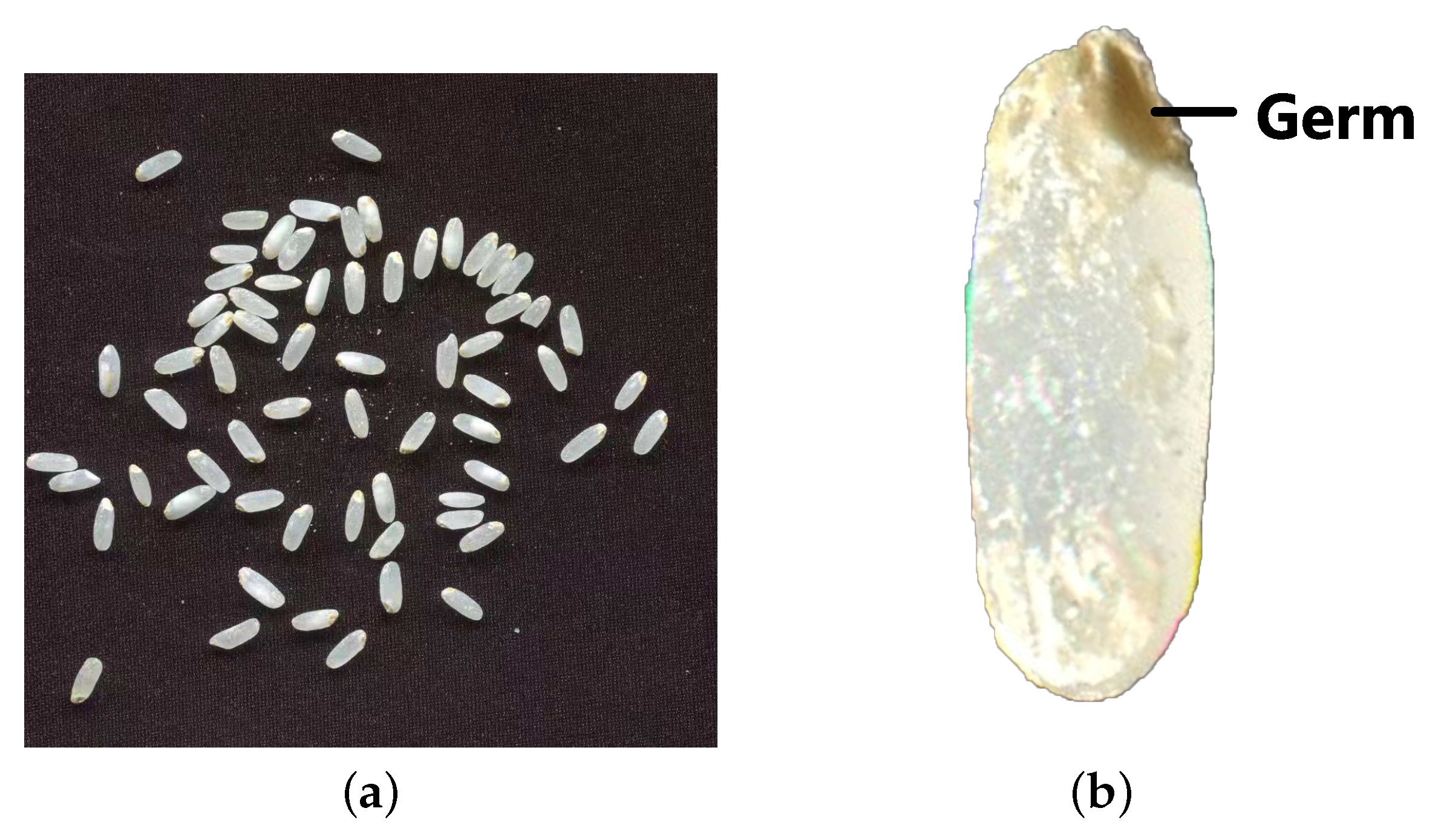
Figure 2.
Collected images. (a) Full image. (b) Single germ rice.

Figure 3.
Labeling results of region segmentation.

Figure 4.
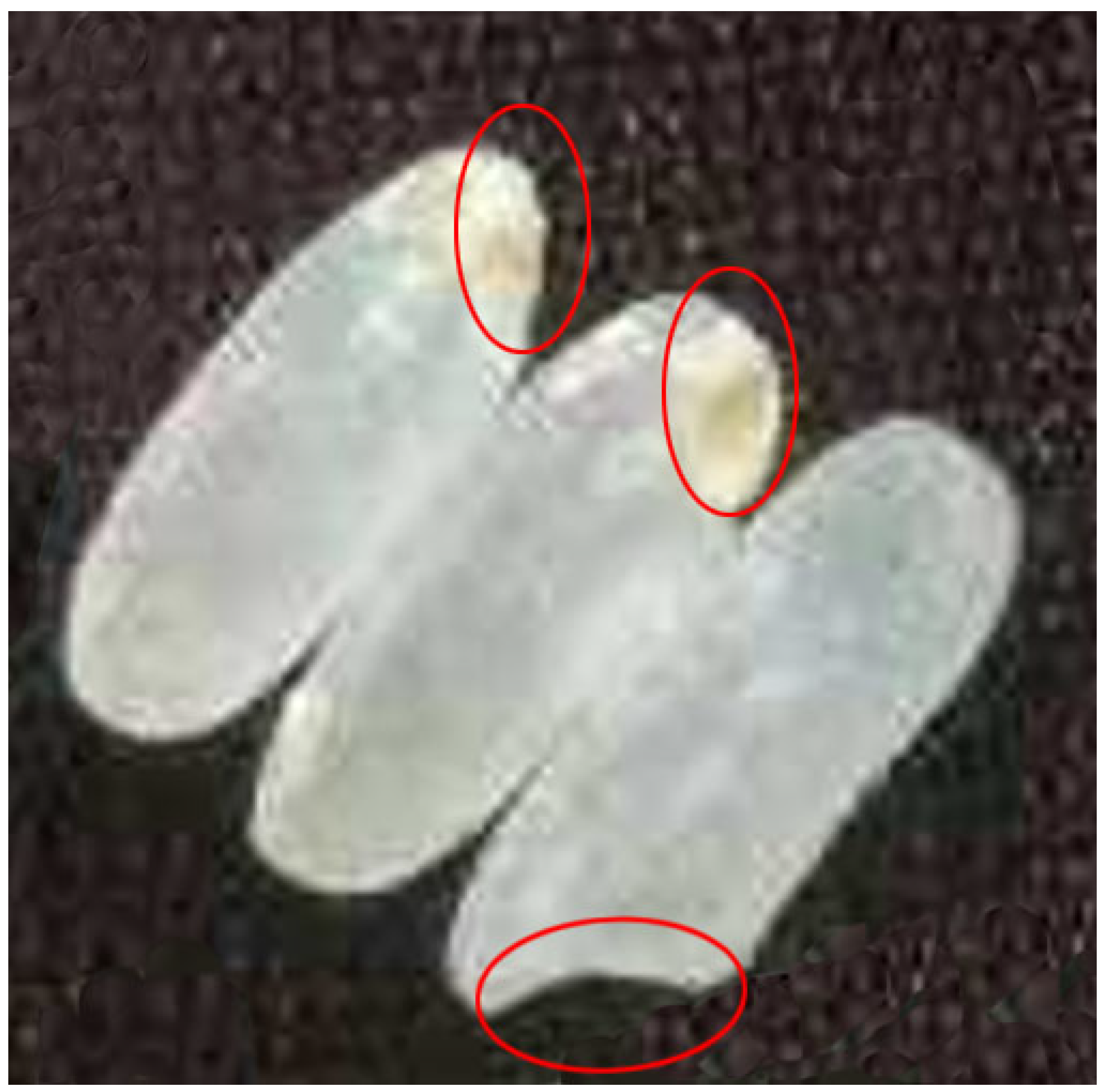
Image of rice seeds with various degree of germ integrity. The red oval indicates the position of the germ.
Figure 4.
Image of rice seeds with various degree of germ integrity. The red oval indicates the position of the germ.

Figure 5.
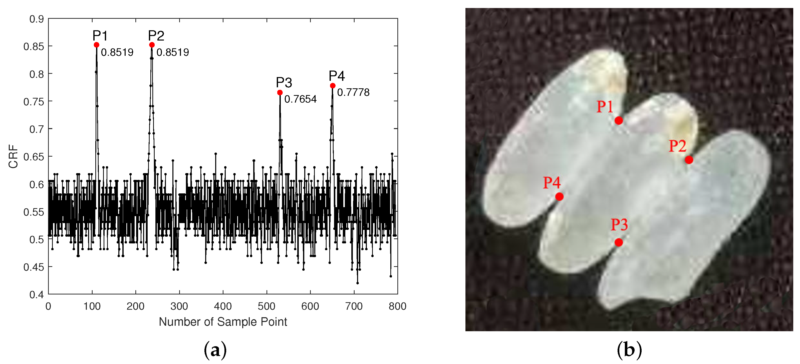
Corner response. Along the rice boundary, the CRF of each pixel is calculated. The response curve of the corner point is obtained, and the corresponding corner point in the image is found according to the local maximum point in the curve. (a) Corner response curve. (b) Corner points correspond to points on the image.
Figure 5.
Corner response. Along the rice boundary, the CRF of each pixel is calculated. The response curve of the corner point is obtained, and the corresponding corner point in the image is found according to the local maximum point in the curve. (a) Corner response curve. (b) Corner points correspond to points on the image.

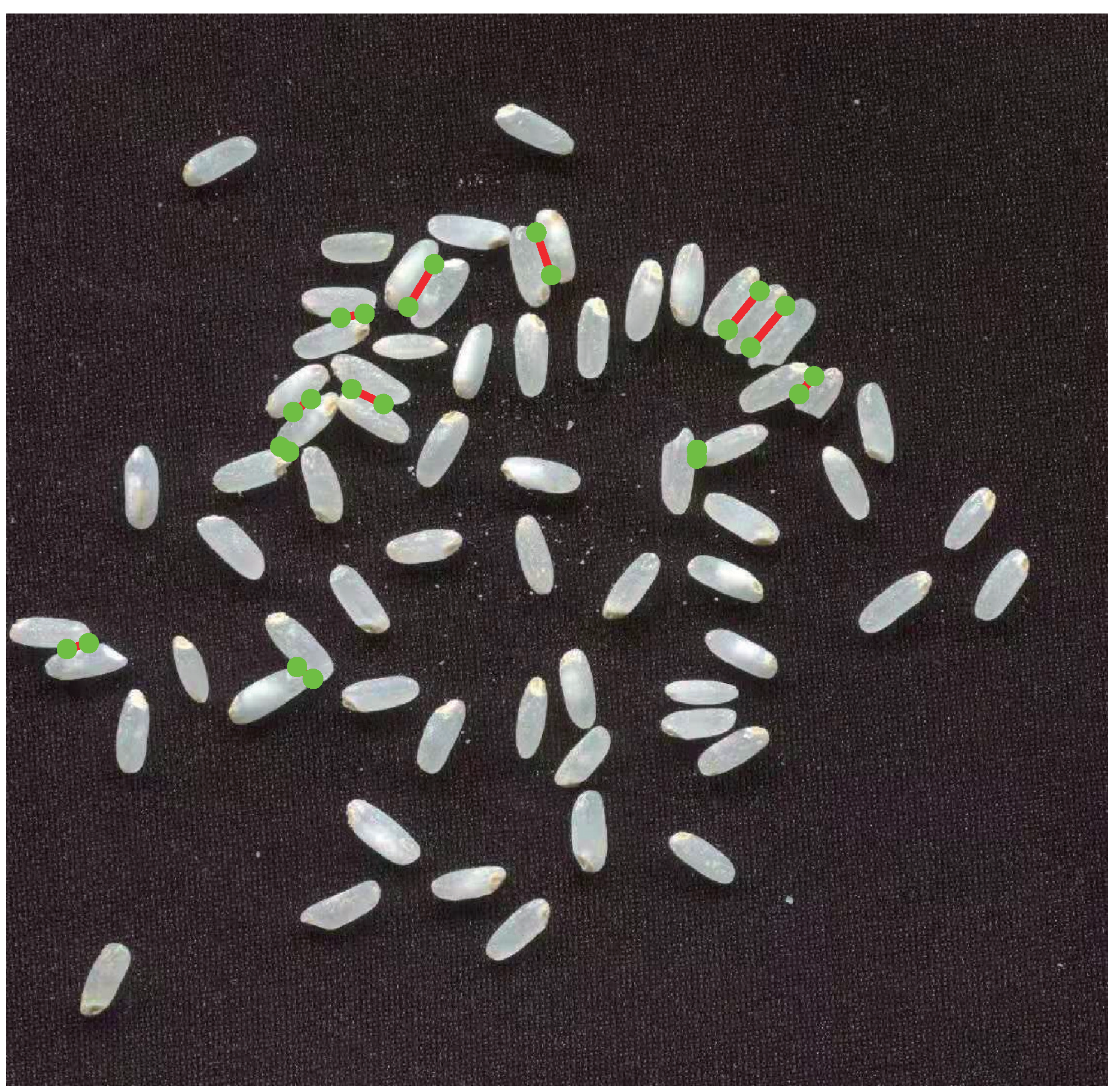
Figure 6.
Segmentation result.

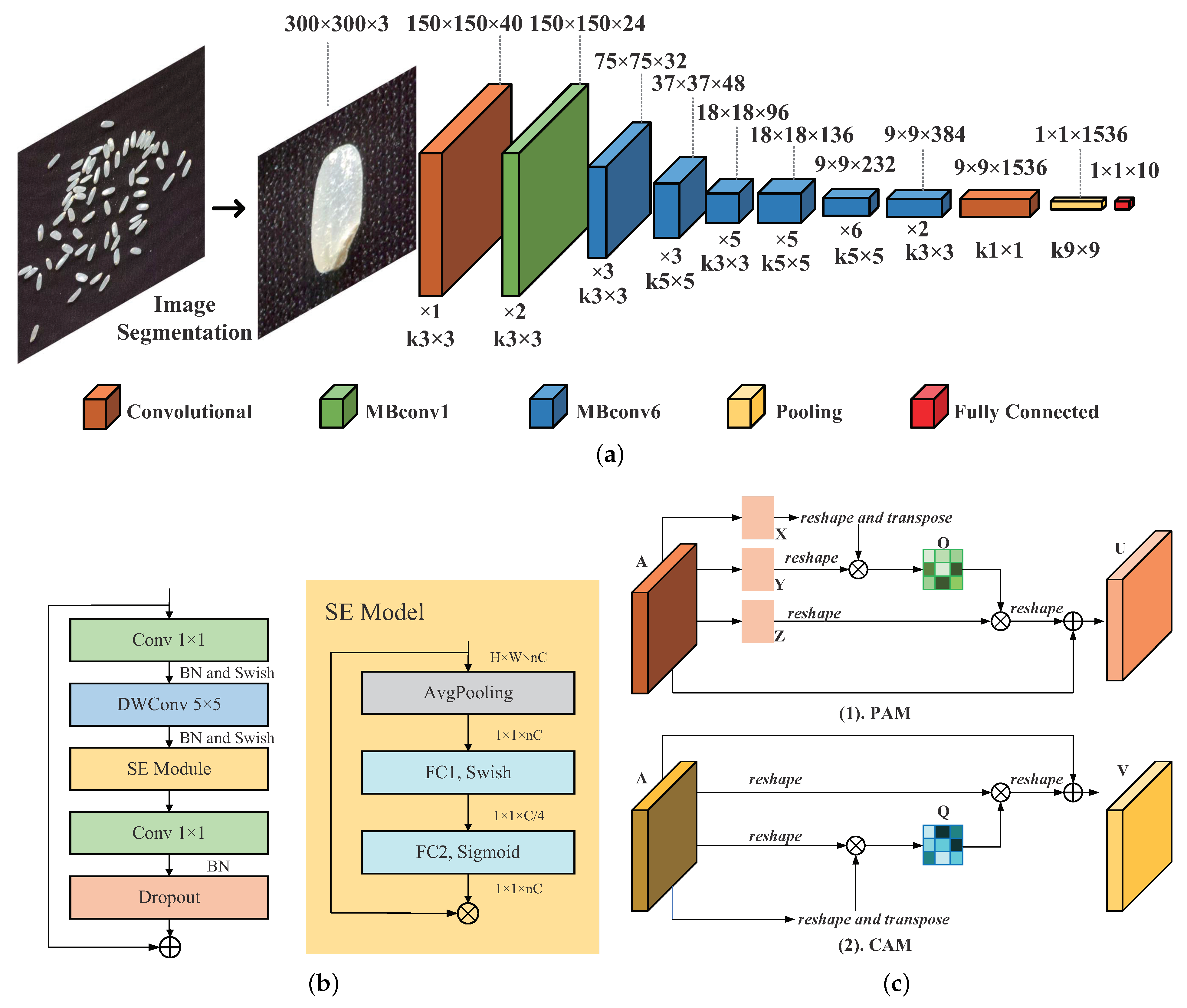
Figure 7.
The individual structures included in EfficientNet–B3–DAN. (a) The structure of the EfficientNet–B3. indicates that the layer is repeated n times, and indicates that the size of the convolution kernel is n. MBConv means mobile inverted bottleneck convolution, proposed by Sandler et al. [37]. The image input size is , and the final classification result is output through the convolutional layer, the MBconv1 layer, the MBConv6 layer, the pooling layer, and the fully connected layer. (b) On the left the is structure of the MBConv. Conv represents the convolutional layer, BN represents the batch normalization layer, Swish means the Swish activation function, DWConv means the deep separable convolution, and SE represents the squeeze-and-excitation [38]. The size of the input feature map is , and the dimension is expanded by n times through the convolutional layer. For example, Mbconv6 means to expand by six times. On the right is the structure of SE. AvgPooling denotes average pooling and FC denotes fully connected layer. Through this module, the dependencies between different channels can be adaptively learned. (c) The structure of DAN. The upper figure represents the PAM. Input feature map , the size is , and the feature map is convolved to obtain , , , and the size is still . Transform and into , , their size is , where . After that, is calculated. Compute the by softmax with size . Transform the size of to , multiply it with , and finally sum with to obtain the final output . The lower figure represents the CAM. The input feature map is still , transform into , the size is . is calculated. is output through the softmax layer, the magnitude of is . Multiply and , and the result size is transformed into . Finally, add to obtain . The PAM is summed with the CAM as the output of the dual attention network.

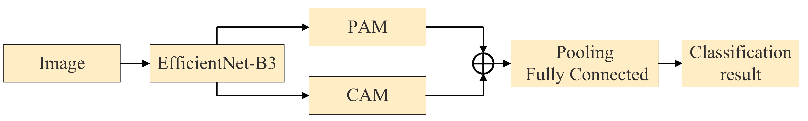
Figure 8.
The structure of the EfficientNet–B3–DAN.

Figure 9.
Ten kinds of rice with different germ integrity. The black area in the figure represents the rice germ part.
Figure 9.
Ten kinds of rice with different germ integrity. The black area in the figure represents the rice germ part.

Figure 10.
Data for each epoch. Accuracy and loss for each epoch on the validation set. (a) Validation accuracy. (b) Validation loss.
Figure 10.
Data for each epoch. Accuracy and loss for each epoch on the validation set. (a) Validation accuracy. (b) Validation loss.

Figure 11.
Confusion matrix of EfficientNet–B3–DAN. The horizontal axis represents the predicted labels for each category, and the vertical axis represents the true labels for each category. Each grid represents the number of classes predicted to be another class. The diagonal cells represent the number of correct predictions.

Figure 12.
Confusion matrix for different networks. (a) AlexNet. (b) VGG. (c) ResNet. (d) GoogleNet. (e) MobileNet. (f) EfficientNet–B3.
Figure 12.
Confusion matrix for different networks. (a) AlexNet. (b) VGG. (c) ResNet. (d) GoogleNet. (e) MobileNet. (f) EfficientNet–B3.

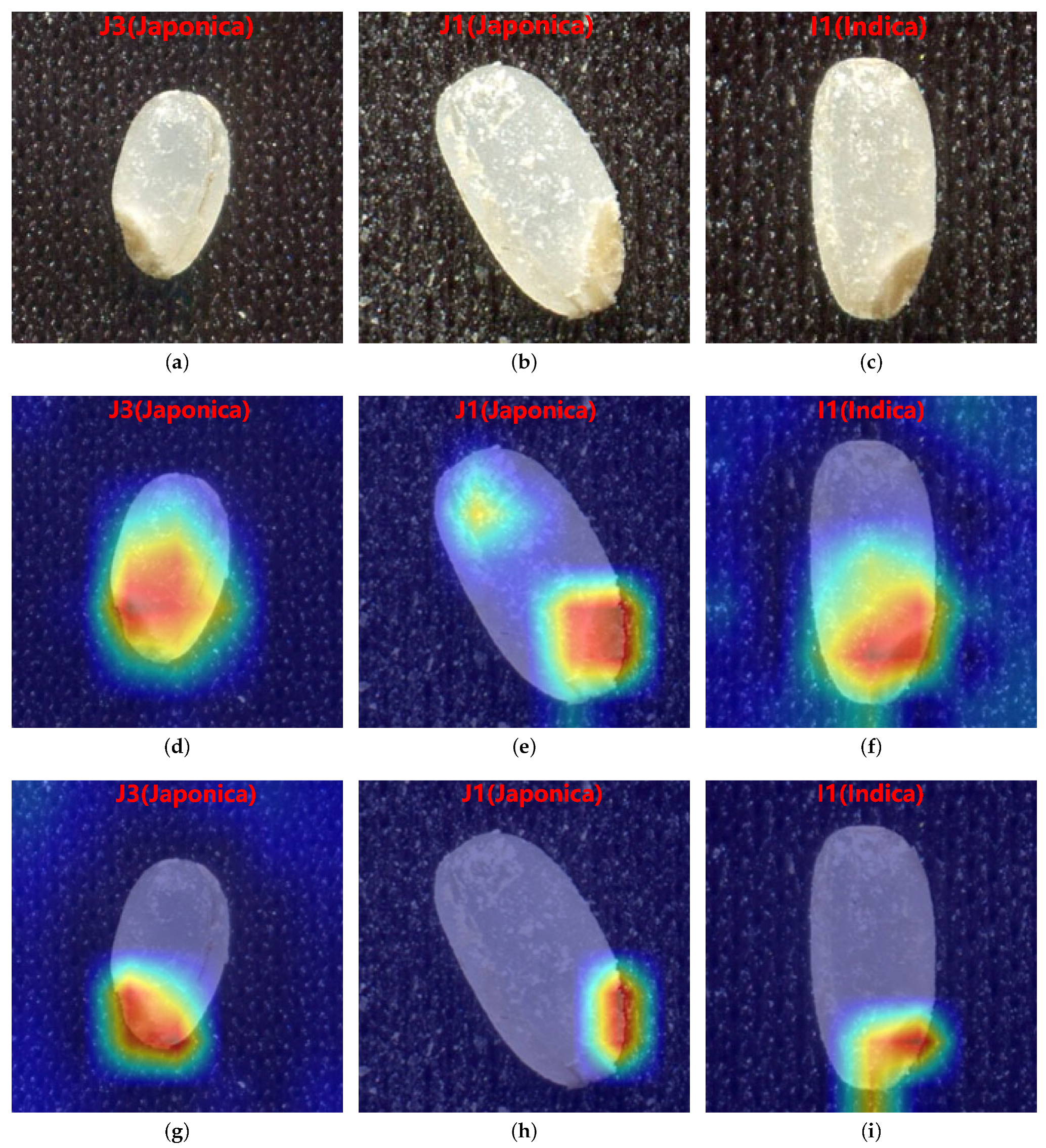
Figure 13.
The visualization comparison of three types of rice (J1, J3, I1) between original image (a–c), and attention heat map from EfficientNet–B3 (d–f), and EfficientNet–B3–DAN (g–i).
Figure 13.
The visualization comparison of three types of rice (J1, J3, I1) between original image (a–c), and attention heat map from EfficientNet–B3 (d–f), and EfficientNet–B3–DAN (g–i).


Table 1.
Types of rice.
| Label | Variety | Designation of Origin | Size | GPS Coordinates |
|---|---|---|---|---|
| J1 | Japonica | Suihua | Long | N: 46°38′14.28′′ E: 126°59′8.38′′ |
| J2 | Japonica | Wuping | Long | N: 25°05′43.26′′ E: 116°06′1.40′′ |
| J3 | Japonica | Yancheng | Short | N: 33°12′3.85′′ E: 120°30′3.67′′ |
| J4 | Japonica | Shuangyashan | Mid | N: 46°34′38.17′′ E: 131°24′6.41′′ |
| I1 | Indica | Wuping | Long | N: 25°05′43.26′′ E: 116°06′1.40′′ |
| I2 | Indica | Wuping | Long | N: 25°05′43.26′′ E: 116°06′1.40′′ |
Table 2.
Quantity of each type of rice.
| Dataset | 0–10% | 10–20% | 20–30% | 30–40% | 40–50% | 50–60% | 60–70% | 70–80% | 80–90% | 90–100% |
|---|---|---|---|---|---|---|---|---|---|---|
| Training dataset | 720 | 720 | 514 | 514 | 768 | 720 | 432 | 720 | 530 | 604 |
| Validation dataset | 240 | 240 | 170 | 170 | 256 | 240 | 143 | 240 | 176 | 200 |
| Test dataset | 240 | 240 | 170 | 170 | 256 | 240 | 143 | 240 | 176 | 200 |
Table 3.
Evaluation metrics of EfficientNet–B3–DAN.
| Class | TP 1 | TN 2 | FP 3 | FN 4 | Pre (%) 5 | Sen (%) 6 | Acc (%) 7 | F1-Score (%) | OA (%) 8 |
|---|---|---|---|---|---|---|---|---|---|
| 0–10% | 240 | 1834 | 1 | 0 | 100.00 | 100.00 | 99.95 | 100.00 | 94.17 |
| 10–20% | 240 | 1835 | 0 | 0 | 100.00 | 100.00 | 100.00 | 100.00 | |
| 20–30% | 167 | 1905 | 0 | 3 | 100.00 | 98.24 | 99.86 | 99.11 | |
| 30–40% | 170 | 1902 | 3 | 0 | 98.27 | 100.00 | 99.86 | 99.13 | |
| 40–50% | 203 | 1762 | 57 | 53 | 78.08 | 79.30 | 94.70 | 78.63 | |
| 50–60% | 179 | 1782 | 53 | 61 | 77.16 | 74.58 | 94.51 | 75.85 | |
| 60–70% | 142 | 1932 | 0 | 1 | 100.00 | 99.30 | 99.95 | 99.65 | |
| 70–80% | 237 | 1835 | 0 | 3 | 100.00 | 98.75 | 99.86 | 99.37 | |
| 80–90% | 176 | 1895 | 4 | 0 | 97.78 | 100.00 | 99.81 | 98.88 | |
| 90–100% | 200 | 1872 | 3 | 0 | 98.52 | 100.00 | 99.86 | 99.25 |
1 True Positive. 2 True Negative. 3 False Positive. 4 False Negative. 5 Precision(%). 6 Sensitivity(%). 7 Accuracy (%). 8 Overall accuracy (%).
Table 4.
Evaluation metrics of EfficientNet–B3–DAN.
| Model | AveragePre (%) | AverageSen (%) | AverageAcc (%) | AverageF1 (%) | OA (%) |
|---|---|---|---|---|---|
| AlexNet | 86.96 | 85.67 | 97.09 | 85.62 | 85.45 |
| VGG16 | 89.16 | 88.76 | 97.62 | 88.73 | 88.10 |
| ResNet50 | 90.18 | 88.74 | 97.54 | 88.11 | 87.71 |
| GoogleNet | 90.64 | 89.57 | 97.80 | 89.50 | 89.01 |
| MobileNet | 88.57 | 88.57 | 97.57 | 88.51 | 87.86 |
| EfficientNet–B3 | 91.75 | 91.64 | 98.10 | 91.35 | 90.51 |
| EfficientNet–B3–DAN | 94.94 | 95.02 | 98.84 | 94.97 | 94.17 |
Publisher’s Note: MDPI stays neutral with regard to jurisdictional claims in published maps and institutional affiliations. |
© 2022 by the authors. Licensee MDPI, Basel, Switzerland. This article is an open access article distributed under the terms and conditions of the Creative Commons Attribution (CC BY) license (https://creativecommons.org/licenses/by/4.0/).
Share and Cite
MDPI and ACS Style
Li, B.; Liu, B.; Li, S.; Liu, H. An Improved EfficientNet for Rice Germ Integrity Classification and Recognition. Agriculture 2022, 12, 863. https://0-doi-org.brum.beds.ac.uk/10.3390/agriculture12060863
AMA Style
Li B, Liu B, Li S, Liu H. An Improved EfficientNet for Rice Germ Integrity Classification and Recognition. Agriculture. 2022; 12(6):863. https://0-doi-org.brum.beds.ac.uk/10.3390/agriculture12060863
Chicago/Turabian StyleLi, Bing, Bin Liu, Shuofeng Li, and Haiming Liu. 2022. "An Improved EfficientNet for Rice Germ Integrity Classification and Recognition" Agriculture 12, no. 6: 863. https://0-doi-org.brum.beds.ac.uk/10.3390/agriculture12060863
Note that from the first issue of 2016, this journal uses article numbers instead of page numbers. See further details here.