

Tillage-Depth Verification Based on Machine Learning Algorithms
1
College of Agricultural Equipment Engineering, Henan University of Science and Technology, Luoyang 471003, China
2
Luoyang Xiyuan Vehicle and Power Inspection Institute Co., Ltd., Luoyang 471000, China
*
Author to whom correspondence should be addressed.
Agriculture 2023, 13(1), 130; https://0-doi-org.brum.beds.ac.uk/10.3390/agriculture13010130
Submission received: 29 November 2022
/
Revised: 24 December 2022
/
Accepted: 29 December 2022
/
Published: 4 January 2023
(This article belongs to the Special Issue Design and Application of Agricultural Equipment in Tillage System)
Abstract
:In an analysis of the penetration resistance and tillage depth of post-tillage soil, four surface-layer discrimination methods, specifically, three machine learning algorithms—Kmeans, DBSCAN, and GMM—and a curve-fitting method, were used to analyze data collected from the cultivated and uncultivated layers. Among them, the three machine learning algorithms found the boundary between the tilled and untilled layers by analyzing which data points belonged to which layer to determine the depth of the soil in the tilled layer. The curve-fitting method interpreted the intersection among data from the fitted curves of the ploughed layer and the un-ploughed layer as the tillage depth. The three machine learning algorithms were used to process a standard data set for model evaluation. DBSCAN’s discrimination accuracy of this data set reached 0.9890 and its F1 score reached 0.9934, which were superior to those of the other two algorithms. Under standard experimental conditions, the ability of DBSCAN clustering to determine the soil depth was the best among the four discrimination methods, and the discrimination accuracy reached 90.63% when the error was 15 mm. During field-test verification, the discriminative effect of DBSCAN clustering was still the best among the four methods. However, the soil blocks encountered in the field test affected the test data, resulting in large errors in the processing results. Therefore, the combined RANSCA robust regression and DBSCAN clustering algorithm, which can eliminate interference from soil blocks in the cultivated layer and can solve the problem of large depth errors caused by soil blocks in the field, was used to process the data. After testing, when the RANSCA and DBSCAN combined method was used to process all samples in the field and the error was less than 20mm, the accuracy rate reached 82.69%. This combined method improves the applicability of discrimination methods and provides a new method of determining soil depth.
1. Introduction
Soft soil is beneficial to the growth of crops, and fields that have been cultivated for many years will form a solid plough bottom, which hinders the penetration of precipitation into deep soil and is not conducive to the absorption of water by the crop roots. The depth of the tillage layer has a significant impact on agroecosystems and on crop yield and quality [1,2,3,4]. After the soil is loosened, the plow bottom can be broken, the plow-layer thickness can be increased, the soil structure can be improved, and the quality of cultivated land can be improved. In recent years, China has attached great importance to the quality of subsoiling operations, has encouraged farmers to prepare land for subsoiling operations, and has issued subsidies for subsoiling operations. At present, no unified standard has been accepted for automatically measuring the tillage depth in subsoiling operations. Manual sampling methods are often adopted but require manual cleaning of the ditch bottom, and human factors and soil conditions affect the measurement accuracy [5]. Moreover, manual determination of the tillage depth has a low efficiency, is labor-intensive, takes a long time, and provides a limited description of the tillage depth. Due to the importance of subsoiling land preparation and the need for supervision by the Ministry of Agriculture of China on, subsidies for subsoiling operations must be based on accurate information about the front-line operations of subsoiling machinery; thus, the demand for informatization identification and testing is quite high. Tillage depth is an important evaluation index of subsoiling quality, and accurate tillage-depth detection and control are very important. The determination of tillage depth by agricultural machinery equipment is mostly realized by one or more angle sensors, inclination sensors, attitude sensors, ultrasonic sensors, and infrared sensors.
The latest research on tillage-depth detection by domestic and foreign scholars can be divided into two types according to the detection method: non-contact and contact. Non-contact measurement methods are commonly used in the installation of ultrasonic sensors, particularly during the implementation of optical rangefinders on a replica wheel of the plow. Kim et al. [6] installed inclinometers and optical distance sensors on the left and right axes of linear potentiometers and used linear potentiometers and optical distance sensors to measure the depth of soil penetration. In addition, a single-axis inclinometer was used to measure the inclination angle during the tillage process, and the tillage depth was calculated based on the depth of the soil penetration and the pitch angle of the attached equipment. The conservation tillage popularized and applied in recent decades usually breaks up crop residues and mixes them with soil as nutrients for the next crop. However, neither ultrasonic sensors nor optical rangefinders can accurately distinguish crop residues from the ground. This affects the tillage-depth measurement, which greatly reduces the precision of the non-contact measurement method, and research on non-contact measurement methods has gradually decreased in recent years. In contrast, the contact measurement method has been increasingly studied, specifically, contact between the sensor and the actual soil surface. Mouazen et al. [7] connected a linear variable displacement sensor with a stroke length of 0–2 m to the frame of a metal wheel, with the height sensor located at the axle, and measured the swing-arm frame height. The distance between the soil surface and the frame changes, and an analytical–statistical hybrid model was built to calculate the change in the height of the frame. Xie et al. [8] developed a contact tillage-depth measurement method based on measuring the lift-arm inclination and the geometric relationship between the unit and the tractor. When measuring the tillage depth with this method, it is necessary to ensure that the plane of the plough body or the beam of the plough frame remains horizontal when the implemented frame reaches the maximum tillage depth. An irregular surface or a change in the slope affects the applicability and accuracy of the model. Afterwards, Jia Honglei et al. [9] designed an adaptive tillage-depth monitoring system that uses a photoelectric encoder to measure the angle between the adjustable swing arm. Based on different cases and corresponding mathematical models, they developed a LabVIEW program adapted to the measurement, which was slightly lacking in terms of real-time processing and visualization of the tillage depth. Overall, most non-contact technologies use ultrasonic rangefinders and optical rangefinders to indirectly measure the tillage depth, and most contact technologies use inclination sensors and angle-measuring instruments to indirectly measure the tillage depth. Although these methods provide an effective way to detect tillage depth and tillage quality online, each of these methods has certain problems. For example, when an inclination sensor is used to calculate the tillage depth, the sensor needs to be re-calibrated, which is inconvenient. Additionally, the detection accuracies of the angle-measuring instrument and the ultrasonic sensor are affected by surface debris.
To detect tillage depth, two methods are used: one is real-time monitoring of the tillage depth, and the other is identification detection. The testing equipment is usually placed on the machine for testing a rotary tillage operation in order to obtain real-time data of the operation. The experiments conducted by Kim et al. and Xie Bin et al., as described above, aimed to test the tillage depth in real time, as well as to verify and test the effect of their special testing equipment on rotary tillage. The goals of the abovementioned subsoiling preparation subsidies issued by the Ministry of Agriculture of China are to verify and test the subsoiling-preparation quality by measuring the tillage depth. However, some problems are found in the currently accepted methods of inspection, such as having inconsistent standards, producing large manual-measurement errors, and being labor-intensive. With the state strongly advocating for deep loose-land preparation, the Ministry of Agriculture and the Ministry of Finance attaches great importance to the subsoiling operations of the land, and subsidies for subsoiling operations must be issued based on accurate information about the front-line operations of subsoiling machinery. At present, the demand for information acceptance is quite strong. With the rapid development of autonomous navigation technology and information sensing technology in recent years, cultivated-land precision-monitoring technology has begun to become more refined and smarter. Additionally, verification and detection have become development trends in providing a quantitative basis for evaluating the quality of subsoiling operations by using sensors to determine tillage depth.
Machine learning algorithms often solve practical problems more efficiently due to the regularity information inherently found in data. In order to improve the automation and applicability of discriminating tillage depth, data on penetration resistance and tillage depth were analyzed. Finally, we decided to use four discrimination methods, specifically, three machine learning algorithms—Kmeans, DBSCAN, and GMM—as well as the curve fitting method, to analyze and compare the data from the cultivated layer and the uncultivated layer obtained in a laboratory experiment. Among them, the Kmeans algorithm clusters according to the distance similarity between the data points and the data points. The DBSCAN algorithm clusters according to the density of the data points, while the GMM algorithm clusters according to the assumption that the data points of each cluster conform to a Gaussian distribution of the corresponding cluster. The DBSCAN algorithm has the best effect in terms of determining tillage depth without any soil disturbance. In this paper, the Affinity propagation, Mean-shift, and OPTICS algorithms were also considered for use in distinguishing the surface layer. However, as Affinity propagation clustering [10] is carried out by sending messages between sample pairs until they converge, the number of clusters is determined according to the data provided, so distinguishing the binary classification problem between the cultivated layer and the uncultivated layer is ineffective. Mean-shift [11] is a density-based nonparametric clustering algorithm that needs to specify the candidate centroid and automatically sets the number of clusters. As the purpose of this experiment is to classify the number of specified clusters, this algorithm cannot be applied to distinguish the surface layer. The OPTICS algorithm [12] is a generalization of the DBSCAN algorithm. Clustering is performed according to density, but the number of clusters is automatically matched. Compared with DBSCAN, it is too sensitive and will divide the data into several clusters, meaning that it cannot solve the problem of plough layer discrimination. Furthermore, a field experiment was carried out to verify the ability of the methods to determine soil depth without any soil disturbance. The RANSCA robust regression algorithm is a kind of regression model that can be fitted into a regression model even if there are outliers or errors in the model. The use of a combination of this algorithm and the DBSCAN algorithm can solve the problem of soil disturbance discrimination and can accurately determine the tillage depth. The performance of the hybrid algorithm in field discrimination is not bad. The hybrid machine learning algorithm can greatly improve the production efficiency, reduce the labor intensity, and reduce the production cost. Thus, it provides a new method of determining topsoil depth.
2. Principle of Tillage-Depth Identification Based on Soil-Penetration Resistance
2.1. Test Instruments and Data Collection
In this paper, soil samples from Luoyang, Henan (34°39′47″ N, 112°26′4″ E), were used as the soil samples. First, the soil water content and density were measured by sampling in the field. The samples were measured with the sieving method and the hydrometer method, and obtained. The soil moisture content in the field ranged from 10% to 20%, and the soil density ranged from 1100 kg·m−3 to 1300 kg·m−3. Before conducting the soil-sample test to obtain the experimental data of the soil in the tilled and un-ploughed layers, the soil moisture content and density were divided into three levels for the orthogonal tests; the moisture content was taken as 10%, 15%, and 20%; and the density was taken as 1.1 × 10³ kg/m3, 1.2 × 10³ kg/m3, and 1.3 × 10³ kg/m3.
The equipment used to measure the soil moisture content and density range during field sampling in the indoor test includes a probe (material 65 Mn steel, length 530 mm, and maximum diameter of tip 14 mm), a universal testing machine (DNS02-1KW), and a barrel (inner diameter 124 mm and height 400 mm).
The specific operation steps in the test process are as follows:
- (1)
- Put about 5 kg of soil into the dryer for 48 h, and fully dry the soil.
- (2)
- Ensure that the height of the soil in the bucket is 300 mm. Calculate the required dry soil weight and water weight according to the inner diameter of the bucket, soil height, soil density, and moisture content.
- (3)
- Spray the soil until wet, and stir well to distribute the water evenly in the soil. Put the well-stirred soil into the bucket, turn the bucket upside down to decrease the distance between the soil surface and the top of the bucket to 100 mm, and ensure that the soil density reaches the required value.
- (4)
- Put the bucket filled with soil onto the frame of the universal testing machine, and install the probe. Open the analysis software, and adjust the probe height to ensure that the bottom of the probe is close to the soil surface. Adjust the penetration speed of the probe to 8 mm/s and the penetration depth to 300 mm, and run the software. For data acquisition, use the software installed on the computer. The software then exports the relationship between penetration resistance and penetration depth in an Excel file format. The simulated artificial soil-sample test diagram is shown in Figure 1.
- (5)
- The curve of penetration resistance and penetration depth can be obtained in real time during the test, and the test data can be saved after the test. The relationship between penetration resistance and penetration depth is shown in Figure 2 below.
- (6)
- Taking the moisture content of the tilled layer, the depth and density of the tilled layer, and the moisture content and density of the untilled layer as factors, the regression equation between the resistance of the stratification point and the maximum value of the untilled layer on the significant factors of tilled layer, moisture content, and density of untilled layer was established. If the surface layer depth is a significant factor, the surface-layer depth can be directly obtained from the maximum resistance value of the un-tilled layer. If the surface depth was not a significant factor, the resistance value of the stratified point was obtained from the regression equation and the surface depth was obtained from the experimental data. Thus, 32 groups of soil samples were prepared, each group was tested twice repeatedly, and a total of 64 sample data were obtained.
Figure 1.
Probe-penetration laboratory test.

Figure 2.
The relationship between penetration resistance and penetration depth.

2.2. The Principle of Machine Learning Algorithm in Discriminating the Depth of Cultivation
Soil-penetration resistance refers to the resistance of a conical or plunger-shaped penetration needle when penetrating into soil at a constant rate in an up–down direction due to the comprehensive effects of soil particle friction and extrusion. At the same sampling frequency, the soil in the cultivated layer is soft, so the penetration resistance of the cultivated layer increases with increasing penetration depth of the probe, and the collected data points are closely distributed. After years of cultivation in the field, a solid plough bottom layer is formed under the plough layer. When the probe enters the plough bottom layer, due to the soil firmness, the penetration resistance of the soil increases steeply, so the data points collected in the plough bottom layer are loosely distributed. Using a scatter plot and its corresponding mathematical analysis, the value of the cultivated depth of the measured point can be determined, and then, the method of determining the cultivated depth is verified as being feasible.
3. Basic Discriminant Methods and Their Comparisons
3.1. Kmeans Clustering Algorithm to Discriminate Cultivated Layer
The Kmeans clustering algorithm is one of the most commonly used methods in clustering. According to the similarity of the distance between points, the samples are separated into n groups with equal variance for clustering [13,14,15,16,17,18]. The Kmeans algorithm first randomly selects two data points as the centroids and from all the data points of the collected penetration resistance and penetration depth, with t as the number of iterations. The centroids chosen before iteration are marked as and , and these two centroids serve as the cluster centers before the tilled and un-tilled layers [13]. Based on the relationships between the data points, the objective of the optimization is defined before the clustering starts:
where c is the division of the data into two categories to distinguish between the cultivated layer and the uncultivated layer, c1 and c2, and M represents all data points, i.e., the total sample size.
The loop iteratively calculates the distance between each data point and the two cluster centers and , and the cluster center with the shortest distance when obtaining category is selected by dividing data point a into category at the t-th iteration.
where k is (j = 1,2) and the two clusters are obtained by processing all the data. The average distance of all sample points that are assigned to the same cluster is then calculated. The position of the average distance is used as the position of the new centroid of this iteration, that is, the new cluster centers and of this iteration, which must meet the following:
The iterative process is repeated until J converges, that is, the centroids of all clusters no longer change and the Kmeans discrimination of the tillage layer is completed.
Figure 3 shows the effect of data discrimination using Kmeans clustering. The position of the centroid is at “+” in the figure. When the centroid position remains unchanged, Kmeans iteratively processes all data and determines the soil depth of the plough layer.
All data points of the same cluster are marked with the same cluster number, and the boundary data of different clusters are found as the result of the discrimination of the soil depth of the tillage layer. After processing 64 groups of simulated surface-soil samples, the results show that four groups obtained absolute errors of less than 5 mm, twelve groups obtained absolute errors of less than 10 mm, twenty-six groups obtained absolute errors of less than 15 mm, and forty-seven groups obtained absolute errors of less than 20 mm.
3.2. DBSCAN Density Clustering Algorithm to Discriminate Tillage Layer
DBSCAN (density-based spatial clustering of applications with noise) density clustering treats clusters as low-density regions and high-density regions [19,20,21,22] and identifies a cluster class by classifying closely connected samples into one class [23,24]. The DBSCAN clustering algorithm is used to discriminate the soil depth of the cultivated layer. The radius eps (Eps-neighborhood of a point) of the cultivated layer data is set to 3.5, and the threshold min_samples is 4, that is, the data point of the cultivated layer is located in the radius eps of 3.5 and there are at least four samples in the field.
Since the penetration resistance of the un-ploughed layer increases due to the increased penetration resistance of the plow layer, the Euclidean distance between the collected sample points a(x1, y1) and b(x2, y2) increases, and the Euclidean distance d is as follows:
According to the data-distribution law of the cultivated layer and the uncultivated layer, a data point is randomly selected as the core point x1, and the Euclidean distance between other data points and the core point is used to determine whether other data points are densely connected. The basic algorithm principle model of DBSCAN is shown in Figure 4 below.
The core point x1 is randomly selected; a circle with eps as the radius is drawn; and the point in the center of the circle is the density direct access, that is, x2 is the density direct access of x1; x3, x4, and x1 are density accessible, x3 and x4 are density-connected, and all densities are connected. Cluster points are marked as data points of the same cluster. The density of the core point is compared with the threshold min_samples. If it is greater than or equal to the threshold min_samples, it is considered as a point in the same cluster. If it is less than the threshold min_samples, it is marked as a noise point and the noise point is marked as −1.
Due to the increase in penetration resistance, the data points collected in the un-ploughed layer cannot be densely connected with the data points of the cultivated layer and are marked as −1, which is an outlier. The first data point marked as an outlier, as discussed above, is the demarcation point between the tilled and uncultivated layers. The effect diagram for discriminating the DBSCAN’s soil tillage layer is shown in Figure 5 below.
The results obtained after clustering 64 groups of soil samples in the simulated tillage layer using the DBSCAN algorithm show that thirty-two groups had an absolute error of less than 5 mm, fifty-two groups had an absolute error of less than 10 mm, fifty-eight groups had an absolute error of less than 15 mm, and sixty groups had an absolute error of less than 20 mm.
3.3. Gaussian Mixture Model Clustering (GMM)
The Gaussian mixture model is usually referred to as GMM. It first assumes that there are k Gaussian distributions and then assesses the probability that each sample conforms to each distribution [25,26,27]. To determine the tillage depth, the samples are divided into two clusters: the tilled layer and the un-tilled layer, that is, k is 2. The sample data are then divided into the distribution cluster with the highest probability, maximum likelihood estimation is performed, the probability of conforming to the distribution of the cultivated layer and the uncultivated layer is calculated based on the new distribution, and the Gaussian distribution parameters are iteratively updated until the model uses the EM algorithm [28,29]. The convergence reaches the local optimal solution, the Gaussian function has good computational performance, and the probability density is often recorded as follows:
The Gaussian mixture distribution function required to define clustering is as follows:
Among them, represents the probability of each cluster, and the probability sum is 1, that is, . The data points are divided into corresponding clusters according to the probability . Finally, the conditional probability formula of whether a data point conforms to the cultivated layer or the uncultivated layer is as follows:
Each datum j then is found to conform to the corresponding cluster distribution probability for comparison, and the data points are divided into the corresponding clusters.
When the probability is calculated according to the formula, the probability density of a certain distribution in both the numerator and the denominator conforms to the Gaussian distribution, and the maximum likelihood method is used, that is, the maximum likelihood is performed according to the probability product of the corresponding distribution of the data:
Then, take the derivative of the above function, set the derivative to 0, and find the corresponding and :
Additionally, when calculating the corresponding Gaussian mixture coefficient , the Lagrange multiplier method needs to be added as a constraint, and the equation is obtained as follows:
The algorithm is as follows:
- 1
- Determine the two clusters for the cultivated layer and the un-ploughed layer, that is, k is 2;
- 2
- Initialize the Gaussian distribution parameters , , and of each cluster, and randomly assign them to construct the Gaussian mixture probability density;
- 3
- Traverse all sample data, and calculate the conditional probability that each sample conforms to each distribution, that is ;
- 4
- Then, use the calculated to calculate new values for , , and ; update the distribution model with the new parameters; and obtain a new probability density;
- 5
- Use the new distribution model to calculate the conditional probability of each sample, repeat steps (2)–(4), continuously update the model distribution parameters until the model converges, and then stop the iteration;
- 6
- Obtain the conditional probability of each sample based on the new model parameters, and then, obtain the maximum value of , as the clustering result of these data.
The schematic diagram of the GMM clustering density estimation is shown in Figure 6. The darker the color is, the larger the density estimation is, and the lighter the color is, the smaller the density estimation is. The GMM discriminant effect is shown in Figure 7.
The clustering result of the GMM algorithm marks the cultivated layer as a cluster 1, which is the yellow data point in Figure 7; the un-ploughed layer data are a cluster marked as 0, which is the black and purple data point in Figure 7. The results obtained after processing 64 groups of soil samples in the simulated tillage layer show that the number of samples with an absolute error less than 5 mm is 31, the number of samples with an absolute error less than 10 mm is 48, the number of samples with an error less than 15 mm is 52, and the number of samples with an error less than 20 mm is 59 groups.
3.4. Data Fitting to Determine Tillage Depth
After the soil is compacted, physical properties such as bulk density, porosity, and temperature of the soil change compared with the soil before compaction, and the root penetration resistance also increases. The working principle of the rotary tiller is that the blade of the rotary tiller rotates at a certain speed and moves forward in random groups to make up the milling process: soil cutting, crushing, and throwing back. Therefore, physical properties such as bulk density, porosity, and temperature of the soil in the plough layer that have been rotary tilled tend to be the same. Since the soil in the plough bottom layer has not been ploughed for many years, it forms a solid plough bottom layer under the plough layer. Thus, a plow bottom layer 40–50 cm below the plough layer tends to maintain the same physical properties.
According to Yan Ben [29], depth and penetration resistance share a quadratic polynomial relationship, and the soil-sample data were collected at a uniform speed. Therefore, data fitting was performed according to the theory that depth and penetration resistance share a quadratic polynomial relationship.
A portion of the data for the tilled layer and a portion of the data for the uncultivated layer were intercepted, and quadratic curves were fitted to the depth and penetration resistance. The penetration resistance of the soil in the plough layer increases with the penetration depth, so it is inferred that this point is the boundary where the plough layer meets the un-ploughed layer. The original data before data fitting are shown in Figure 8, and the fitted quadratic curve is shown in Figure 9:
Sixty-four groups of soil samples were processed by fitting quadratic curves to find the intersection points. The number of soil samples with an error of less than 5 mm was 24, the number of samples with errors less than 10 mm was 47, the number of samples with errors less than 15 mm was 55, and the number of samples with errors less than 20 mm was 60.
3.5. Comparison of Evaluation Results of Three Kinds of Machine Learning
This paper mainly deals with the problem of binary classification and takes the above curve data as a standard data set of the simulated soil samples. The accuracy rate, accuracy rate, recall rate, and F1 function of the clustering results from the three machine learning algorithms were evaluated [30]:
TP (True Positive) = True positive: a positive sample is correctly predicted to be positive
FP (False Positive) = False positive: a negative sample is incorrectly predicted to be positive
FN (False Negative) = False negative: a positive sample is incorrectly predicted to be negative
TN (True Negative) = True negative: a negative sample is correctly predicted to be negative
Accuracy refers to the percentage of cases in which predictions are correct:
Precision refers to the percentage of positive cases in which the prediction is correct:
Recall refers to the percentage of cases that are actually positive and are predicted correctly:
F1 score takes the precision rate and recall rate into consideration. When both are high, the values are balanced:
The above three machine learning algorithms are evaluated against the results of the standard data set, and the results are shown in Table 1 below.
It can be seen from the above table that the DBSCAN algorithm has the best performance for the classification of this standard data set, with an accuracy of 0.9890 and an F1 score of 0.9934, which are superior to those of the other two algorithms.
3.6. Comparison of the Effects of Several Methods in Discriminating the Plough Layer
The 64 groups of simulated soil samples are summarized in Table 2 according to the statistical data on the clustering effect.
According to the above table, the best clustering effect is clearly DBSCAN. When the error is within 15 mm, the accuracy of the DBSCAN clustering algorithm in discriminating the tillage layer is 90.63%; when the error is less than 20 mm, the accuracy rate reaches 93.75%. In terms of the discriminant effect, DBSCAN clustering has the best discriminative effect, data fitting has the second-best discriminant effect, GMM clustering has the third best discriminant effect, and Kmeans clustering has the worst discriminant effect.
4. Field-Test-Specific Situation and Hybrid Algorithm
4.1. Field-Data Collection
The equipment used in the field experiment was a multi-point probe-type tillage section detection vehicle designed by our team (Figure 10). The inspection vehicle has six probes, with a side-by-side spacing of 20 cm. Each probe has a force sensor and a displacement sensor to collect data at the same time. The data from the six probes were collected and transmitted to the computer for subsequent data analysis. After collecting the data for a section, the inspection vehicle moves forward by 20 cm. The location of the field experiment was Mengjin County, Luoyang City (34.819° N, 112.3901° E).
Because the firmness of the soil in the field is much larger than that of the soil samples in the laboratory, it was found in the actual field experiment that the data collected by the probe have a disturbance area; the disturbance area is found in the ploughed layer and is close to the plow bottom. When the probe enters the disturbance area of the soil, the penetration resistance increases significantly before it even touches the plow bottom. In the simulation of soil penetration resistance in the field, our team found that the shear modulus of the soil at the bottom of the plough is significantly larger than that of the tilled layer, such that the soil firmness is greater than that of the tilled layer. When the disturbance area is close to the bottom of the plow, the probe continues to penetrate, and the depth of the disturbance area gradually decreases. However, the existence of a disturbance area causes the machine learning algorithm to make a larger error when discriminating the soil depth of the ploughed layer. Our team simulated a large amount of data on the soil ploughed layer in the field to determine that the disturbed area is located 20–30 mm above the ploughed and un-ploughed layers. In order to determine the applicability of the algorithm, an average value of 25 mm was selected as the systematic error for discriminating the cultivated layer in the field test.
4.2. Discrimination Effect of the Four Methods for Discriminating the Plough Layer in the Field Test
According to the agronomic requirements, the rotary tillage operation allows for the existence of clods within a certain range. When collecting data in the field experiment, since the maximum diameter of the probe is 14 mm, it is inevitable that the probe collects data vertically in a downwards direction and hits the clods. Therefore, the field experiment collects two types of data: one is data that do not encounter the clods, and the other is data that encounter the clods. The data collected without encountering clods and the Kmeans clustering, DBSCAN clustering, and GMM clustering discrimination effect are shown in Figure 11.
Among the methods, Kmeans clustering sets the parameter k as 2 to obtain two clusters, and the data point output of the first cluster is used as the boundary at which Kmeans clustering discriminates the cultivated layer. DBSCAN sets the parameter eps to 7 and min_samples to 5, that is, when the radius is 7, there are 5 sample points, and the data point is output when the first outlier is used is the boundary at which DBSCAN clustering discriminates the cultivated layer. Parameter k from GMM clustering is set to 2, and the data point output from the first different cluster is used as the boundart at which GMM clustering discriminates the cultivated layer. Additionally, MATLAB data fitting takes the intersection as the cut-off point of the tillage layer. A total of 52 groups of field samples were collected, and 41 groups of field samples were obtained in the case of no soil blocks. The clustering effect statistics for the cultivated layer data are shown in Table 3 below.
It can be seen from the above table that when the error is less than 20 mm, the accuracy rate of DBSCAN in discriminating the cultivated layer is 90.24%. The effect of DBCSAN clustering when discriminating the cultivated layer is still the best in the field test; followed by data fitting; and then, GMM clustering when discriminating the cultivated layer, and Kmeans still has the worst results.
4.3. RANSCA Robust Regression Algorithm to Deal with the Error of the Soil Block
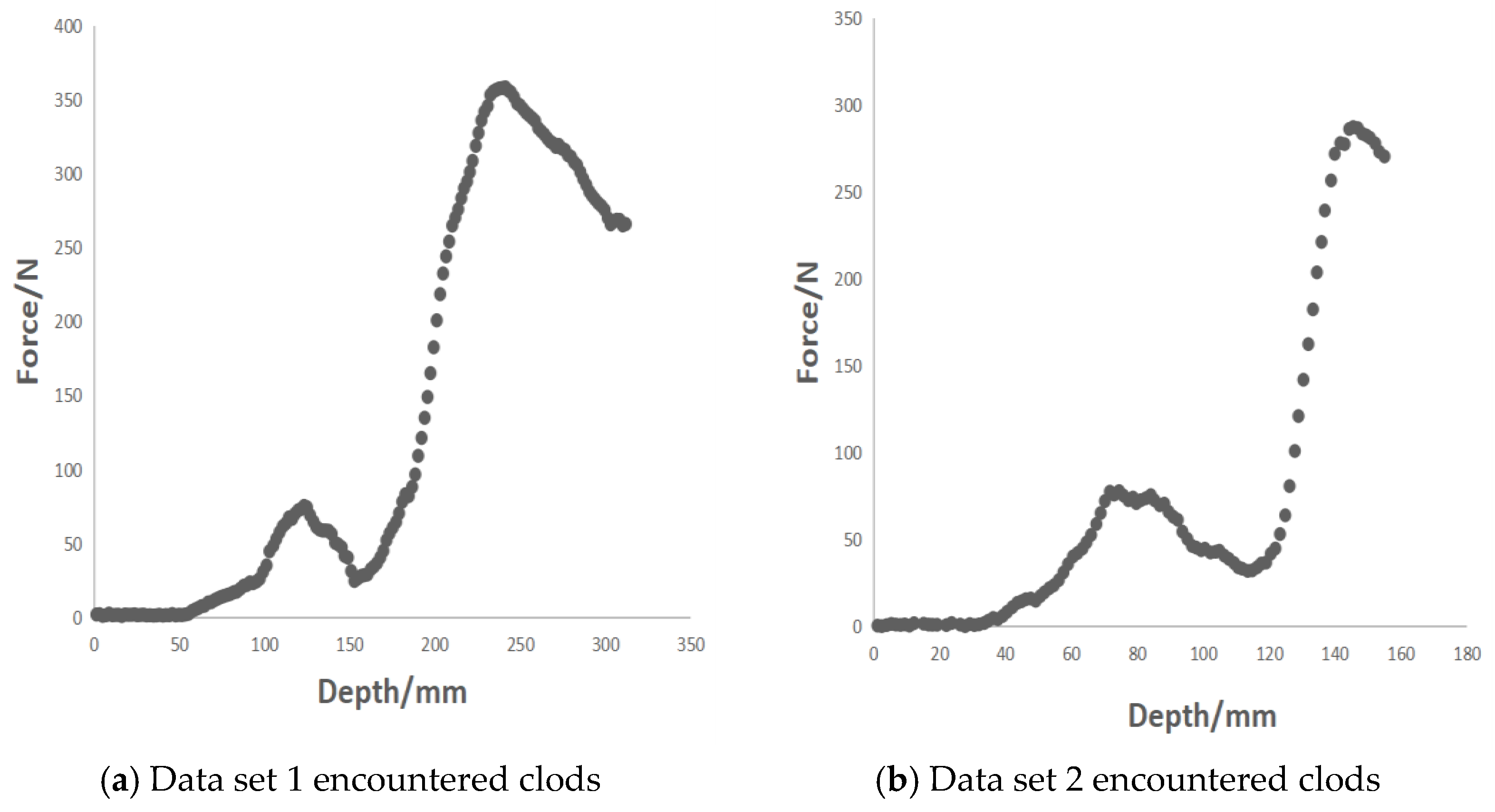
When collecting the data, 11 groups of sample data were found to have encountered soil blocks. The sample data collected for the soil blocks are shown in Figure 12.
When encountering clods, several clustering methods determined the collected soil block data as the boundary point of the cultivated layer, resulting in a particularly large discrimination error. Thus, a new method is needed to solve the problem of encountering clods. In this paper, a hybrid RANSCA (random sample consensus) robust regression algorithm and DBSCAN clustering algorithm is proposed to discriminate the tillage layer.
The RANSCA algorithm fits a regression model in the presence of bad data (i.e., there are outliers or errors in the model) [31]. RANSAC is a non-deterministic algorithm that produces a reasonable result with a certain probability [32]. The basic assumption of the RANSCA algorithm is that the sample contains correct data (data that can be described by the model), called “inliers”. Data that that cannot fit the mathematical model are called “outliers”, i.e., the data set contains noise. The basic assumptions of the RANSCA algorithm are as follows:
- (1)
- The data consists of correct data, namely “inliers”, and the distribution of “inliers” can be used to calculate a model;
- (2)
- “Outliers” are parameters that cannot be adapted to the model;
- (3)
- Other data are noise.
Through an analysis of the curve diagram of penetration resistance and penetration depth, it can be found that, when no soil clods are encountered, the model calculated by fitting all the data of the surface layer is identified as the “local point”. When dirt clods are encountered, the data points collected do not fit the calculated model and are identified as “external points”. Data points that are determined to be “intra-office” after RANSCA robust regression are marked as true, and data points that are determined to be external are marked as false. It can be seen from the above that the data points before those considered true by the RANSAC robust regression algorithm are all points collected in the cultivated layer. RANSCA fits the regression model for the cultivated layer data and allows for noise. Even under discrimination by DBSCAN density clustering, the soil clod data encountered cannot be divided into a cluster with other cultivated layer data [33], but because the data are identified as a cultivated layer by the RANSCA algorithm, the data encountering soil clods are not regarded as the result of DBSCAN discriminating a plough layer. The RANSCA algorithm solves the problem of the inability of the DBSCAN algorithm to cluster soil clod data and other cultivated layer data.
4.4. The Hybrid RANSCA and DBSCAN Algorithm Identifies the Soil Topsoil Layer
The cultivable layer is simultaneously identified by each part of the hybrid algorithm. That is, the first data point considered an outlier by DBSCAN after RANSCA discriminates the last true data point is used as the boundary between the cultivable layer and the uncultivable layer. The steps in RANSCA robust regression and DBSCAN clustering hybrid algorithm are as follows:
- (1)
- First, the data from the cultivated layer are used as the data set for RANSAC training, and a set of random subsets in the data set are selected as “inliers” to train the model. The unknown parameters of the model are calculated from hypothetical “inliers”.
- (2)
- The obtained model is then used to test other data. If other data are also applicable to this model, they are considered “inliers”. If enough points are considered “inliers”, the model is proven to be reasonable enough.
- (3)
- The model is then re-estimated with all of the “inliers”. If the generated model has too few “inliers”, it is discared and replaced with a better model until the final model is determined.
- (4)
- After the model is determined, data points that encounter a soil block and are not suitable for the model are considered “outliers” and marked as false, and all data before the last data point considered “inliers” are regarded as the cultivated layer data.
- (5)
- All data are clustered by DBSCAN clustering, and the first “outliers” after all of the data points for the cultivated layer are used as the basis for the discrimination of the cultivated layer.
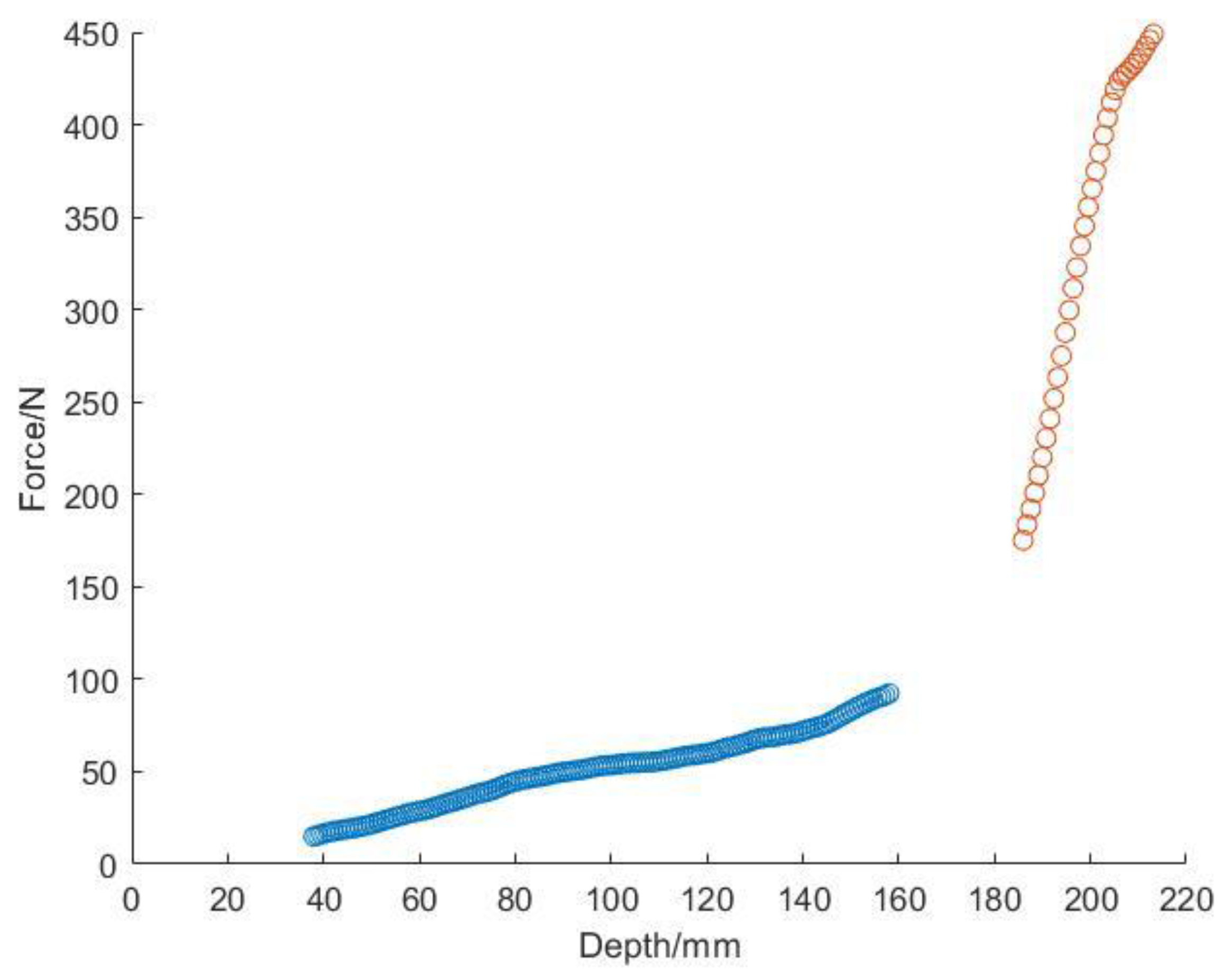
The discriminant flow chart and a diagram of the effect are shown in Figure 13. The rendering diagram of the data set for discriminating the encounter of soil clods is shown in Figure 14.
The hybrid algorithm can discriminate the tillage layer, and the discriminant effect basically is ineffective when no soil block is encountered. The discriminant effect diagram is as follows. The discriminant effect diagram is shown in Figure 15 below.
The 41 groups of field samples that did not encounter soil blocks were processed with DBSCAN and the combined RANSCA and DBSCAN algorithm, as well as the combined RANSCA and DBSCAN clustering to process all of the field samples of the 51 groups. The results are shown in Table 4 below.
By comparing the results of DBSCAN clustering and the hybrid algorithm when dealing with unencountered soil blocks, it can be found that the hybrid algorithm has almost no influence on the discrimination of the surface layer when no soil blocks are encountered.
Moreover, the hybrid algorithm can solve the problem of a soil block encountered by the probe in the field, avoids interference from the soil block in the surface discrimination, and makes the discrimination method more applicable. When the error is less than 20 mm, the accuracy of the RANSCA and DBSCAN hybrid algorithm is 82.69%, and the performance of the hybrid algorithm in the field experiment is fair.
5. Conclusions
In this paper, three machine learning algorithms were used to process a standard data set for model evaluation in an indoor manual soil-sample test. Among them, the discrimination accuracy of DBSCAN for the data set reached 0.9890 and the F1 score reached 0.9934, which was better than those of the other two algorithms. At the same time, 64 groups of simulated soil-sample data were processed with DBSCAN and the discrimination accuracy was 90.63% when the error was less than 15 mm and 93.75% when the error was less than 20 mm, which verified that DBSCAN had a better discrimination effect than Kmeans clustering, GMM clustering, and data fitting.
In the field experiment, since the maximum diameter of the tip of the probe is 14 mm, it is almost impossible to rotate until all of the soil in the tilled layer becomes loose during mechanical operation. Whether rotating the till or the deep till, there can be soil clods within the range allowed by agronomy. That is to say, it is inevitable that there will be soil clods with a diameter of more than 14mm in the soil during a rotary tillage operation. When the probe goes straight down to assess penetration resistance, it inevitably hits small clods that are not completely broken. Therefore, data processing in the field can be divided into two conditions: no clods encountered and clods encountered. When no soil clods were encountered and the error was less than 20 mm, the accuracy of DBSCAN in identifying a plough layer was 90.24%. When comparing the four discriminant methods, DBSCAN still had the best discriminant effect on the soil layer. However, the soil clods encountered in the field experiment will affect the test data and cause significant errors in the processing results. Therefore, the combined RANSCA robust regression and DBSCAN clustering algorithm was used in this paper to process the collected data. When the mixed algorithm processed the data without encountering soil clods, the accuracy was not affected. When the error was less than 20 mm, the accuracy of the mixed algorithm reached 92.68%. At the same time, the hybrid algorithm eliminates the disturbance due to soil clods and determines the ploughing depth, which solves the problem of the large ploughing depth error caused by soil clods in the field. It has been verified that the combined RANSCA and DBSCAN method of discriminating the soil depth of topsoil in the field with an error of less than 20 mm can reach an accuracy of 82.69%. The error in distinguishing soil depth caused by soil clods in the field is thus solved. The combined RANSCA robust regression and DBSCAN clustering algorithm improved the applicability of the discrimination method and provided a new method for verifying and discriminating topsoil depth. It can be widely used to evaluate the quality of subsoiling operations and in assessing whether subsoiling land preparation subsidies should be issued by the Ministry of Agriculture of China. The tillage depth can be accurately determined by measuring only the penetration resistance and depth, making the information acceptance tests refined and smart.
Author Contributions
Conceptualization, J.P.; methodology, X.Z. and X.L.; software, X.Z.; formal analysis, J.L., X.D. and J.H.; writing—original draft preparation, J.P. and X.Z. All authors have read and agreed to the published version of the manuscript.
Funding
This work was supported by the National Key R&D Program of China (Grant No. 2017YFD0700300).
Institutional Review Board Statement
Not applicable.
Informed Consent Statement
Informed consent was obtained from all subjects involved in the study.
Data Availability Statement
All data sets in this article were collected by the team.
Conflicts of Interest
The authors declare no conflict of interest.
References
- Jin, C.; Pang, D.; Min, J.I.N.; Luo, Y.L.; Li, H.Y.; Yong, L.I.; Wang, Z.L. Improved soil characteristics in the deeper plough layer can increase grain yield of winter wheat. J. Integr. Agric. 2020, 19, 1215–1226. [Google Scholar] [CrossRef]
- Arvidsson, J.; Håkansson, I. A model for estimating crop yield losses caused by soil compaction. Soil Tillage Res. 1991, 20, 319–332. [Google Scholar] [CrossRef]
- Olesen, J.E.; Munkholm, L.J. Subsoil loosening in a crop rotation for organic farming eliminated plough pan with mixed effects on crop yield. Soil Tillage Res. 2007, 94, 376–385. [Google Scholar] [CrossRef]
- Yamazaki, H.; Yoshida, T. Various scarification treatments produce different regeneration potentials for trees and forbs through changing soil properties. J. For. Res. 2020, 25, 41–50. [Google Scholar] [CrossRef]
- Zikeli, S.; Gruber, S. Reduced tillage and no-till in organic farming systems, Germany—Status quo, potentials and challenges. Agriculture 2017, 7, 35. [Google Scholar] [CrossRef] [Green Version]
- Kim, Y.S.; Kim, T.J.; Kim, Y.J.; Lee, S.D.; Park, S.U.; Kim, W.S. Development of a real-time tillage depth measurement system for agricultural tractors: Application to the effect analysis of tillage depth on draft force during plow tillage. Sensors 2020, 20, 912. [Google Scholar] [CrossRef] [Green Version]
- Mouazen, A.M.; Anthonis, J.; Saeys, W.; Ramon, H. An automatic depth control system for online measurement of spatial variation in soil compaction, Part 1: Sensor design for measurement of frame height variation from soil surface. Biosyst. Eng. 2004, 89, 139–150. [Google Scholar] [CrossRef]
- Xie, B.; Li, H.; Zhu, Z.X. Automatic measurement method of tillage depth of tractor suspension unit based on inclination sensor. Trans. Chin. Soc. Agric. Eng. 2013, 29, 15–21. [Google Scholar] [CrossRef]
- Jia, H.; Guo, M.; Yu, H.; Li, Y.; Feng, X.; Zhao, J.; Qi, J. An adaptable tillage depth monitoring system for tillage machine. Biosyst. Eng. 2016, 151, 187–199. [Google Scholar] [CrossRef]
- Bodenhofer, U.; Kothmeier, A.; Hochreiter, S. APCluster: An R package for affinity propagation clustering. Bioinformatics 2011, 27, 2463–2464. [Google Scholar] [CrossRef] [Green Version]
- Peng, K.; Leung, V.C.M.; Huang, Q. Clustering approach based on mini batch kmeans for intrusion detection system over big data. IEEE Access 2018, 6, 11897–11906. [Google Scholar] [CrossRef]
- Ankerst, M.; Breunig, M.M.; Kriegel, H.P.; Sander, J. OPTICS: Ordering points to identify the clustering structure. ACM Sigmod Rec. 1999, 28, 49–60. [Google Scholar] [CrossRef]
- Ahmed, M.; Seraj, R.; Islam, S.M.S. The k-means algorithm: A comprehensive survey and performance evaluation. Electronics 2020, 9, 1295. [Google Scholar] [CrossRef]
- Abubaker, M.; Ashour, W.M. Efficient data clustering algorithms: Improvements over Kmeans. Int. J. Intell. Syst. Appl. 2013, 5, 37–49. [Google Scholar] [CrossRef] [Green Version]
- Sinaga, K.P.; Yang, M.S. Unsupervised K-means clustering algorithm. IEEE Access 2020, 8, 80716–80727. [Google Scholar] [CrossRef]
- Likas, A.; Vlassis, N.; Verbeek, J.J. The global k-means clustering algorithm. Pattern Recognit. 2003, 36, 451–461. [Google Scholar] [CrossRef] [Green Version]
- Adnan, R.M.; Khosravinia, P.; Karimi, B.; Kisi, O. Prediction of hydraulics performance in drain envelopes using Kmeans based multivariate adaptive regression spline. Appl. Soft Comput. 2021, 100, 107008. [Google Scholar] [CrossRef]
- Zahra, S.; Ghazanfar, M.A.; Khalid, A.; Azam, M.A.; Naeem, U.; Prugel-Bennett, A. Novel centroid selection approaches for KMeans-clustering based recommender systems. Inf. Sci. 2015, 320, 156–189. [Google Scholar] [CrossRef]
- Hahsler, M.; Piekenbrock, M.; Doran, D. dbscan: Fast density-based clustering with R. J. Stat. Softw. 2019, 91, 1–30. [Google Scholar] [CrossRef] [Green Version]
- Schubert, E.; Sander, J.; Ester, M. DBSCAN revisited, revisited: Why and how you should (still) use DBSCAN. ACM Trans. Database Syst. (TODS) 2017, 42, 1–21. [Google Scholar] [CrossRef]
- Khan, K.; Rehman, S.U.; Aziz, K.; Fong, S.; Sarasvady, S. DBSCAN: Past, present and future. In Proceedings of the Fifth International Conference on the Applications of Digital Information and Web Technologies (ICADIWT 2014), Chennai, India, 17–19 February 2014; IEEE: Toulouse, France, 2014; pp. 232–238. [Google Scholar] [CrossRef]
- Weng, S.; Gou, J.; Fan, Z. $ h $-DBSCAN: A simple fast DBSCAN algorithm for big data. Asian Conf. Mach. Learn. PMLR 2021, 157, 81–96. [Google Scholar]
- Chen, Y.; Zhou, L.; Bouguila, N.; Wang, C.; Chen, Y.; Du, J. BLOCK-DBSCAN: Fast clustering for large scale data. Pattern Recognit. 2021, 109, 107624. [Google Scholar] [CrossRef]
- Luchi, D.; Rodrigues, A.L.; Varejão, F.M. Sampling approaches for applying DBSCAN to large datasets. Pattern Recognit. Lett. 2019, 117, 90–96. [Google Scholar] [CrossRef]
- Windmeijer, F. A finite sample correction for the variance of linear efficient two-step GMM estimators. J. Econom. 2005, 126, 25–51. [Google Scholar] [CrossRef]
- Roodman, D. How to do xtabond2: An introduction to difference and system GMM in Stata. Stata J. 2009, 9, 86–136. [Google Scholar] [CrossRef] [Green Version]
- Campbell, W.M.; Sturim, D.E.; Reynolds, D.A. Support vector machines using GMM supervectors for speaker verification. IEEE Signal Process. Lett. 2006, 13, 308–311. [Google Scholar] [CrossRef]
- McLachlan, G.J.; Krishnan, T. The EM Algorithm and Extensions; John Wiley & Sons: Hoboken, NJ, USA, 2007. [Google Scholar]
- Yan, B. Research and Measurement Device Design of the Penetration Resistance of Granular Materials; Northeast Agricultural University: Harbin, China, 2018. [Google Scholar]
- Nabipour, M.; Nayyeri, P.; Jabani, H.; Shahab, S.; Mosavi, A. Predicting stock market trends using machine learning and deep learning algorithms via continuous and binary data; a comparative analysis. IEEE Access 2020, 8, 150199–150212. [Google Scholar] [CrossRef]
- Guo, Q.; Hu, X. Power line icing monitoring method using binocular stereo vision. In Proceedings of the 2017 12th IEEE Conference on Industrial Electronics and Applications (ICIEA), Siem Reap, Cambodia, 18–20 June 2017; IEEE: Toulouse, France, 2017; pp. 1905–1908. [Google Scholar] [CrossRef]
- Ruiz, L.A.; Fdez-Sarría, A.; Recio, J.A. Texture feature extraction for classification of remote sensing data using wavelet decomposition: A comparative study. In Proceedings of the 20th ISPRS Congress, Istanbul, Turkey, 12–23 July 2004; Volume 35, pp. 1109–1114. [Google Scholar]
- Kumar, K.M.; Reddy, A.R.M. A fast DBSCAN clustering algorithm by accelerating neighbor searching using Groups method. Pattern Recognit. 2016, 58, 39–48. [Google Scholar] [CrossRef]
Figure 3.
Kmeans processing data-discrimination effect diagram.

Figure 4.
Principle model diagram of the basic algorithm of DBSCAN.

Figure 5.
Discrimination effect diagram of a soil tillage layer by DBSCAN.

Figure 6.
Schematic diagram of the density estimation of the GMM.

Figure 7.
GMM clustering discrimination effect diagram.

Figure 8.
Schematic diagram of the original data points in the cultivated layer and the un-ploughed layer.
Figure 8.
Schematic diagram of the original data points in the cultivated layer and the un-ploughed layer.

Figure 9.
Schematic diagram of MATLAB fitting curve.

Figure 10.
Image of multi-point probe-type tillage section inspection vehicle used in the field test.
Figure 10.
Image of multi-point probe-type tillage section inspection vehicle used in the field test.

Figure 11.
Discrimination-effect of the clustering methods in the field test.

Figure 12.
The original data collected when encountering clods in the field.

Figure 13.
Data flow diagram of RANSCA and DBSCAN hybrid algorithm processing.

Figure 14.
Schematic diagram of the RANSCA and DBSCAN hybrid algorithm processing the data encountered in the clod. (a) The hybrid algorithm processes the encountered clod data set 1. (b) The hybrid algorithm processes the encountered clod data set 2.
Figure 14.
Schematic diagram of the RANSCA and DBSCAN hybrid algorithm processing the data encountered in the clod. (a) The hybrid algorithm processes the encountered clod data set 1. (b) The hybrid algorithm processes the encountered clod data set 2.

Figure 15.
Schematic diagram of the RANSCA and DBSCAN hybrid algorithm processing data that did not encounter clods.
Figure 15.
Schematic diagram of the RANSCA and DBSCAN hybrid algorithm processing data that did not encounter clods.


Table 1.
Results from the comparison of the three machine learning algorithms.
| Accuracy | Precision | Recall | F1 Score | |
|---|---|---|---|---|
| DBSCAN | 0.9890 | 1 | 0.9868 | 0.9934 |
| Kmeans | 0.9706 | 0.966 | 1 | 0.9827 |
| GMM | 0.9080 | 1 | 0.889 | 0.9412 |
Table 2.
Statistical data on the clustering effect of the simulated soil samples.
| Kmeans Clustering | DBSCAN Clustering | GMM Clustering | Data Fitting | |||||
|---|---|---|---|---|---|---|---|---|
| Sample Size | Accuracy | Sample Size | Accuracy | Sample Size | Accuracy | Sample Size | Accuracy | |
| Error < 5 mm | 4 | 6.25% | 32 | 50% | 31 | 48.44% | 24 | 37.5% |
| Error < 10 mm | 12 | 18.75% | 52 | 81.25% | 48 | 75% | 47 | 73.44% |
| Error < 15 mm | 26 | 40.63% | 58 | 90.63% | 52 | 81.25% | 55 | 85.94% |
| Error < 20 mm | 47 | 73.44% | 60 | 93.75% | 59 | 92.19% | 60 | 93.75% |
Table 3.
Statistical data on clustering effect of field soil samples.
| Kmeans Clustering | DBSCAN Clustering | GMM Clustering | Data Fitting | |||||
|---|---|---|---|---|---|---|---|---|
| Sample Size | Accuracy | Sample Size | Accuracy | Sample Size | Accuracy | Sample Size | Accuracy | |
| Error < 5 mm | 5 | 12.2% | 14 | 34.15% | 10 | 24.4% | 9 | 21.95% |
| Error < 10 mm | 7 | 17.07% | 30 | 73.17% | 21 | 51.22% | 20 | 48.78% |
| Error < 15 mm | 11 | 26.83% | 36 | 87.8% | 26 | 63.41% | 26 | 63.41% |
| Error < 20 mm | 25 | 60.98% | 37 | 90.24% | 32 | 78.05% | 31 | 75.61% |
Table 4.
Comparison of DBSCAN clustering and hybrid clustering effects.
| DBSCAN Clustering Results | RANSCA and DBSCAN Did Not Encounter Clod Results | RANSCA and DBSCAN Encountered Clod Results | ||||
|---|---|---|---|---|---|---|
| Sample Size | Accuracy | Sample Size | Accuracy | Sample Size | Accuracy | |
| Error < 5 mm | 14 | 34.15% | 14 | 34.15% | 16 | 30.77% |
| Error < 10 mm | 30 | 73.17% | 28 | 68.29% | 32 | 53.85% |
| Error < 15 mm | 36 | 87.8% | 32 | 78.05% | 38 | 69.23% |
| Error < 20 mm | 37 | 90.24% | 38 | 92.68% | 45 | 82.69% |
Disclaimer/Publisher’s Note: The statements, opinions and data contained in all publications are solely those of the individual author(s) and contributor(s) and not of MDPI and/or the editor(s). MDPI and/or the editor(s) disclaim responsibility for any injury to people or property resulting from any ideas, methods, instructions or products referred to in the content. |
© 2023 by the authors. Licensee MDPI, Basel, Switzerland. This article is an open access article distributed under the terms and conditions of the Creative Commons Attribution (CC BY) license (https://creativecommons.org/licenses/by/4.0/).
Share and Cite
MDPI and ACS Style
Pang, J.; Zhang, X.; Lin, X.; Liu, J.; Du, X.; Han, J. Tillage-Depth Verification Based on Machine Learning Algorithms. Agriculture 2023, 13, 130. https://0-doi-org.brum.beds.ac.uk/10.3390/agriculture13010130
AMA Style
Pang J, Zhang X, Lin X, Liu J, Du X, Han J. Tillage-Depth Verification Based on Machine Learning Algorithms. Agriculture. 2023; 13(1):130. https://0-doi-org.brum.beds.ac.uk/10.3390/agriculture13010130
Chicago/Turabian StylePang, Jing, Xuwen Zhang, Xiaojun Lin, Jianghui Liu, Xinwu Du, and Jiangang Han. 2023. "Tillage-Depth Verification Based on Machine Learning Algorithms" Agriculture 13, no. 1: 130. https://0-doi-org.brum.beds.ac.uk/10.3390/agriculture13010130
Note that from the first issue of 2016, this journal uses article numbers instead of page numbers. See further details here.