Design and Experiment of a Breakpoint Continuous Spraying System for Automatic-Guidance Boom Sprayers

Abstract

Repeated and missed spraying are common problems during the working of boom sprayers, especially in the breakpoint continuous process. Therefore, the present study investigated a breakpoint continuous spraying system for automatic-guidance boom sprayers based on a hysteresis compensation algorithm for spraying. An operational breakpoint identification algorithm, which combines a real-time kinematic global navigation satellite system (RTK-GNSS) and wheel odometer, was proposed; a pre-adjusted proportional-integral-derivative (PID) control algorithm for the opening degree of the proportional control valve was designed in thus study. Tests were conducted to establish equations correlating the opening degree of the proportional control valve, pump output flow rate, and main pipeline flow rate, with an R² ≥ 0.9525. The time to adjust to the target flow rate was experimentally tested. The breakpoint identification accuracy of the RTK-GNSS and RTK-GNSS + wheel odometer was experimentally assessed. A field spraying deposition variation experiment was conducted. According to the results, the system effectively eliminated missed spraying, with a maximum repeated spraying distance of ≤3.3 m, and it achieved a flow control error within 3%. This system also reduced the repeated spraying area and enhanced the pesticide spraying quality of breakpoint continuous spraying for automatic-guidance boom sprayers.

1. Introduction

In the main grain-producing areas of China, land-intensive management practices have significantly reduced the workforce engaged in agricultural production. Consequently, ensuring high-quality grain production has become a major concern. Agricultural mechanization throughout the entire production helps produce high-quality grains. This is particularly true in the context of pesticide application, which requires high labor intensity and brings potential health hazards. Therefore, autonomous spraying equipment is increasingly gaining attention [1,2]. Unmanned autonomous sprayers involve various technologies, such as automatic guidance, precise dosage control, and autonomous control of the spraying boom. Automatic guidance is the foundation for unmanned agricultural machinery operations. It focuses mainly on environmental perception, position localization, and route planning, and it has already been applied in many aspects of agricultural machinery driving, including entry, turning, changing rows, and route planning [3,4,5,6]. The accuracy and update frequency of positioning under motion are essential for accurate agricultural machinery operations. The main data sources of guidance and positioning are obtained by fusing the information from multiple sensors, including satellite positioning systems, gyroscopes, and odometers [3,4,5,6]. Lee et al. [7] developed a guidance and positioning module based on a wheel odometer and real-time kinematic global navigation satellite system (RTK-GNSS), fused the information from these sources using an extended Kalman filter algorithm, and proposed a method for constructing an odometer motion and GNSS sensor models. Their method significantly reduced the average positioning error by 46%. Jaime et al. [8] presented a low-cost GPS-based autonomous positioning method, which combined GPS data with tractor motion control laws, and tested it by changing the GPS position in the tractor. The test results demonstrated an effective reduction in positioning errors. Li et al. [9] introduced a fuzzy adaptive Kalman filtering algorithm for integrating position and attitude information and verified the algorithm through MATLAB simulations and experiments. The results showed that their algorithm could effectively suppress Gaussian white noise in GNSS reception signals and improve the positioning accuracy of agricultural machinery. Guo et al. [10] designed a positioning system based on GPS and a gyroscope and established a model based on position–velocity–attitude. The experimental results showed a reduction in positioning error from 0.50 m to 0.30 m. Even in cases of GPS signal loss, their model could still provide accurate position information for up to 30 s. Most scholars use GNSS and sensor fusion to improve positioning accuracy. The positioning accuracy is the foundation of breakpoint continuation spraying, and only by improving the positioning accuracy can the identification accuracy of breakpoints be indirectly improved, thereby reducing the occurrence of repeated or missed spraying during the continuation process. As guidance systems continue to be widely adopted, automatic-guidance systems not only become more efficient but also ensure operational quality and assure farmers of increasing their income. Precise dosage control technology is essential for improving the quality of pesticide application [11,12,13]. During the continuous spraying operation, precise control of the dosage is necessary to ensure that the dosage remains the same as the last interrupted spraying. The speed of adjustment is crucial for precise control of pesticide dosage. Only by ensuring fast and stable regulation can we effectively reduce the uneven application of pesticide and improve the utilization rate of pesticides. Xu et al. [14] developed an improved genetic proportional–integral–derivative (PID) control algorithm (IGA-PID), which incorporated adaptive crossover and mutation operators with rapid convergence speed. Compared to standard algorithms, the IGA-PID achieved the lowest overshoot (1.25%), steady-state error (1.21%), and adjustment time (0.157 s). Sun et al. [15] designed a variable-rate spraying system based on neural-network-tuned PID control. The system uses the autonomous learning ability of the neural network to adjust PID parameters, realizing precise control of the pesticide liquid loop. Test results showed that their system achieved an average adjustment time of 0.72 s and an average overshoot of 2.1%, with an actual dosage deviating by only 1.3% from the theoretical value. Spraying control valve groups have been widely adopted by many companies, such as TeeJet, Lechler, Ningbo Licheng Agricultural Spray Technology Co., Ltd., and Shandong Shahe Power Group Co., Ltd., owing to their reliable and stable operation characteristics. However, flow lag may occur during startup and shutdown owing to their inherent long flow adjustment time. Currently, automatic-guidance and speed-following dosage control have been applied in self-propelled sprayers. Nevertheless, the technologies for integrating guidance systems into the sprayer control system are not well accumulated, preventing complete automation in sprayer operations and especially hindering critical aspects, including breakpoint continuous spraying and uniform sprayings during turns. The meaning of “breakpoint” in “breakpoint continuation spraying” refers to the interrupted position of the last spraying for various reasons, and “continuation spraying” means continuing spraying at the interrupted “breakpoint” position of the last spraying. Breakpoint continuous spraying occurs when temporarily halting the pesticide spraying and recording the breakpoint position is necessary during adverse weather conditions, machine failures, or pesticide shortages. The position where the temporary halting of the pesticide spraying takes place due to the above situation is the breakpoint. It aims at facilitating the resumption of spraying from the last stopped position. While breakpoint continuous spraying technology is mature in the context of unmanned aerial vehicles [16,17,18,19], ground-based sprayers face limitations in terms of route planning, positioning errors, and integration of spraying system with automatic-guidance system. Consequently, the automatic-guidance systems for sprayers generally do not implement breakpoint continuous spraying, causing large repeated and missed spraying areas.

To solve the fuzzy and uncertain problem of repeated or missed spraying areas caused by the low degree of integration between the navigation system of the above automatic-guidance boom sprayer and the control of the spraying system, the low accuracy of identifying the position of the spraying breakpoint within the plot, and the long time for adjusting the flow of the nozzle to start based on the automatic-guidance boom sprayer, this paper studies the algorithm to improve the breakpoint identification and positioning accuracy, studies the fast adjustment algorithm of the proportional control valve breakpoint continuous spraying flow, and develops the breakpoint continuous spraying control system based on lag compensation for the problem of the deposition lag of spray droplets. Through the field droplet deposition verification test, it verifies the system’s heavy leakage spray performance, droplet deposition uniformity, and other aspects in the process of breakpoint continuous spraying, and it provides technical solutions and data support for the prevention of repeated spraying or missed spraying control technology for intermittent spraying.

2. Materials and Methods

2.1. Hardware Design of Breakpoint Continuous Spraying System Based on Hysteresis Compensation

The hardware composition of the breakpoint continuous spraying system for boom sprayers is illustrated in Figure 1. The system mainly consisted of an STM32F407ZGT6 main control board, an RTK-GNSS, a wheel odometer, a spraying control valve group, a pump output flow rate sensor, a power pump, filters, and a pesticide tank. The STM32F407ZGT6 main control board (STMicroelectronics, Shanghai, China) served as the central control unit for the entire system. It contains an STM32F407ZGT6 single-chip microcomputer (SCM), an RS232 serial interface, two frequency inputs, buttons, one analog-to-digital converter (ADC) analog input, input/output (I/O) ports, a relay module, secure digital (SD) card storage, and a thin-film transistor (TFT) screen.

Communication with the RTK-GNSS receiver was established through the RS232 serial interface. The received message information is parsed into Universal Time Coordinated (UTC), longitude, latitude, and other information through the main control board, and this process is executed continuously after the system is turned on. The RTK-GNSS used belongs to the G970II series (Beijing UniStrong Science & Technology Co., Ltd., Beijing, China) and includes base stations, mobile stations, and handheld devices. It was configured to update position information at a frequency of 5 Hz. The RTK-GNSS, combined with the wheel odometer, provides precise position information for breakpoint continuous spraying. The wheel odometer was a ZSP5208-001G-1000BZ3-11-26F incremental encoder (Anhui REP-AVAGO Electronic Technology Co., Ltd., Wuxi, China). It operates at 5–24 VDC and generates pulse signals with an accuracy of 1000 p/r. The signals are acquired through the frequency input of the main control chip. The main control board converts the pulse signal received per unit time into the speed of the spraying machine, and it calculates the distance from the breakpoint position when the wheel odometer intervenes for breakpoint identification. The buttons are integrated with the SD card module on the main control board. Buttons were provided for breakpoint input during unexpected situations. The interrupted scanning was performed by the I/O port of the main control chip. When triggered, the controller recorded the current RTK-GNSS coordinates as the spraying breakpoint and stored it in the SD card.

The main control board controls the dosage through the spraying control valve group, each valve in the spray control valve group is driven by a 12V DC motor, and the two relays in the relay module drive the motor forward and backward to achieve valve control; the relay module was a Songchuan 833H-1C-C power relay (Dongguan Sanwo Automation Co., Ltd., Dongguan, China), comprising LC-25-3 spraying control valves (Ningbo Licheng Agricultural Spray Technology Co., Ltd., Ningbo, China). These valves regulated the opening of the nozzles and the target dosage. Each spraying control valve includes a filter, an unloading valve, an unloading valve circuit, a proportional control valve (driven by a DC 12 V motor with the opening degree for return flow controlled by adjusting the duration of power supply), a proportional control valve circuit, and a main pipeline flow sensor, which is a KF11-P10 flow sensor with a flow range of 0.27–14.14 m³/h (Beijing Luohua Technology Co., Ltd., Beijing, China) The flow sensor outputs a pulse signal, which is collected by the frequency input port of the main control chip. The pesticide supply system works as follows: the mixed pesticide solution from the pesticide tank is drawn through a filter using a plunger pump (rated working pressure of 0.4–0.6 MPa and a flow rate of 36–81 L/min). The pesticide solution then passes through the flow rate sensor at the pump outlet, unloading valve, proportional control valve, flow rate sensor, and switch control valve before being sprayed onto the crops via the nozzles on the boom.

During breakpoint continuous spraying, the controller reads the breakpoint recorded in the SD card for the current row and calculates the distance from the current position to the nearest breakpoint using the RTK-GNSS and wheel odometer. When the unloading valve is opened, the liquid pesticide flows back to the pesticide tank via the unloading valve circuit, resulting in no pressure in the main pipeline. This makes obtaining the relationship between the rotational speed of the plunger pump and the main pipeline flow rate impossible at the same opening degree using a pressure sensor. A continuous flow, which varies with the rotational speed of the pump, occurs at the pump outlet. Therefore, the pump outlet flow rate was measured using a WL-LWGA-20 turbine flow rate sensor with a flow range of 0.8–8 m³/h (Shanghai Weill Instrument Co., Ltd., Shanghai, China), which collected the current signal of the pump outlet flow sensor through the ADC of the main control board and converted it into flow rate. When approaching the breakpoint, the main control chip controls the relay module through the I/O port to pre-adjust the opening degree of the proportional control valve. The position of the nozzles relative to the RTK-GNSS was obtained through a pull-wire sensor, the WXY31-0306-S1-A model (Taizhou Jiajiang Xiyu Electronic Factory, Taizhou, China). The voltage signal of the wire flow sensor was collected through the ADC of the main control board and used to calculate the distance between the RTK-GNSS and the nozzle. This minimizes the time required for pipeline flow rate adjustment. Upon reaching the breakpoint, the switch control valves were opened, and the opening degree of the proportional control valve was adjusted to the position closest to the target flow rate, enabling breakpoint continuous spraying.

2.2. Program Design of Breakpoint Continuous Spraying System Based on Hysteresis Compensation

2.2.1. Overall Program Design of Breakpoint Continuous Spraying System Based on Hysteresis Compensation

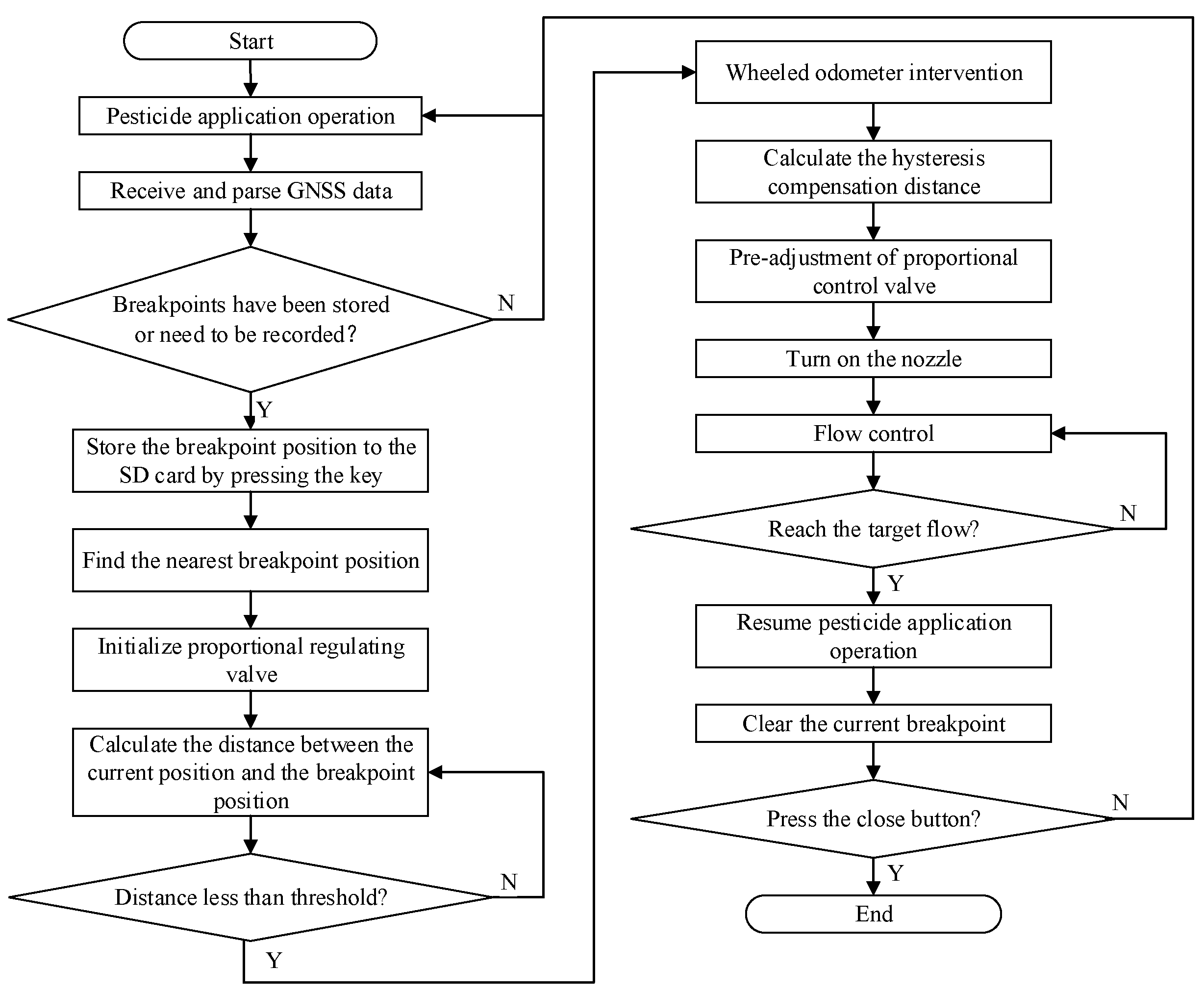
The software of the breakpoint continuous spraying system with hysteresis compensation for spraying needs to implement functions, including data acquisition of parameters, such as flow rate, vehicle speed, and position, recording, identification and distance calculation of breakpoint positions, calculation of hysteresis compensation distance, and pre-adjustment of the proportional control valve using a PID control algorithm. The main program flowchart is shown in Figure 2.

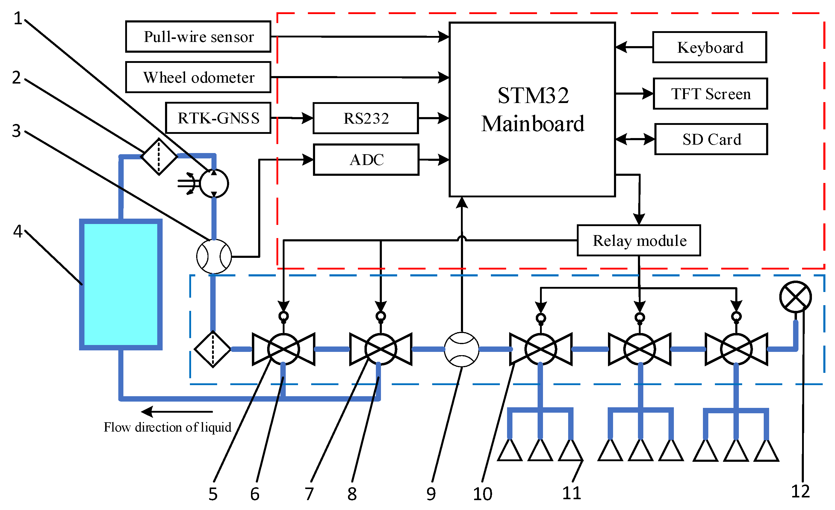
After the system startup, it parses RTK-GNSS messages to obtain UTC, longitude, and latitude, displays them on the TFT screen, and stores them in the SD card. During normal operation, the system determines if breakpoints are stored or need to be stored based on the position information. When the nearest breakpoint is detected, the proportional control valve is automatically adjusted to the initial position set by the program. Then, the real-time distance between the current position and breakpoint is calculated. When the distance is less than the threshold, the threshold is the distance at which the wheel odometer has the smallest mileage error when accumulating mileage; the wheel odometer is activated to calculate the hysteresis compensation distance required to open the nozzles. The proportional control valve is pre-adjusted to the position closest to the target flow rate, and the nozzles are opened. The PID algorithm was used to adjust the opening degree of the proportional control valve to achieve the target flow rate. Once the target flow rate is reached, normal operation resumes, and the current breakpoint information is cleared. When the main control board switch is turned off, the system shuts down.

2.2.2. PID Control Program for Pre-Adjusting the Opening Degree of the Proportional Control Valve

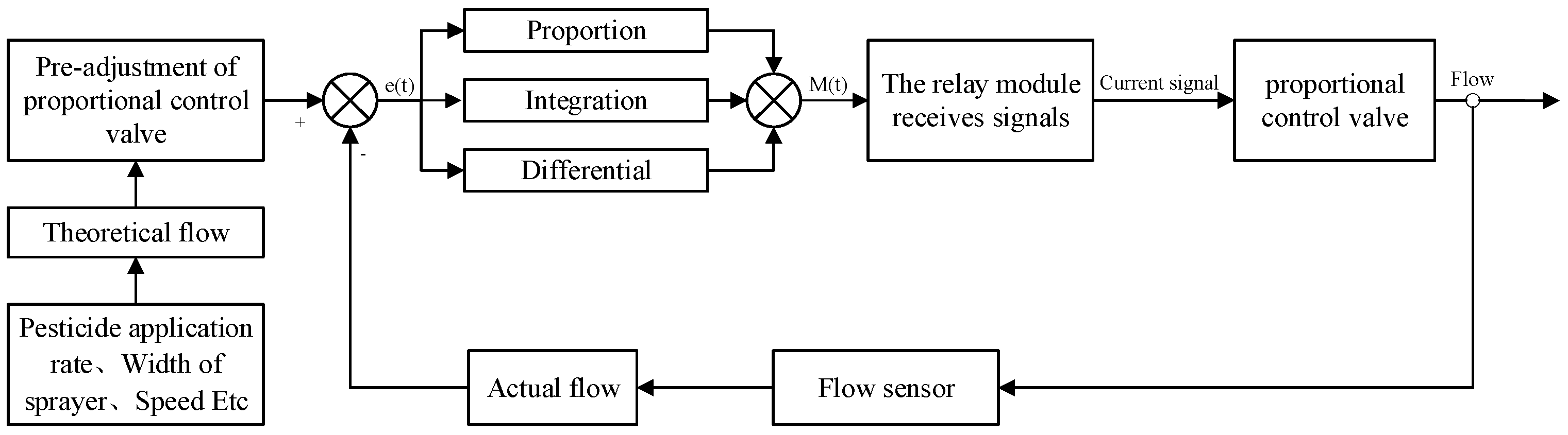
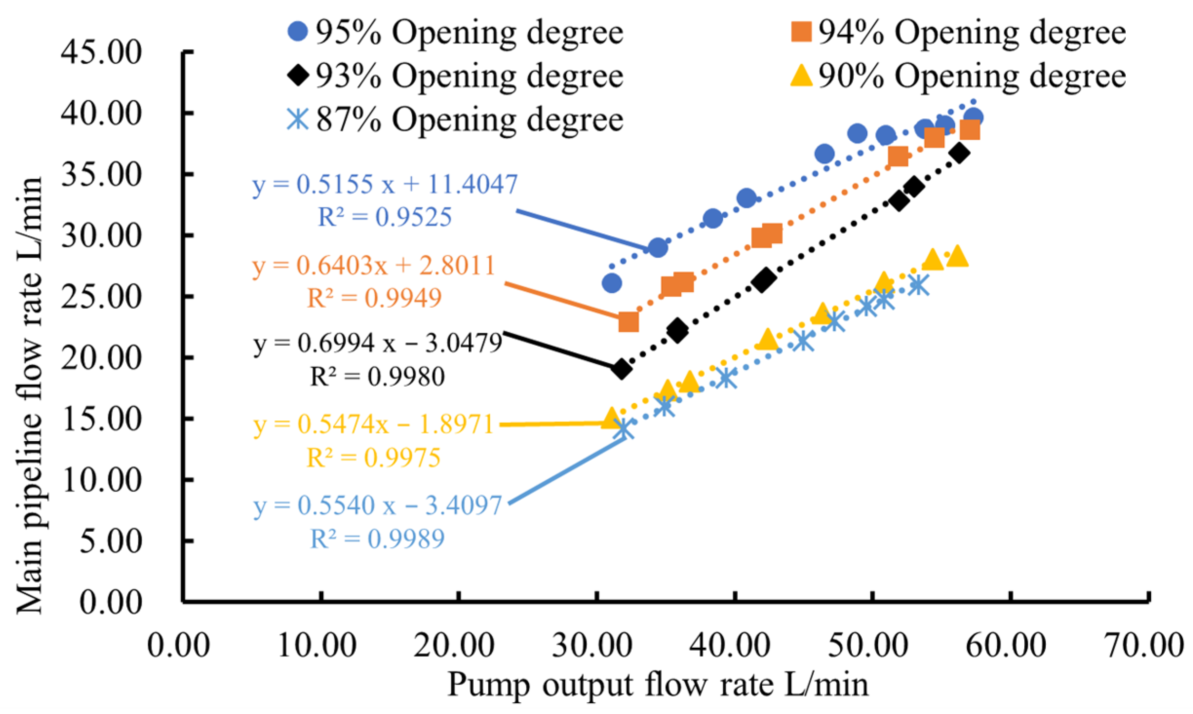
The flow control of the system uses a PID control algorithm, which pre-adjusts the opening degree of the proportional control valve to reduce the time lag in flow adjustment. First of all, the control valve opening was calibrated by resetting the control valve to a fixed initial position every time it is started, so as to ensure that the flow rate is adjusted from the same position every time. This is the process of adjusting to the initial position: the control valve to the maximum flow rate for 5 s is adjusted to ensure that the control valve has been opened to the maximum, and then it is adjusted in the opposite direction for 2 s. The opening degree of the proportional control valve was pre-adjusted by adjusting it to the opening degree closest to the target flow rate, based on the equation relating the opening degree and flow rate. Then, the actual flow rate detected within the pipeline was fed back to the controller via a flow sensor. The controller compares the actual and target flow rates and calculates the deviation signal between the two through PID calculations. This deviation signal was used to adjust the opening degree of the proportional control valve, ensuring a match between the actual and target flow rates, thus achieving closed-loop control of pesticide flow. The closed-loop control structure is illustrated in Figure 3. This method of flow rate adjustment offers advantages such as speed, stability, and accuracy [20].

The controller output of the PID controller is calculated as follows:

$$M\left(t\right)=K_p\left(e\left(t\right)+\frac{1}{T_1}{\int }_0^{t}e\left(t\right)dt+T_D\frac{de\left(t\right)}{dt}\right),$$

(1)

where

$M\left(t\right)$ is controller output;

$e\left(t\right)$ is the deviation between the target flow rate and the actual flow rate;

$K_p$ is the proportional coefficient;

$T_1$ is the integral time constant;

$T_D$ is the derivative time constant.

The controller adjusts the proportional adjustment valve according to the output value. Once discretized, the PID equation becomes

$$M\left(t\right)=K_{p}e\left(t\right)+K_i\sum _{t=0}^{k}e\left(n\right)+K_d\left(e\left(t\right)-e\left(t-1\right)\right),$$

(2)

where

$K_i$ is the integral coefficient;

$K_d$ is the derivative coefficient.

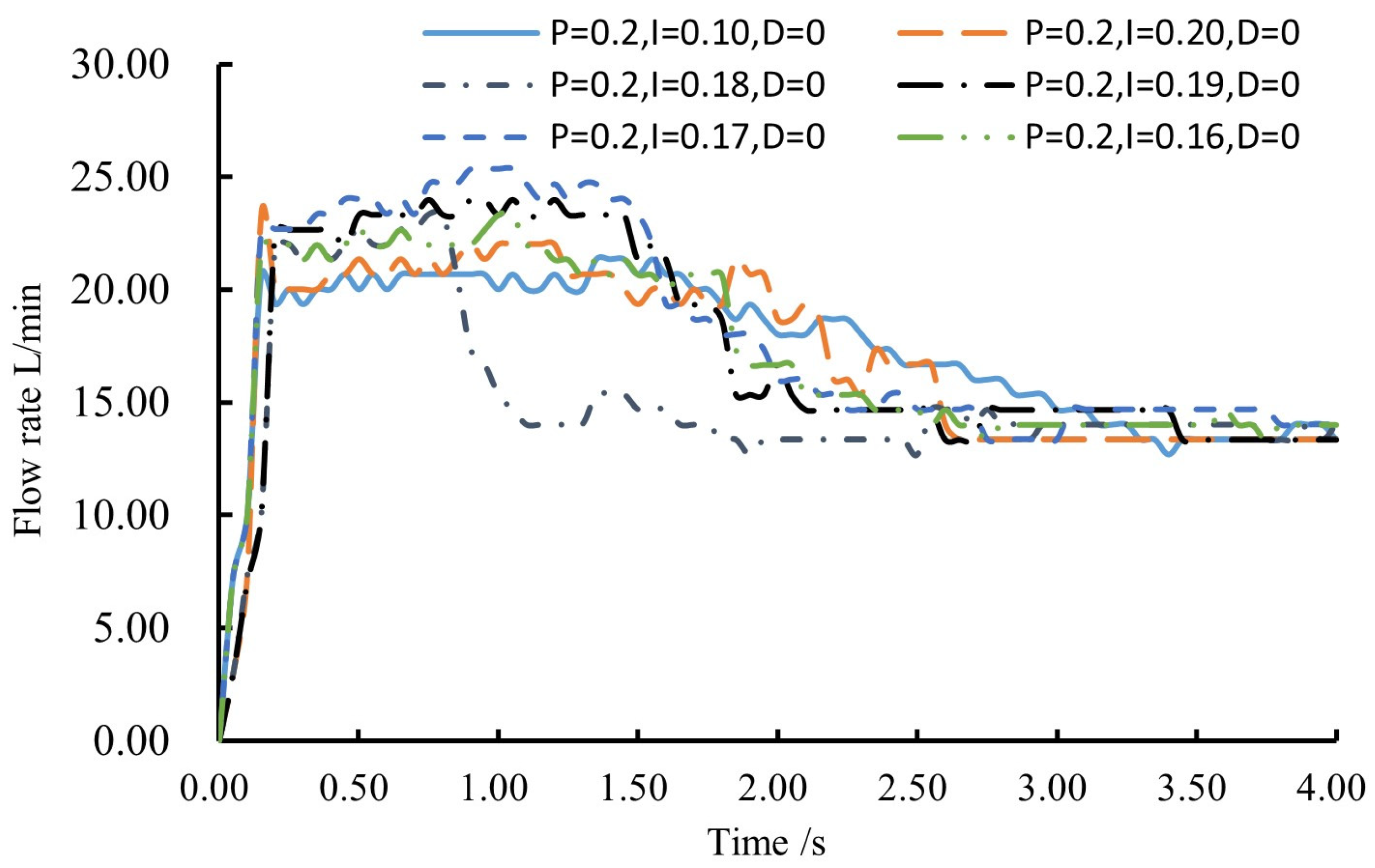
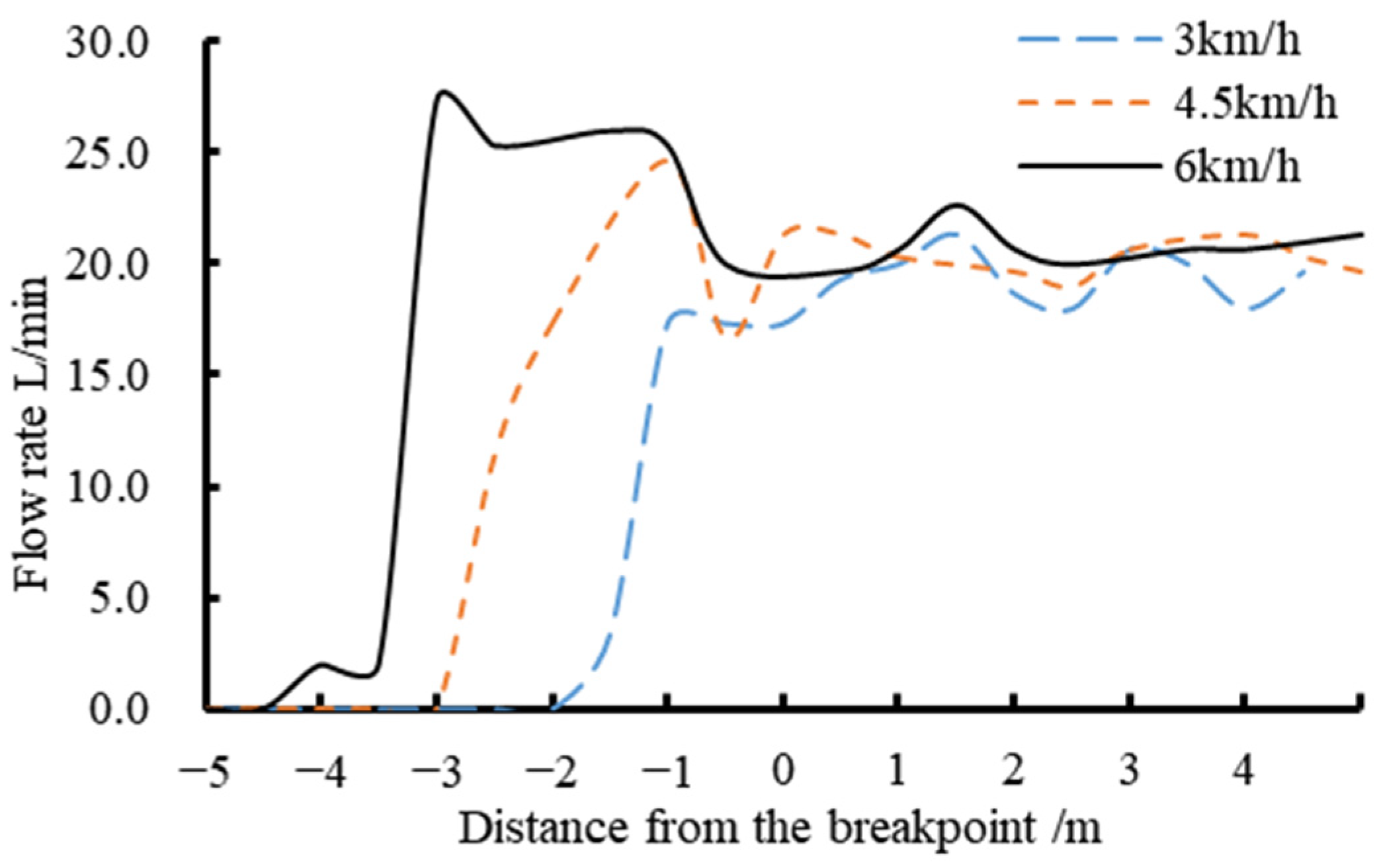
The feedback monitoring value is the main pipeline flow rate, which is affected by the vehicle speed and the rotational speed of the plunger pump, causing fluctuations during the operation process.

The main pipeline flowmeter outputs pulse signals. Its actual flow rate is calculated as

$$Q_1=\frac{60w}{k_1{t}_2},$$

(3)

where

$Q_1$ is the actual flow rate in the main pipeline, L/min;

$w$ is the number of pulses received by the controller per unit time;

$t_2$ is the time interval for flow rate detection;

$k_0$ is the flowmeter constant, taken as 90 pulses/L.

2.2.3. Hysteresis Compensation Distance Calculation Program

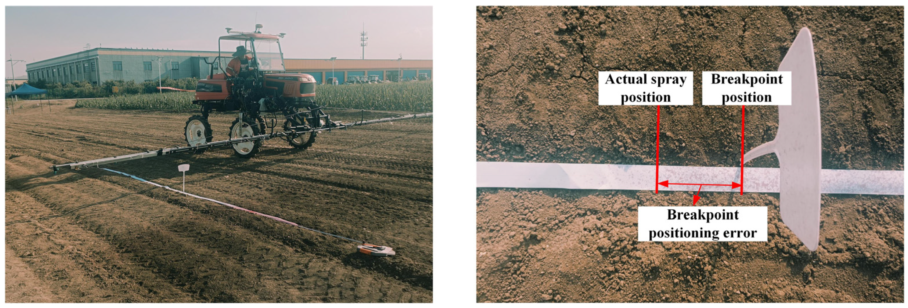
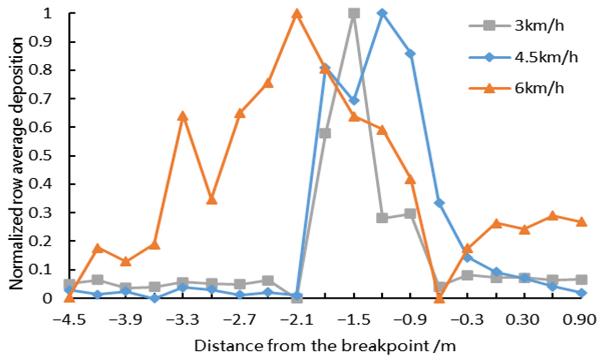
During continuous spraying, various factors, such as the time required by the switch valve to open to spray, droplet-fall time, vehicle speed, boom position, and time required to adjust the flow rate, cause the spraying and stable flow rate positions to lag behind the breakpoint position. This lag can result in repeated or missed spraying. By obtaining the aforementioned factors, calculating the position at which the valve should be opened in advance to compensate for this hysteresis in flow rate is possible.

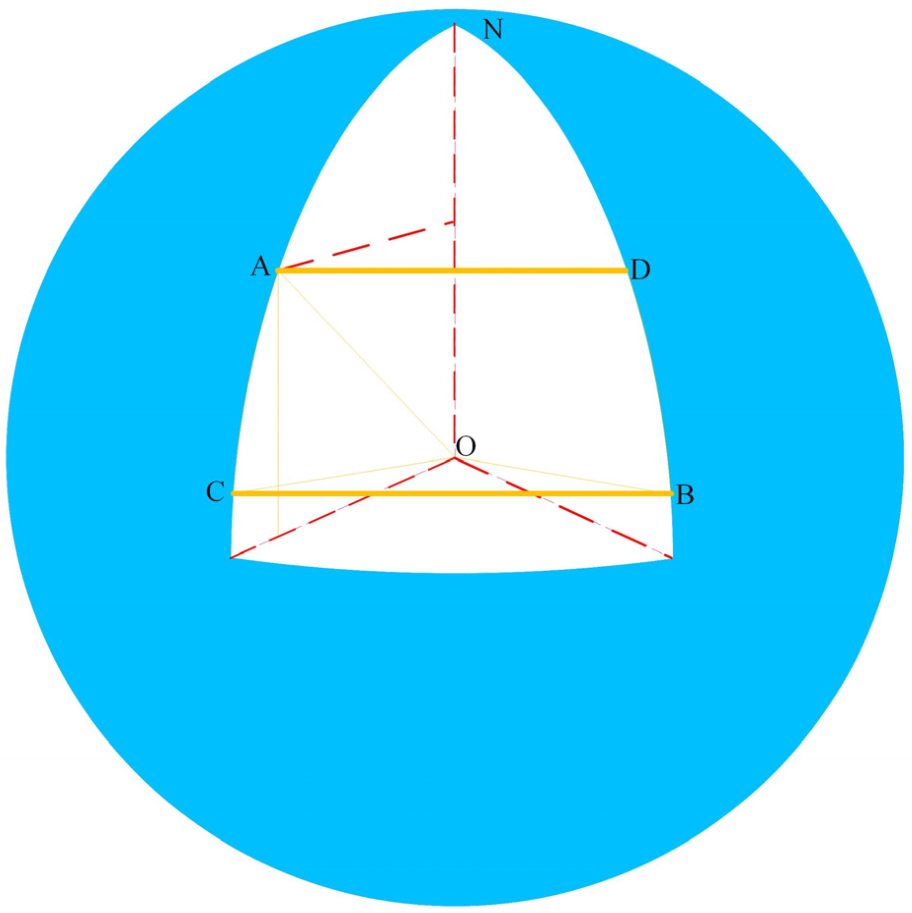
GNSS has the ability to calculate latitude and longitude automatically, but without the ability to calculate distance from one point to another point. For ease of calculation, the Earth was approximated as a sphere. The schematic diagram is shown in Figure 4. To determine the longitude and latitude ${\lambda }_1,{\phi }_1$ corresponding to points A and B, respectively, an isosceles trapezoid was constructed using points C ${\lambda }_1,{\phi }_0$ and D ${\lambda }_0,{\phi }_1$ at the same latitude as A and B. Given that ABCD is an isosceles trapezoid, the lengths of AD and CB were obtained, which helped determine the length of AB. Then, the central angle $\mathrm{\angle }AOB$ of the concentric circle with AB as the chord was calculated, yielding $\widehat{AB}$. The radian was multiplied by the radius of the Earth (R) to obtain the distance between points A and B as follows:

$$S=2\ast R\ast \arcsin \left(\sqrt{{\sin }^2(\frac{{\lambda }_0-{\lambda }_1}{2})+{\sin }^2(\frac{{\phi }_0-{\phi }_1}{2})\cos \left({\lambda }_0\right)\cos \left({\lambda }_1\right)}\right),$$

(4)

where

S is the distance between the two points, m.

When identifying breakpoints, the longitude and latitude are obtained by parsing the message on the main control board. The obtained longitude and latitude are the longitude and latitude of the RTK-GNSS installed on the boom sprayer, and the calculated S is the difference between this position and the breakpoint position.

A wheel odometer was mounted on the sprayer land wheels. By reading the number of pulse signals received within a unit of time, the traveling speed of the sprayer can be derived from known parameters, such as the wheel diameter and line count of the wheel odometer, as follows:

$$v=\frac{3.6\pi Dk}{n{t}_1},$$

(5)

where

$v$ is the travel speed;

$D$ is the diameter of land wheel, m;

$k$ is the number of pulses output by the wheel odometer in time $t_1$;

$n$ is the number of lines on the wheel odometer;

$t_1$ is the time interval for speed reading, s.

The RTK-GNSS was installed at the center of the sprayer roof, which was the located position. However, a certain distance exists between the positions of the RTK-GNSS and nozzles, and this distance changes with variations in the boom height. To establish the relationship between the RTK-GNSS and nozzle positions, the change in the length of the electric push rod was obtained through a pull-wire sensor and known lengths of the four-bar linkage. This information was then used to derive the distance relationship between the RTK-GNSS and nozzles. The structure is depicted in Figure 5.

$$L_4=L_1+\cos \left({\tan }^{-1}\left(\frac{h}{L_2}\right)\right)L_2+L_3,$$

(6)

where

$L_1$ is the distance between RTK-GNSS and the four-bar linkage, m;

$L_2$ is the length of the four-bar linkage, m;

$h$ is the height change of the four-bar linkage, m;

$L_3$ is the distance between the four-bar linkage and the nozzles, m;

$L_4$ is the distance between RTK-GNSS and the nozzles, m.

When the spray boom is 50 cm away from the ground, the actual value of $L_4$ in spraying is 1.63 m. The positioning error of RTK-GNSS data in static state is 2.5 mm + 1 ppm, and in RTK state it is 8 mm + 1 ppm. Under dynamic conditions, positioning accuracy is affected. However, as the height of the boom changes, the $L_4$ value also changes. Therefore, by monitoring the height of the boom and calculating different $L_4$ values, the positioning longitude of the nozzle position can be improved. The current position of the nozzle is the sum of S and $L_4$.

The controller calculates the cumulative mileage to be recorded based on the received mileage base, travel speed, and time required to open the nozzles as follows:

$$s=s_b+L_4-v\ast \left(t_2+t_3\right),$$

(7)

where

$s$ is the cumulative mileage recorded by the odometer, m;

$s_b$ is the mileage base, m;

$t_2$ is the time for flow rate adjustment, s;

$t_3$ is the time for nozzle opening, s.

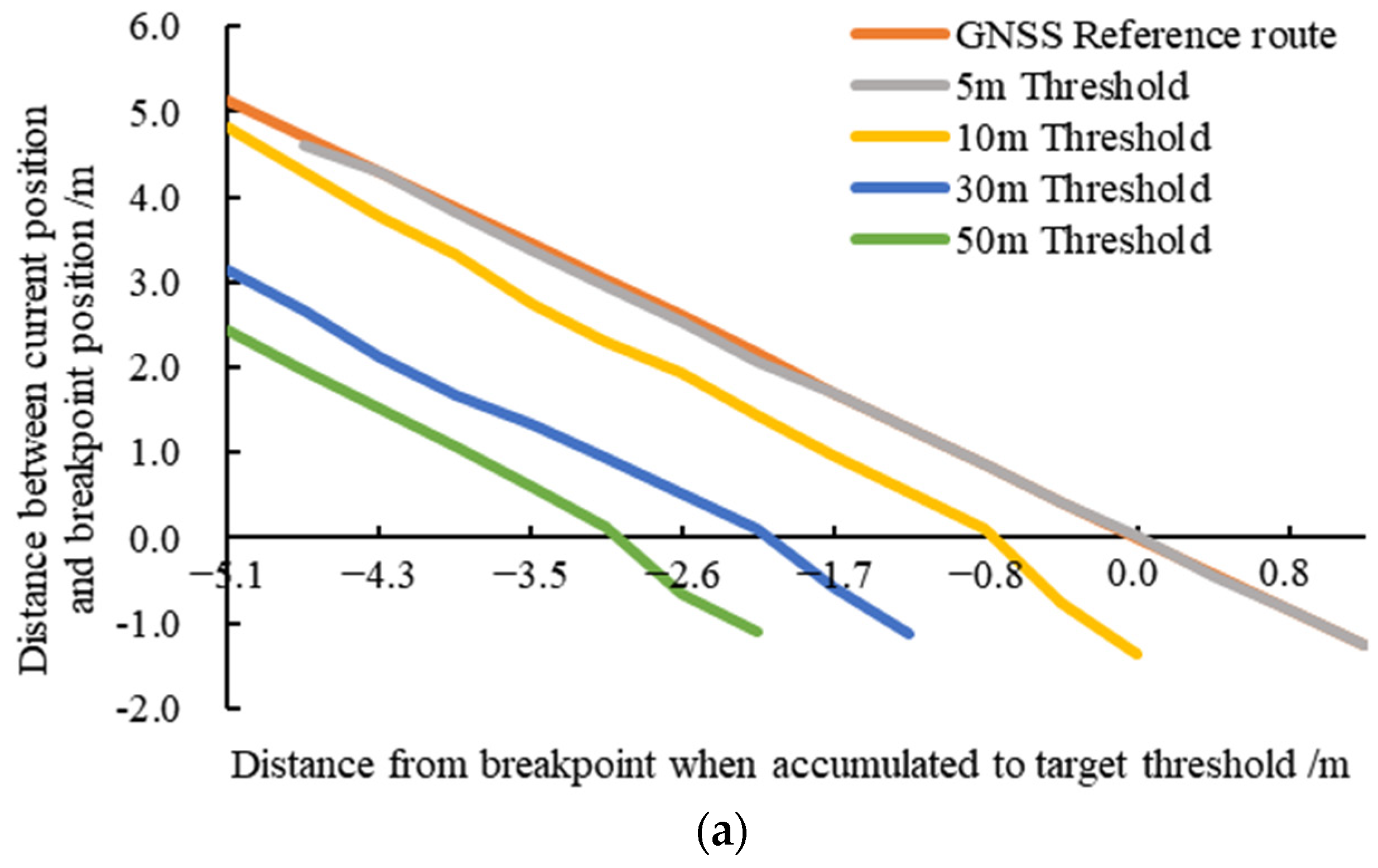
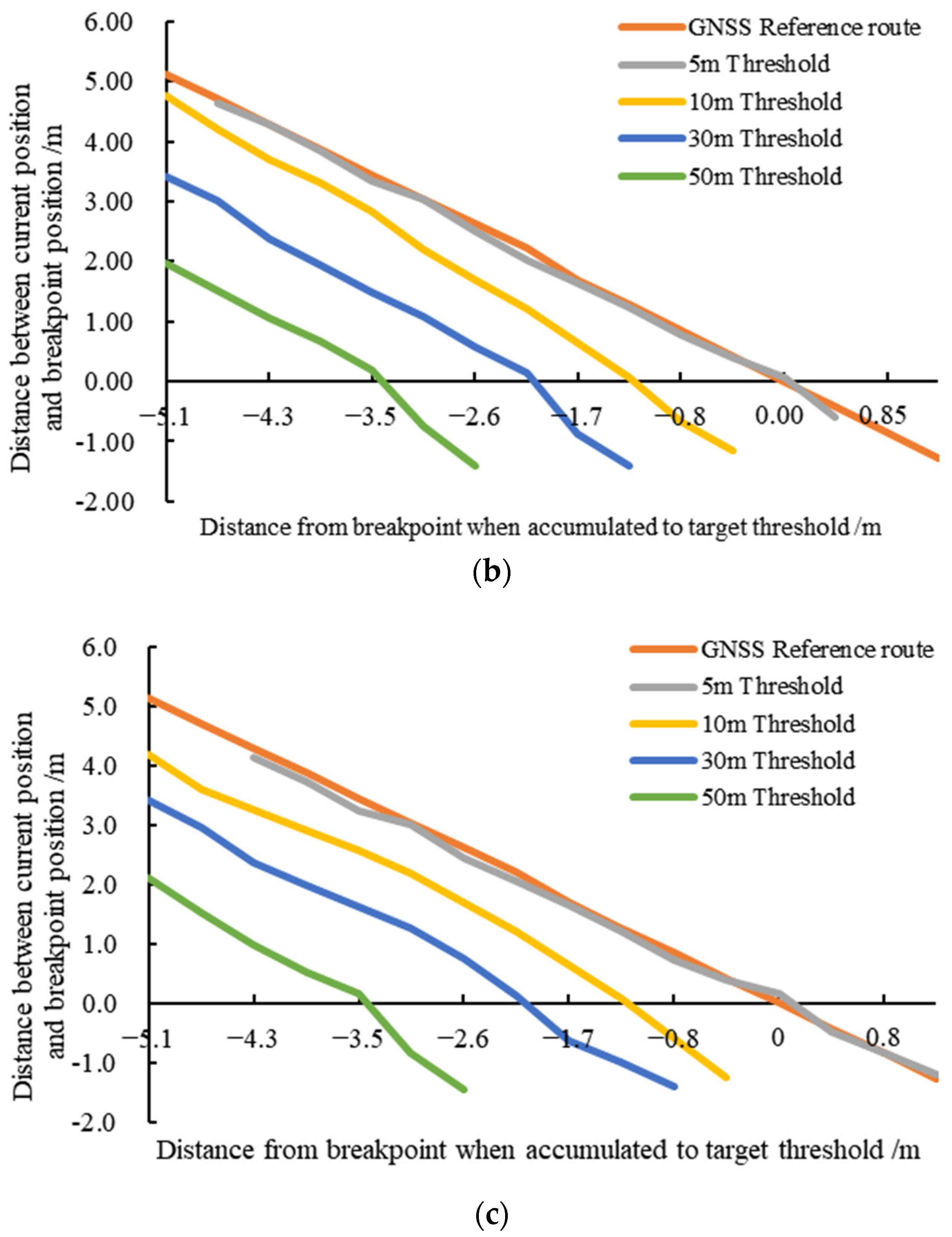
The mileage base $s_b$ is the first distance S obtained by the controller that is less than or equal to the intervention threshold of the wheel odometer. Assuming the threshold is 5 m, it is difficult to receive a longitude and latitude that is exactly 5 m away from the breakpoint due to the limitation of the RTK-GNSS update frequency. The received longitude and latitude are less than 5 m. At this time, the distance S between this longitude and latitude and the breakpoint position is the mileage base $s_b.$ The flow rate adjustment time and nozzle opening time are the main reasons for the delay in the spraying position. Therefore, the mileage base deceleration is the product of the flow rate adjustment time and nozzle opening time, and the relative position of the RTK-GNSS and the nozzle is the accumulated mileage of the wheel odometer. When this mileage is accumulated, the main control board controls the relay module to open the nozzle for continued spraying operation.

2.3. Prototype Construction

The breakpoint continuous spraying control system was designed based on the 3WSH-500 self-propelled boom sprayer (Shandong Sanhe Power Group Co., Ltd., Linyi, Shandong) The structure of the breakpoint spraying system is illustrated in Figure 6. The control system of the breakpoint continuous spraying system was centered around a SCM. The SCM receives and parses RTK-GNSS messages via the RS232 serial port, with the RTK-GNSS operating at 5 Hz. The pulse signals from the wheel odometer were received through the timer–encoder interface of the SCM, where they were converted into mileage values. The opening degree of the proportional control valve and the operation of the relief valve were controlled through the relay. The system first sets the breakpoint position and defines the A-B line for guidance. The RTK-GNSS obtains real-time position information for the sprayer. When the sprayer reaches a certain distance from the breakpoint, the wheel odometer activates and accumulates mileage data. Using high-speed imaging, the time required by the nozzles to open and start spraying and to adjust the flow rate is measured. Using a pull-wire sensor, the position at which the nozzles should be opened was determined in advance based on the distance between the nozzles and the RTK-GNSS. After the nozzles were opened, a feedforward compensation PID closed-loop control algorithm adjusted the opening degree of the proportional control valve to change the flow rate in the main pipeline. This ensured a close match between the actual and target flow rates, allowing for continuous spraying at the breakpoint position until the target flow rate was achieved.

2.4. Static Tests of Prototype

According to Equation (7), the nozzle opening and flow rate adjustment times were required to calculate hysteresis compensation distance. In this study, the nozzle opening time was acquired through high-speed imaging. Longer flow rate adjustment times resulted in larger areas of uneven pesticide deposition, leading to a decrease in spray quality. To overcome this drawback, a PID flow rate control method was proposed to pre-adjust the opening degree of the proportional control valve. In addition, the test and trial method was employed to obtain PID adjustment parameters and adjustment time.

2.4.1. High-Speed Imaging Measurement of the Time from the Output of Switch Valve Signal to Droplet Landing

The delay in pesticide application caused by the switch valve control is one of the reasons for spray hysteresis. Compensation was performed by determining the time required by the switch valve to open until the nozzles start spraying and the droplets land at different flow rates. The spray hysteresis caused by the switch valve opening until the nozzles start spraying and the droplets land at different flow rates is compensated. Initially, various opening degrees of the proportional control valve were set to alter the total pipeline flow rate. The opening degree of the proportional control valve at which all nozzles started spraying under idle conditions of the spray engine was determined. The opening degree was stepwise reduced from 90% to 1%, and observations were made to determine whether all the nozzles sprayed fully. When all nozzles failed to spray completely, the opening degree of the proportional control valve was recorded. An opening degree of ≥87% ensured full spraying of all nozzles on the spray boom. Thus, the opening degrees of the proportional control valve were set to 100%, 95%, 94%, 93%, 90%, and 87%. A GigaView series GVMC08–B05 high-speed camera (Southern Vision Systems Inc., Huntsville, AL, USA) was used to record the time required by the switch valve to open until the nozzles started spraying and the droplets landed at different flow rates. During the experiment, an LED light was parallelly connected with the switch valve control relay. It illuminated when the nozzles started spraying. The entire process of light illumination until the droplets landed was recorded. The test bench for the high-speed imaging measurement of the nozzle opening time is shown in Figure 7.

2.4.2. Tuning Test of Pump Output Flow Rate vs. Spray Flow Rate

Since the proportional control valve is a ball valve, adjusting the flow rate from the same position results in slow adjustment. A method of pre-adjusting the opening degree of the proportional control valve to reduce its flow rate adjustment time is proposed in this paper. To achieve this, the relationship between the pump output and the main pipeline spray flow rates at different opening degrees of the proportional control valve needs to be obtained. Thus, a flow sensor was added at the pump outlet to record the output flow rate of the pump. The flow sensor output current was converted into a voltage ranging from 0 to 3.3 V through a current-to-voltage module. It is calculated as

$$Q_0=\frac{50ip}{3u{k}_0}{Q}_F,$$

(8)

where

$Q_0$ is the actual flow rate at the pump outlet, L/min;

$i$ is the current output of the flow sensor;

$p$ is the range difference of the flow sensor output current;

$u$ is the range difference of the output voltage of the conversion module;

$k_0$ is the flow sensor constant, taken as 16 pulses/L;

$Q_F$ is the measurement upper limit of the flow sensor, m³/h.

The throttle size of the sprayer corresponds linearly to the output flow rate of the pump, which can be altered by changing the throttle size. Thus, the opening degree of the proportional control valve was adjusted, and the relationship between the pump output and the main pipeline flow rates was recorded for each opening degree; the pump output flow rates were set to 31.10–57.30 L/min. The relationship between the pump output and the main pipeline flow rates was recorded for each setting, and the experiment was repeated three times for each group. During data analysis, the opening degree of the proportional control valve was considered a grouping criterion, and the relationship between the pump output and the main pipeline flow rates was obtained through linear fitting for each of the five opening degrees.

2.4.3. Tuning Test of PID Parameters for Opening Degree Pre-Adjustment of the Proportional Control Valve

The PID control algorithm is the key of the PID control program for the opening degree pre-adjustment of the proportional control valve. Determination of the optimal PID control program parameters is essential. To establish the PID parameters for the said program, the values of the three coefficients of the proportional (K_P), integral (K_I), and derivative (K_D) terms were determined through the test and trial method. First, the proportional term was adjusted, and the integral and derivative terms (K_I and K_D) were set to zero, making it a pure proportional control. K_P was increased from 0.1 in increments of 0.1. Once K_P was determined, it was set to 60–70% of its determined value, and K_I was increased from 0.1 in increments of 0.05. K_P was fine-tuned according to the determined K_I. Finally, the value of K_D was determined. The time response of flow rate for various combinations was observed, and the evaluation criterion was set as a fast flow rate response without oscillation. The optimal values of PID parameters were thereby determined. Finally, the opening degrees of the proportional control valve were set to 87%, 90%, 93%, 94%, and 95%, with a target flow rate of 15–27 L/min. The adjustment time corresponding to the target flow rate was determined to validate the flow rate control performance of the algorithm.

2.5. Field Dynamic Testing

The field tests were used mainly to verify the breakpoint identification accuracy of the fusion positioning (RTK-GNSS + wheel odometer) and the flow rate control characteristics of breakpoint continuous spraying under varying vehicle speeds. The measurement of droplet deposition was conducted. The tests were conducted in early July–August 2023, in the corn cultivation area of the Xiaotangshan National Precision Agriculture Research and Demonstration Base. The meteorological conditions during the tests were as follows: Beaufort scale 1, average wind speed 1.5 m/s, temperature 36 °C, and relative humidity 76%. The pesticide sprayer has a rated pesticide tank capacity of 500 L and a spraying width of 12.2 m, and it is equipped with 22 nozzles. The selected nozzles were of the IDK 120-3 type (Lechler, Metzingen, Germany), designed to prevent drift, and had a spray angle of 90°. The spraying pressure of the nozzles was 200–500 kPa.

2.5.1. Breakpoint Identification Testing on RTK-GNSS and Wheel Odometer Fusion Positioning

The RTK-GNSS provides high positioning accuracy but exhibits a slow update rate. The positioning accuracy under static RTK is 2.5 mm + 1 ppm, and the fastest update cycle is 5 Hz. The wheel odometer accumulates large errors but has a fast update rate. Combining these characteristics, the RTK-GNSS was used to determine the distance to the breakpoint position. When the distance to the breakpoint position reached a threshold, the wheel odometer was activated to calculate the mileage. The uneven terrain of the field and engine speed variations of the sprayer may cause errors in the odometer-recorded distance compared to the actual distance. To determine the odometer-recorded distance with minimal error, a threshold determination experiment was conducted on the fusion positioning (RTK-GNSS + wheel odometer). The threshold was determined through the following process: a guidance route was set using on-board guidance, and a breakpoint coordinate was stored on this route. The sprayer returned to a position more than 50 m away from the breakpoint and gradually approached the breakpoint at a speed of 0.42 m/s along the set route. The coordinates (latitude and longitude) of this route and the distance information from the coordinates to the breakpoint coordinates were used to create a reference trajectory. Without changing the breakpoint position, threshold determination experiments were conducted at speeds of 3, 4.5, and 6 km/h, with distances of 5, 10, 30, and 50 m from the breakpoint. When the sprayer crossed the breakpoint position on the onboard guidance route, which was approximately 5 m beyond the set threshold, the cumulative mileage, coordinates, distance information of the breakpoint, and complete trajectory information were stored in the SD card. This information was then compared with the reference trajectory from the RTK-GNSS. The experimental scene of breakpoint identification and positioning accuracy is illustrated in Figure 8.

To validate the positioning accuracy of the fusion positioning and breakpoint identification algorithm, a comparative test was conducted between the RTK-GNSS + wheel odometer and the RTK-GNSS-only positionings. The test covers the following steps. First, the breakpoint position was set, colored label paper was placed 2 m before and after the breakpoint, and the breakpoint position was marked on the paper. Then, the sprayer approached the breakpoint position at speeds of 3, 4.5, and 6 km/h. Three repetitions were conducted for each speed. The distance from the red mark on the 5 cm wide colored label paper to the breakpoint was measured to compare the breakpoint identification accuracy.

2.5.2. Testing on Flow Rate Control Characteristics and Droplet Deposition Measurement of Breakpoint Continuous Spraying under the Influence of Vehicle Speed and Dosage

In this subsection, the flow-rate-control performance verification of the system during breakpoint continuous spraying with a target flow rate of 20 L/min at speeds of 3, 4.5, and 6 km/h is discussed. The three speeds corresponded to dosages of 328, 219, and 164 L/ha, respectively. During the testing, the system recorded vehicle speed, main pipeline flow rate, and distance to the breakpoint on the SD card during breakpoint continuous spraying. By analyzing the variation laws in distance to the breakpoint and the corresponding main pipeline flow rate, the hysteresis compensation and flow rate control performance of the system during breakpoint continuous spraying were validated.

Furthermore, to assess the issue of repeated and missed spraying during breakpoint continuous spraying, a test for droplet deposition was conducted under different vehicle speeds. The test scenario is depicted in Figure 9. During the test, an aqueous solution of Rhodamine B with a concentration of 0.18 g/L (Tianjin Hermel Chemical Reagent Co., Ltd., Tianjin, China) was prepared and added to the pesticide tank. Next, the unloading valve of the pesticide tank was opened for a 5 min long refluxing to ensure uniform mixing [21]. The prepared solution was diluted to five concentrations: 45, 90, 180, 360, and 720 µg/L. Calibration was performed using a Trilogy 7200-000 fluorescence analyzer (Turner Designs, St. San Jose, CA, USA). Six columns of filter papers (diameter 9 cm, Hangzhou Special Paper Co., Ltd., Hangzhou, China) were laid at intervals of 30 cm beneath the positions of sections a and c of the boom, and four columns beneath section b. The height of the boom from the filter paper is 50 cm. A total of 19 rows of filter paper was used. The sprayer was driven at speeds of 3, 4.5, and 6 km/h with a target flow rate of 20 L/min. When the actual spraying position is before the breakpoint position, there will be a section of crop that is repeatedly sprayed between the breakpoint and the actual spraying position, and the repeated spraying positions are the actual spraying position; Similarly, when the actual spraying position is after the breakpoint position, the missed spraying position is the actual spraying position.

First, the sprayer sprayed only up to the set and marked breakpoint position. Then, the sprayer returned to the starting position for continuous spraying. After setting the guidance route, the sprayer was driven toward and through the breakpoint until it crossed the area of the filter paper. Next, the filter paper with Rhodamine B solution was allowed to air-dry naturally, and then it was collected column by column. The concentration of Rhodamine B solution on each filter paper was measured using the fluorescence analyzer [22]. The coefficient of variation (CV) of droplet deposition was calculated to determine the uniformity of spray deposition [23,24,25]. The total droplet deposition in each row of the filter paper was treated as a group. According to the variation of droplet deposition in each group, 19 rows were categorized into operational, repeated spraying, and continuous spray areas. The mean, standard deviation, and CV were calculated for each area. To consider factors such as the decomposition of the solution in the pesticide tank, data were normalized to a specific range. The normalization and CV were calculated as follows:

$$y=\frac{\left(x_i-x_{min}\right)}{\left(x_{max}-x_{min}\right)},$$

(9)

$$\overline{x}=\frac{1}{n}\sum _{i=1}^n{x}_i,$$

(10)

$$S_x=\sqrt{\frac{1}{n}\sum _{i=2}^n{\left(x_i-\overline{x}\right)}^2},$$

(11)

$$CV=\frac{S_x}{\overline{x}},$$

(12)

where

$x_i$ is the sum of deposition on the i-th row of the filter paper, μg/L;

$x_{min}$ is the minimum row droplet volume during one test, μg/L;

$x_{max}$ is the maximum row droplet volume during one test, μg/L;

$y$ is the normalized row droplet volume;

$\overline{x}$ is the mean of row droplet volume in an area, μg/L;

$S_x$ is the standard deviation of row droplet volume in an area, μg/L;

$CV$ is the CV of row droplet volume in an area, %;

3. Results and Discussion

3.1. Static Testing

3.1.1. High-Speed Imaging Measurement of the Time from the Output of Switch Valve Signal to Droplet Landing

As shown in Figure 10, the moments in high-speed imaging when the LED indicator was illuminated, the nozzle started spraying, and droplets landed were recorded. The moment the LED indicator turned on corresponded to the time of the system output signal. The interval from the LED illumination to the outset of nozzle spraying represents the nozzle opening time. The time between the outset of nozzle spraying and fan-shaped droplets landing represents the droplet fall time.

The times from the system output of the switch valve signal to droplet landing are illustrated in

Table 1. High-speed imaging recording time.

Opening Degree/%	t3/s	t4/s	t5/s
100	0.200	0.270	0.070
95	0.200	0.260	0.060
94	0.200	0.260	0.060
93	0.200	0.270	0.070
90	0.200	0.260	0.060
87	0.200	0.280	0.080
Average	0.200	0.267	0.067

In the table: t₃ is the time from LED lighting to nozzle opening, s; t₄ is the time from nozzle opening to droplet landing, s; t₅ is the time from water discharge to droplet landing, s.

. Based on the experimental results, regardless of the opening degree of the proportional control valve, the time required by the nozzles to open at a distance of 50 cm from the ground remained constant at 200 ms with a standard deviation of 0.11 ms. The time from the nozzle opening to droplet landing was 0.059995–0.079994 s. The average time from nozzle opening to droplet landing was 267 ms, with a standard deviation of 7.45 ms. As the opening degree of the proportional control valve decreased, the nozzle opening time remained constant; no consistent increase or decrease was observed in the time from nozzle opening to droplet landing. Furthermore, the variation in this time was relatively small. The time difference from nozzle opening to droplet landing was relatively small at 20 ms. Therefore, the delay time from the system output signal to droplet landing was set to 267 ms. The droplet landing is primarily influenced by various factors, such as droplet size, air resistance, gravity, and environmental conditions, during the pesticide spraying operation [26]. Since the solution in the pesticide tank, vehicle speed, and environmental conditions remained relatively stable during the spraying operation, the droplet fall time was not significantly affected.

3.1.2. Tuning Test of PID Parameters for Opening Degree Pre-Adjustment of the Proportional Control Valve

The relationship between pump output and main pipeline flow rates for five different opening degrees of the proportional control valve was fitted using a primary linear regression equation, and it reflected a strong correlation, as shown in Figure 11. Specifically, for all opening degrees R² > 0.99. However, for 95% R² = 0.9525. The adjustable range of effective flow rate was from 14.20 to 38.6 L/min for the pump output flow rate of 31.10–57.30 L/min. The results indicate that as the opening degree of the proportional control valve increased while the pump output flow rate remained constant, the pesticide flow rate gradually increased. Therefore, adjusting the opening degree of the proportional control valve can control the main pipeline flow rate. However, the range of flow rate adjustment was still influenced by the pump output flow rate, the monitoring of which is crucial for adjusting the target flow rate.

Moreover, for the tuning of PID parameters, first, K_P was adjusted from 0.1 with increments of 0.1 in each iteration. Experimental results revealed that the system exhibited oscillations at K_P = 0.4, but it remained stable for 0.2 < K_P < 0.3. Thus, K_P was determined as 0.24. After setting K_P to 60% to 70% of its current value, K_I was initialized at 0.1 and incremented by 0.05. Then, the response of the main pipeline flow rate was assessed. Based on these test results, as shown in Figure 8, oscillations were absent for K_I < 0.2. After conducting tests at intervals of 0.01, K_I was determined as 0.18, and, consequently, K_P was fine-tuned to 0.20. Finally, K_D was adjusted to 0.001. The parameters obtained after multiple trials can enable a fast response without oscillation. Through repeated testing, for optimizing the system response, the values of K_P, K_I, and K_D were determined as 0.20, 0.18, and 0.001, respectively. The determination process of PID parameter K_I when K_D is 0 is illustrated in Figure 12.

Finally, the adjustment time required for the target flow rate corresponding to opening degrees of 90%, 93%, 94%, and 95% was measured. Each combination was repeated five times, and the average was calculated. The obtained flow adjustment time of the PID control for pre-adjusting the opening degree of proportional control valve is summarized in

Table 2. Flow rate adjustment time of the PID control for pre-adjusting the opening degree of proportional control valve.

Opening Degree/%	Value	Time to Adjust to Target Flow Rate/s
		27/(L·min−1)	26/(L·min−1)	25/(L·min−1)	24/(L·min−1)
95	Average	1.642	1.098	1.139	1.172
	Standard deviation	0.161	0.056	0.074	0.132
94		23/(L·min−1)	21/(L·min−1)
	Average	1.198	1.218
	Standard deviation	0.002	0.025
93		20/(L·min−1)	19/(L·min−1)	18/(L·min−1)
	Average	1.286	1.308	1.399
	Standard deviation	0.020	0.020	0.282
90		17/(L·min−1)	16/(L·min−1)	15/(L·min−1)
	Average	1.428	1.716	1.708
	Standard deviation	0.292	0.040	0.017

. Overall, under four different opening degrees of the proportional control valve, for the target flow rate of 15–27 L/min, the longest and average adjustment times were 1.716 and 1.359 s, respectively, and the standard deviation was 0.25 s. The flow rate control accuracy exhibited a minimum, average, and standard deviation values of 94.91%, 97.23%, and 1.67%, respectively.

Electric-ball-valve-based flow rate control offers the advantage of long-term reliability, and it is a primary method for adjusting pesticide flow rate in large field sprayers in the world. Notable examples include the John Deere R4030 self-propelled sprayer (Deere & Company., Moline, IL, USA), the LEMKEN Primus tractor-mounted field sprayer (LEMKEN GmbH & Co., Alpen, Germany), and the MAEC 3WZG-3000A high-clearance self-propelled boom sprayer(Modern Agricultural Equipment Co., Ltd. Beijing, China). To achieve finer proportional adjustment capability, the electric ball valve requires more time to transition from the reset to flow rate adjustment positions each time it starts, resulting in increased delay [27]. To achieve precise post-breakpoint spraying, flow rate adjustments need to be performed in advance to consider this delay. A few researchers, such as Xu et al. [14], have focused on flow rate control accuracy and succeeded in reducing the adjustment time to 3.84 s. However, they did not significantly enhance the adjustment speed of the electric ball valve from the reset position to the target flow rate. In this study, the time from closing to opening of the control valve was 11 s. By monitoring the pump output flow rate, the system controlled the movement of the electric ball valve to the optimal reset position before nozzle opening and conducted PID control parameter tuning. The adjustment time for reaching the target flow rate from nozzle start was reduced to a maximum of 1.708 s when the target flow rate was 15–27 L/min, without affecting the precision of spray flow rate. According to Formula (7), the reduction of the flow adjustment time shortens the lead spray distance, so the distance of repeated spraying will be reduced theoretically. This significantly improved the flow rate adjustment speed of the electric-ball-valve-based proportional control valve and clarified the flow rate adjustment time during breakpoint continuous spraying, which significantly contributes to reducing repeated spraying at breakpoint boundaries.

3.2. Field Dynamic Testing

3.2.1. Threshold Determination and Breakpoint Identification Accuracy Comparison Test Results on RTK-GNSS and Wheel Odometer Fusion Positioning

Figure 13 shows the breakpoint identification accuracy corresponding to the distance breakpoint thresholds recorded by the RTK-GNSS at speeds of 3, 4.5, and 6 km/h. Based on the test results, the minimum errors at speeds of 3, 4.5, and 6 km/h were 2.54, 7.22, and 15.07 cm, respectively. Across all speeds, as the threshold decreased, the error in breakpoint identification consistently decreased, with the minimum error at a threshold of 5 m. The maximum and average errors in breakpoint identification were 3.45 and 1.59 m, respectively, and the standard deviation was 1.15 m. Factors such as wheel deformation and uneven field terrain were responsible for an error between the odometer-recorded and actual mileages. This error accumulated as the recorded mileage increased, resulting in larger errors with greater recorded mileage and smaller errors with less mileage.

In addition, considering the time from valve opening to droplet landing as 0.267 s, and the flow rate adjustment time of 1.359 s, a minimum distance of 2.71 m is needed at 6 km/h to compensate for the hysteresis spraying. Thus, the threshold needs to be greater than 2.74 m. Furthermore, to ensure that the system has sufficient time for data processing and calculations, 5 m was selected as the threshold.

The accuracies of breakpoint identification, considering RTK-GNSS + wheel odometer fusion and only RTK-GNSS, are summarized in

Table 3. Breakpoint identification accuracy of RTK-GNSS and wheel-odometer fusion method.

Speed/(km·h−1)	Serial Number	Distance from Breakpoint Position/cm
3.0	1	15.85
	2	13.35
	3	12.55
4.5	4	9.25
	5	7.85
	6	8.90
6	7	5.35
	8	4.85
	9	5.65

and

Table 4. Breakpoint identification accuracy relying only on RTK-GNSS.

Speed/(km·h−1)	Serial Number	Distance from Breakpoint Position/cm
3.0	1	6.52
	2	5.32
	3	7.25
4.5	4	37.50
	5	36.25
	6	36.42
6.0	7	79.25
	8	38.25
	9	37.65

, respectively. As can be observed from Table 3 and Table 4, before fusion, the breakpoint identification distance increased with an increase in vehicle speed, with a maximum value, overall average, and standard deviation of 79.25, 31.60, and 21.97 cm, respectively. After removing the outlier at 79.25 cm, the average identification distance was 25.65 cm, with a standard deviation of 14.96 cm. Before fusion, the identification accuracy was sufficiently high at low speeds; however, it significantly deteriorated with increasing speed. This is due mainly to the limitation imposed by the update frequency of RTK-GNSS (with a maximum update rate of 5 Hz, which is equivalent to a position update interval of at least 0.2 s), leading to larger errors at higher speeds. Although an average identification distance of 31.60 cm falls within an acceptable range, RTK-GNSS may experience signal loss when receiving satellite messages, as shown in Table 4 (eighth time), resulting in a doubling of identification error. When encountering similar issues, other researchers, such as Li et al. [9], Han et al. [28], and Yin et al. [29], employed a combination of RTK-GNSS and Inertial Measurement Unit (IMU) to improve guidance accuracy and stability. Among these, the lowest average error was 1.074 cm, with a standard deviation of 1.396 cm. After fusion, the breakpoint identification distance decreased with increasing vehicle speed, with a maximum, average, and standard deviation of 15.85, 9.29, and 3.66 cm, respectively. This is because fusion captures different distances below the 5 m threshold at different speeds, resulting in smaller distances being captured at higher speeds. Thus, the distance decreased with increasing speed, with a maximum and minimum identification errors of 15.85 and 4.85 cm, respectively. The fusion method in this study, while having larger errors than the fusion approaches mentioned above, is more cost-effective and still achieves the required accuracy for field pesticide application. Therefore, the RTK-GNSS + wheel odometer fusion can effectively reduce the identification error for breakpoints.

3.2.2. Impact of Vehicle Speed on Flow Rate Control and Droplet Deposition in Breakpoint Continuous Spraying

Figure 14 depicts the flow rate control response curves at speeds of 3, 4.5, and 6 km/h, with a target flow rate of 20 L/min and corresponding dosages of 328, 219, and 164 L/ha, respectively. The average flow rates from the start of spraying until the stabilization of the flow rate are listed in

Table 5. Test results of flow rate control characteristics.

Target Flow Rate/(L·min−1)	Speed/(km·h−1)	Flow Rate/(L·min−1)	Error/%
20	3.04	19.58	−2.08
	4.55	20.47	+2.36
	5.95	20.48	+2.42

. At these three speeds, the positions at which the flow rate adjustment began were 1.70, 2.55, and 3.45 m before the breakpoint, respectively. This distance from the adjustment position to the breakpoint increased with speed as the time required by the switch valve to open to spray, droplet fall time, and the time to adjust to the target flow rate remained relatively constant. Therefore, as vehicle speed increased, the distance to the flow adjustment position also increased. The response times for flow rate control at the corresponding three speeds were 1.8, 2.2, and 1.8 s, and the corresponding flow rate errors were 2.08%, 2.36%, and 2.42%, respectively. The relative errors between the target flow rate and actual dosage were within 3%, indicating a high level of accuracy in pesticide flow rate control.

As shown in

Table 6. CV values in different areas at different speeds.

Speed/(km·h−1)	Operational Area	Average/(μg·L−1)	Standard Deviation Average/(μg·L−1)	CV/%
3.0	Operational area	7538.37	398.93	5.29
	Repeated spraying area	21,762.58	14,200.09	65.25
	Continuous spray area	8281.41	141.46	1.71
4.5	Operational area	3919.84	107.26	2.74
	Repeated spraying area	9129.98	3253.83	35.64
	Continuous spray area	4128.52	185.32	4.49
6.0	Operational area	1146.34	75.78	6.61
	Repeated spraying area	1690.81	190.93	11.29
	Continuous spray area	1231.21	2021.00	8.35

and Figure 15, the CV values for the operational and continuous spray areas ranged from 1.71% to 8.35%. Research conducted by the Prairie Agricultural Machinery Institute in Canada suggests that for CV < 10%, pesticide distribution is highly uniform. For 10% < CV < 15%, the distribution is acceptable and usable. However, for CV > 15%, the distribution model becomes impractical for field use [30,31]. This indicates that the flow rate was stable and the deposition of droplets was uniform in the operational and continuous spray areas, with stable positions occurring 0.3–0.6 m before the breakpoint. In the repeated spraying area, 11.29% < CV < 65.25%. This suggests that in the repeated spraying, the droplet overlap area leads to larger CV values, and as vehicle speed increases, the repeated spraying area expands. This may be due to smaller differences in hysteresis compensation time, which can result in an increase in repeated spraying distance with higher speeds. According to the test results, at vehicle speeds of 3, 4.5, and 6 km/h, the repeated spraying lengths were 1.5, 1.8, and 3.3 m, respectively. The repeated spraying positions were 0.6–2.1 m, 0.3–2.1 m, and 0.3–3.6 m before the breakpoint, respectively. In conclusion, according to the experimental results, the system is capable of achieving accurate and stable flow rate control within 3.6 m before the breakpoint, thus effectively eliminating instances of missed spraying. When the positions were normalized to 0.6, 2.1, and 3.6 m before the breakpoint, the normalized values became zero. At these positions, the flow rate became unstable, and the corresponding deposition was minimal in the single experiment. After normalization using Equation (9), the calculated results became zero. A few researchers, such as Wen et al. [32] and Lipiński et al. [33], primarily assessed spray uniformity using the CV for evaluating droplet deposition uniformity with Rhodamine B solution. They did not specifically evaluate the repeated and missed spraying performance during breakpoint continuous spraying using CV. This study combined initial spray flow rate adjustment with breakpoint continuous spraying to enhance breakpoint identification accuracy. Thus, hysteresis compensation for spraying was introduced to entirely eliminate the missed spraying area and to reduce the repeated spraying area to 39.04 m². The repeated spraying area is the product of sprayer boom width and repeated spraying lengths, The proposed approach could reduce even more repeated spraying area in sprayers with wider booms. In addition to the continuous traveling of the sprayer, the autonomous operation capability of boom sprayers could be further enhanced by controlling nozzles and boom heights.

4. Conclusions

(1) A breakpoint continuous spraying system based on hysteresis compensation was designed for the 3WSH-500 self-propelled boom sprayer. Furthermore, a fusion positioning algorithm consisting of a RTK-GNSS and a wheel odometer was designed, and a PID control algorithm was devised to pre-adjust the opening degree of the proportional control valve based on the relationship between the opening degree of the spraying control valve group, pump outlet flow rate, and main pipeline flow rate. Thus, the proposed system achieved breakpoint position storage and identification, dynamic hysteresis compensation for spraying, and flow rate control.

(2) Comparative experiments were conducted to evaluate the accuracy of breakpoint identification between the RTK-GNSS + wheel odometer fusion and only RTK-GNSS positionings. The experiments were conducted at speeds of 3, 4.5, and 6 km/h. The results showed that the fusion positioning had an accuracy of 25.65 cm before fusion and 9.29 cm after fusion. Importantly, it eliminated cases where the breakpoint could not be recognized due to signal instability in RTK-GNSS, thus improving stability.

(3) Static tests were conducted to determine the time required by the switch valve to open to spray, droplet fall time, relationship between the opening degree of the spraying control valve group, pump outlet flow rate, main pipeline flow rate, PID control program parameters, and flow adjustment time. This achieved dynamic hysteresis compensation for spraying, with an average compensation time of 1.359 s. Dynamic tests confirmed the effectiveness of dynamic hysteresis compensation for spraying, demonstrating that the system could maintain the target flow rate stably within 0.3 m before the breakpoint, with a flow adjustment error of less than 3% for the target flow rate of 20 L/min and vehicle speed of 3, 4.5, or 6 km/h.

(4) Breakpoint continuous spraying experiments were conducted to measure droplet deposition under the influence of vehicle speed and pesticide dosage. By analyzing the CV of the total deposition in each row, the entire region was divided into operational, repeated spraying, and continuous spray areas. The repeated spraying distance was 1.5–3.3 m at speeds of 3, 4.5, and 6 km/h, respectively. That is, at least 3.3 m was reserved in front of the breakpoint. Thus, the proposed approach can effectively eliminate missed spraying during the breakpoint continuous spraying by the sprayer.