Review of Discrete Element Method Simulations of Soil Tillage and Furrow Opening

Abstract

In agricultural machinery design and optimization, the discrete element method (DEM) has played a major role due to its ability to speed up the design and manufacturing process by reducing multiple prototyping, testing, and evaluation under experimental conditions. In the field of soil dynamics, DEM has been mainly applied in the design and optimization of soil-engaging tools, especially tillage tools and furrow openers. This numerical method is able to capture the dynamic and bulk behaviour of soils and soil–tool interactions. This review focused on the various aspects of the application of DEM in the simulation of tillage and furrow opening for tool design optimization. Different contact models, particle sizes and shapes, and calibration techniques for determining input parameters for tillage and furrow opening research have been reviewed. Discrete element method predictions of furrow profiles, disturbed soil surface profiles, soil failure, loosening, disturbance parameters, reaction forces, and the various types of soils modelled with DEM have also been highlighted. This pool of information consolidates existing working approaches used in prior studies and helps to identify knowledge gaps which, if addressed, will advance the current soil dynamics modelling capability.

1. Introduction

In mechanized agriculture, the energy use for soil tillage operations can be as high as 50% of the total energy used in crop production [1,2]. The energy-use efficiency associated with tillage can be increased by improving the design of tillage implements and through their correct operation and settings [3,4,5]. The design optimization of tillage tools and furrow openers conventionally relies on repeated prototyping and evaluation through soil bins and field experimentation. This task is laborious, time-consuming, and expensive [6,7]. In order to reduce the resource intensity involved, various analytical and numerical models for predicting soil–tool interaction and soil forces have been developed. Analytical models are typically based on the universal earthmoving equation (Equation (1)) [8,9].

P = (γd²N_γ + cdN_c + c_adN_a + qdN_q)w

(1)

where P is soil cutting force (N), γ is the specific weight of soil (N m⁻³), d is working depth (m), c is soil cohesion (Pa), c_a is soil–metal adhesion (Pa), q is surcharge stress (Pa), w is tool width (m), and N_γ, N_c, N_a, and N_q are dimensionless N factors that are dependent on gravity, cohesion, adhesion, and surcharge, respectively.

Analytical models require a preliminary assumption of soil failure patterns to predict soil and implement forces [10,11]. These models use simple and approximate geometric profiles such as wedges and crescents that are easily expressed mathematically to model soil failure patterns [4,8,9,12,13]. They also aim to predict the maximum soil reaction force at incipient soil failure, rather than the average soil forces during the tillage process. However, in practice, soil failure occurs in more complex patterns. Analytical models also regard soil failure as bulk soil movement without accounting for interactions between individual soil particles, aggregates, and macro-organic matter evident in field conditions [7].

Numerical models, such as finite element modelling (FEM) and computational fluid dynamics (CFD), have also been employed to predict soil failure patterns and soil forces with some degree of accuracy [14,15]. However, their use is limited because they consider soil as a continuum body rather than being made up of discrete particles. Thus, continuum numerical models fail to account for variations in soil structure, physical conditions, flow, and the mixing and translocation of soil particles [6]. To overcome the shortcomings of analytical and continuum numerical methods, the discrete element method (DEM) can be employed. DEM is a discontinuum numerical method used for modelling the mechanical behaviour of granular materials. Initially developed by Cundall and Strack [16], DEM is used to model particle interactions within granular materials such as gravel, grain, soil, and powder. Unlike analytical and other numerical (continuum) approaches, DEM accounts for the discrete nature of granular particles and their interactions with neighbouring particles and interfacing objects such as contact walls and machine parts. The DEM approach involves the dynamic creation and breaking of bonds between contacting particles [7,16] and can simulate soil–tool reaction forces, as well as track particle movements and model mixing and translocating processes.

Several studies have shown that DEM can be successfully employed to model 2- and 3-dimensional space interactions between granular particles and machine parts. Operations such as grain flow in a hopper, soil movement in bulldozing, and soil deformation and displacement during field traffic, tillage and furrow opening processes have been modelled in DEM, achieving results that closely agree with experimental observations [17,18,19,20,21]. Figure 1 shows a comparison between a tine furrow opener interaction with soil (left) and its simulation with DEM (right) [21]. Other applications of DEM include modelling of cohesionless and cohesive/adhesive particles [10,18,20]. Discontinuum approaches such as DEM offer greater potential for more accurate prediction of soil–tool interactions in soil dynamics applications compared with continuum approaches. Thus, DEM is a powerful tool that can accurately guide and speed-up the design optimization process by researchers, developers, and manufacturers.

The objective of the work reported in this article was to review the various aspects of the application of DEM in the field of soil dynamics by focusing on soil tillage and furrow opening research for tool performance optimization. Contact models for soil particles; DEM particle size and shape considerations; calibration techniques for determining accurate input parameters; predictions of soil failure, particle movement and reaction forces; and the types of soils modelled with DEM have been reviewed. Knowledge gaps that need attention in future research, and that will go some way to advance soil dynamics modelling capability, have also been identified.

2. Modelling Agricultural Soils with DEM

The discrete element method is used to model soil as a collection of a finite number of individual spherical particles that interact with neighbouring particles and machine parts when subjected to external forces and forced displacement at the soil–tool interface, such as from a soil tillage tool [7]. This process induces the relative motion of particles within the bulk. Contact forces between these particles and their resultant motion are calculated using Newton’s Second Law [22]. These calculations involve repeating the same algorithm at each time step of the simulation process, using results from previous calculations as input.

2.1. DEM Contact Models

DEM contact models are developed to describe the mechanical and physical interactions of granular particles with neighbouring particles or external objects. The interactions are modelled using equations of motion and contact models expressed as linear, adhesive, and elastoplastic normal contact models, as well as viscosity, tangential force, and torque models. The tangential force and torque models account for friction, rolling, and torsion [23,24]. Physical interactions between particles are expressed via combining functional elements of springs, dampers, and tangential friction. Total contact forces are expressed as the sum of spring (F^s) and damping (F^d) forces. Some commonly used contact models in DEM simulations are listed in

Table 1. Discrete element method contact models, their advantages and disadvantages, types of soil modelled, and software used.

Contact Model	Advantages	Disadvantages	Types of Soil Modelled	References	Software Used by Researchers
Linear spring contact model	Simple to use.	Does not account for nonlinearity in loading and unloading cycles and plastic deformation of soil.	Sandy	Tanaka et al. [27], Asaf et al. [10], Shmulevich et al. [6], Ono et al. [28]	PFC2D, EDEM
Linear spring contact model with cohesion	Allows users to consider cohesion in the linear spring contact model.	Only considers the cohesion through the normal direction.	Vertosol	Bravo et al. [18]	DEMeter++
Hertz–Mindlin contact model	Simple to use. Although this model was designed for fine, dry particles, it can be used to model wet particles as well.	Inaccurate prediction for vertical tillage force.	Sandy	Ucgul et al. [29]	EDEM
Parallel bond model (PBM) or Hertz–Mindlin contact model with cohesion	Allows users to model cohesion.	Excessive forces cause the bonds to be broken irrationally.	Coarse sand, loamy, sandy loam, loessal, clay, sandy clay loam, loamy clay	Tamas et al. [30], Chen et al. [7], Bo et al. [31], Hang et al. [32], Cheng et al. [33], Yang et al. [34], Hoseinian et al. [35]	EDEM PFC3D
Hertz–Mindlin contact model with Johnson–Kendall–Roberts (JKR)	Enables the modelling of strongly adhesive bonds such as exist in dry powders or wet materials.	-	Clay, silty clay loam	Cheng et al. [33], Du et al. [36], Zhai et al. [37]	EDEM
Hysteric spring contact model	Accounts for plastic deformation during loading and unloading of soil. Suitable for both cohesive cohesionless soils.	It requires a large number of input parameters, making its setup and calibration complex.	Sandy	Ucgul et al. [38], Ucgul et al. [29]	EDEM
Hysteric spring contact model with linear cohesion contact model	Allow users to consider cohesion in the hysteretic spring contact model.	Only considers the cohesion through the normal direction.	Sandy loam, clay (Vertosol)	Barr et al. [21], Barr et al. [39], Makange et al. [40], Aikins et al. [41], Awuah et al. [42], Wang et al. [43]	EDEM
Edinburgh elasto-plastic adhesion model	It is versatile since it can be used as a linear or non-linear Hertzian spring model. It also allows tensile forces to develop and a non-linear force-displacement behaviour in compression.	It requires a lot of input parameters.	Clay, clay loam, sandy loam, loam, sandy	Kim et al. [44], Wu et al. [45], Zhao et al. [46], Sun et al. [47]	EDEM, PFC3D, LiGGGHTS

and reviewed below. These contact models have been implemented in commercially available software such as Bulk Flow Analyst™, Chute Analyst™, Chute Maven^®, DEMpack™, Altair^® EDEM™, ELFEN, GROMOS-96, ITASCA PFC (2D & 3D), LiGGGHTS^®, MIMES, PASSAGE/DEM, Rocky, SimPARTIX^®, StarCCM+, UDEC, 3DEC, and YADE [25,26]. Table 1 also shows the various DEM software that have been used in tillage and furrow opening research and the types of soil the contact models have been used to model.

The movement of particles due to the contact forces are governed by Newton’s equation of motion for linear and angular motion as expressed by Equations (2) and (3). By solving these equations, the motion of the particles can be determined. For two spherical particles (i = 1,2) of masses m_i and radii r_i, located at x_i in contact, taking F as contact force, g as acceleration due to gravity, I_i as the moment of inertia of a particle, ω_i as the angular velocity of a particle, and T_i as torque due to the tangential component of the contact force:

$$m_i{\ddot{x}}_i=F_i+m_{i}g$$

(2)

$$I_i{\dot{\omega }}_i=T_i$$

(3)

2.1.1. Linear Spring Contact Model

This contact model is linearly elastic and is the simplest contact model often used to simulate soil–tool interactions (Table 1) [6,27]. A contact force is created between the two spherical particles in contact as described above. The contact force can be decomposed into normal and tangential force components. The overlap at the contact point generates a repulsive contact force and energy dissipation. When an overlap ${\delta }_n>0$ is formed between the two particles at a relative velocity ${\dot{\delta }}_n$ in a direction normal to the contact surface, a normal contact force $F_n$ is created based on the spring and dashpot models (Figure 2) such that:

$$F_n=k_n{\delta }_n+d_n{\dot{\delta }}_n$$

(4)

The parameter k_n is the normal stiffness, while d_n is the damping coefficient. Considering an imaginary rod of radius $r=\left(r_1+r_2\right)/2$ between the centres of the two particles and Young’s Modulus E:

$$F_n=\pi Er/2$$

(5)

When the tangential component of the contact force, $F_t>{\mu }_t{F}_n$, sliding friction occurs. The local friction coefficient ${\mu }_t=tan\varnothing$, where $\varnothing$ is the internal friction angle between the particles.

The tangential component of the contact force is also given by:

$$F_t=-k_t{\delta }_t-d_t{\dot{\delta }}_t$$

(6)

where k_t, ${\delta }_t$, d_t, and ${\dot{\delta }}_t$ are tangential components of stiffness, overlap, damping coefficient, and relative velocity.

2.1.2. Hertz–Mindlin Contact Model

The Hertz–Mindlin contact model (HMCM), especially when it is used with the parallel bond model (PBM, see Section 2.1.4), is the most popular contact model used by researchers [7,30,33,34,35,48] to simulate soil–tool interaction in tillage research. However, as an (non-linear) elastic contact model, it fails to predict vertical soil forces accurately (Table 1) [49]. In this model, the contact force consists of a non-linear Hertz component described by the hysteretic spring force-displacement relationship shown in Figure 3 and a damping component (second part of Equation (7)). It is also resolved into normal and tangential components. The HMCM and its parameters are described in Equation (7) to (16) [20,29].

Normal contact force, F_n:

$$F_n=-k_n{\delta }_n^{3/2}-d_n{\delta }_n^{1/4}{\dot{\delta }}_n$$

(7)

$$k_n=2E_{eq}\sqrt{r_{eq}{\delta }_n}$$

(8)

$$d_n=\frac{\ln e}{\sqrt{{\ln }^{2}e+{\pi }^2}}\sqrt{k_n{m}_{eq}}$$

(9)

where:

Equivalent radius,

$$r_{eq}={\left(\frac{1}{r_1}+\frac{1}{r_2}\right)}^{-1}$$

(10)

Equivalent Young’s modulus,

$$E_{eq}={\left(\frac{1-{\nu }_1^2}{E_1}+\frac{1-{\nu }_1^2}{E_2}\right)}^{-1}$$

(11)

Equivalent particle mass,

$$m_{eq}={\left(\frac{1}{m_1}+\frac{1}{m_2}\right)}^{-1}$$

(12)

Tangential contact force, F_t:

$$F_t=-k_t{\delta }_t-d_t{\delta }_t^{1/4}{\dot{\delta }}_t$$

(13)

$$k_t=8G_{eq}\sqrt{r_{eq}{\delta }_n}$$

(14)

$$d_t=\frac{\ln e}{\sqrt{{\ln }^{2}e+{\pi }^2}}\sqrt{k_t{m}_{eq}}$$

(15)

Equivalent shear modulus,

$$G_{eq}={\left(\frac{2-{\nu }_1}{G_1}+\frac{2-{\nu }_2}{G_2}\right)}^{-1}$$

(16)

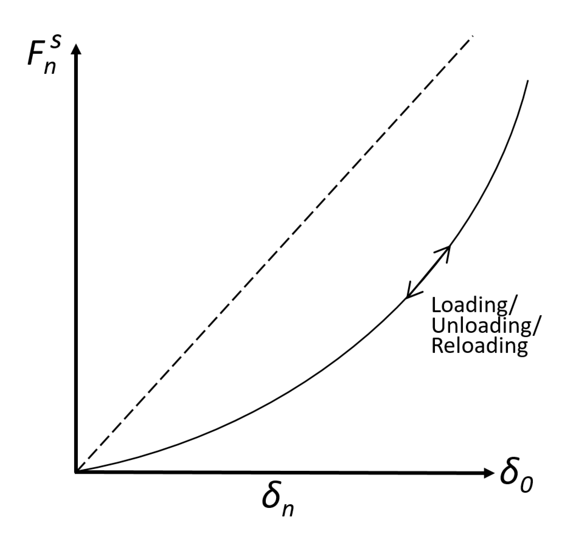
2.1.3. Hysteretic Spring Contract Model

The hysteretic spring contact model (HSCM) is an elastic–plastic contact model that accounts for the plastic deformation that occurs during the loading and unloading of soil. It makes the particles behave as though they undergo plastic deformation after the load reaches a yield point, as shown in Figure 4 [50]. The main disadvantage of this contact model is that it requires a large number of input parameters, making its setup and calibration of DEM material properties complex (Table 1) [49]. The HSCM comprises two parts: the spring characteristic illustrated in Figure 2 and damping. A comparative study by Ucgul et al. [29] revealed that the HSCM could model soil–tool interaction more accurately than the HMCM. The HSCM has been used to predict soil reaction forces as well as furrow profiles successfully, especially with the linear cohesion model [39,40,41,43]. The governing equations of the HSCM are described in Equation (17) to (20).

Normal contact force, F_n:

During loading,

$$F_n=-k_1{\delta }_n-n_c\sqrt{\frac{4m_{eq}{k}_1}{1+{\left(\frac{\pi }{\ln e}\right)}^2}}·{\dot{\delta }}_n$$

(17)

During unloading and reloading,

$$F_n=-k_2\left({\delta }_n-{\delta }_0\right)-n_c\sqrt{\frac{4m_{eq}{k}_1}{1+{\left(\frac{\pi }{\ln e}\right)}^2}}·{\dot{\delta }}_n$$

(18)

During unloading again,

$$F_n=0-n_c\sqrt{\frac{4m_{eq}{k}_1}{1+{\left(\frac{\pi }{\ln e}\right)}^2}}·{\dot{\delta }}_n$$

(19)

where k₁ and k₂ are the loading and the unloading stiffnesses, respectively, and e is the coefficient of restitution of the particles, and they are related as $e=\sqrt{k_1/k_2}$.

Tangential contact force, F_t:

$$F_t=-n_k{k}_1{\delta }_t-\sqrt{\frac{4m_{eq}{n}_k{k}_1}{1+{\left(\frac{\pi }{\ln e}\right)}^2}}·{\dot{\delta }}_t$$

(20)

where n_k is the stiffness factor equal to the tangential stiffness ratio to normal loading stiffness.

2.1.4. Accounting for Cohesion with DEM Contact Models

In reality, agricultural soils exhibit varying levels of cohesion between particles and adhesion to walls and tools they come in contact with. Attractive pressure (that is, cohesive and adhesive forces) are induced due to the capillary effect and water bridge that exists between particles in unsaturated soils [25,51,52]. Thus, a more realistic contact model for agricultural soils should account for cohesion and adhesion. The linear cohesion and parallel bond models have been used in the DEM modelling of agricultural soils (Table 1).

Linear Cohesion Model

When this model is used, a cohesive or adhesive force is added to the normal force component of the contact model used for cohesionless soils. Even though the linear cohesion model itself does not include a tangential component, its addition increases the normal force, which consequently increases frictional force for greater resistance to slippage [41,50,52,53]. The linear cohesion model can be added to any of the three contact models discussed in Section 2.1.1 to Section 2.1.3 above [50]. If F_ca (Equation (21)) is the cohesive or adhesive force, then the normal contact force is modified, as shown in Equation (22).

$$F_{ca}=r_c^2\pi \widehat{c}$$

(21)

$$F_n=F_n^s+F_n^d+F_{ca}$$

(22)

$$r_c={\left(\frac{3r_{eq}{F}_n^s}{4E_{eq}}\right)}^{\frac{1}{3}}$$

(23)

The parameter r_c is the contact radius between particles and can be determined using Equation (23). Equation (21) is called the constant cohesion model because the cohesive stress $\widehat{c}$ is a constant. The constant cohesion model makes the model particles too sticky [52]. A modification has therefore been proposed, depending on the degree of compression between two adjacent particles. If compression between two adjacent particles is given by Equation (24), then the cohesive stress increases with time t according to Equation (25).

$${\sigma }_n=\frac{F_n}{\pi r_c^2}$$

(24)

$${\widehat{c}}^{\left(t=n\right)}=k_c\underset{}{\max }\left({\sigma }_n^{\left(t=1\right)}, {\sigma }_n^{\left(t=2\right)},\dots ..{\sigma }_n^{\left(t=n-1\right)}\right)$$

(25)

Parallel Bond Model

An adaptation of the Hertz–Mindlin contact model (HMCM) for cohesive soils is the parallel bond model (PBM) developed by Potyondy and Cundall [54]. The PBM, based on beam theory, uses rectangular (2D) or cylindrical (3D) cement entities as parallel bonds at the point of contact between the two cohesive particles (Figure 5). This bond is modelled as an elastic beam whose length approaches zero and could be represented by a set of springs uniformly distributed over the contact plane and centred at the contact point [54]. After bond formation, normal and tangential bond forces and moment are calculated in addition to contact forces [50,55,56]. Thus, the bond can withstand or transmit both forces and moments between particles. The bond breaks when its predefined maximum normal or shear strengths are exceeded [57,58]. When no bond exists between particles, the PBM reverts to the HMCM [26]. The PBM is able to model clod formation and the brittle nature of agricultural soils in a more realistic manner [30,59]. It can be used only for particle-particle bonding, not particle-wall (tool) bonding [30,50]. The PBM is the most used model in cohesive soil tillage research [7,30,31,51,55,56,57,58,59,60,61,62,63,64,65,66,67,68,69,70]. Because the base contact model of the PBM is the HMCM, it also fails to predict vertical soil forces accurately as revealed in Table 2 [55,69]. Details of the PBM can be found in Potyondy and Cundall [54].

Johnson–Kendall–Roberts Cohesion

Another cohesion contact model combined with the HMCM is the Johnson–Kendall–Roberts (JKR) cohesion model [71]. It has been used by researchers such as Cheng et al. [33], Du et al. [36], and Zhai et al. [37] to model cohesive soils in soil tillage simulations with DEM (Table 1). Using this model, the tangential contact force and the normal and tangential damping forces of the HMCM are maintained, while the normal contact force is modified to include cohesion [36]. This modification enables the modelling of strongly adhesive bonds such as exist in dry powders or wet materials (e.g., wet soil). It captures the influence of Van der Waals forces due to contact between two surfaces [50]. A cohesion or adhesion parameter called surface energy is introduced. When this surface energy is zero, the model reverts to the HMCM. The normal contact force in HMCM-JKR is given by Equations (26) and (27), as follows:

$$F_n=\frac{4E_{eq}{a}^3}{3R_{eq}}-4\sqrt{\pi \gamma E_{eq}{a}^3}$$

(26)

$${\delta }_n=\frac{a^2}{R_{eq}}-2\sqrt{\frac{\pi \gamma a}{E_{eq}}}$$

(27)

where a is JKR contact radius and γ is surface energy (J/m²).

Table 2. Relative errors in DEM-predicted soil–tool reaction forces, travel speeds, and operating depths reported in the various literature across soil types.

Reference	Relative Error in DEM Prediction (%) Relative to Measured Data		Travel Speed (km h−1)	Operating Depth (mm)	Tillage Tools	Soil Texture	Dry Bulk Density (kg m−3)	Soil Water Content (%, w/w)	Cohesive Strength (kPa)	Contact Model
	Draught	Vertical Force
Sadek et al. [58]	n/a	n/a	n/a	n/a	n/a	Sandy soil	990 1280 1360 1500	0.02 13 21.5	1.23-32.70	PBM
Chen et al. [7]	4 to 31	n/a	3.19 (average)	100	Sweep tine	Coarse sand Loamy sand Sandy loam	1410 1330 1410	8.98 14.84 18.2	15.7 25.2 36	PBM
Obermayr et al. [52]	n/a	n/a	2.16–4.5	10–200	Bulldozer blade	n/a	1900	n/a	11.16	LSCM + cohesion
Tamas et al. [30]	4 to 12	n/a	1.8–8.64	200	Sweep tine	Sandy soil	1850	6.33	11.86	PBM
Bravo et al. [18]	9, 24	n/a	-	150–500	Para-plough and mouldboard plough	Clay (Vertosol)	1000 1200 1400	8 18 20 35	25–125	LSCM + cohesion
Li et al. [56]	3 to 15	n/a	3.6	180–260	Subsoiler	n/a	n/a	19	n/a	PBM
Mak and Chen [61]	n/a	n/a	2.2–6.59	50–200	Sweep tine	Loamy sand	1320	11.3	13.9	PBM
Obermayr et al. [72]	n/a	n/a		100–200	Straight-vertical blade and bulldozer blade	Sand	1520 1980 1870	10 15	6–22.5	LSCM + cohesion
Ucgul et al. [38]	≤11.6	≤15.2	5–12.5	70	Sweep tine	Sandy loam	1750	8	6	HSCM
Ucgul et al. [53]	n/a	n/a	4–12	75	Sweep tine	Sandy loam	1320 1780 1880	1 15 13	3 15 22	HSCM + LCM
Kotrocz et al. [60]	n/a	n/a	n/a	50–150	Cone penetrometer	Loamy sand	1632	15.8	6.61–8.66	PBM
Li et al. [70]			2.99	3–18	Claw	Sandy loam	1300	n/a	17.5	PBM
Murray [69]	1.86	50.7	8	38	Disc and hoe openers	Clayey lacustrine	1560	19.6	n/a	PBM
Hang et al. [32]	n/a	n/a	3	300	Subsoiler	Loamy clay	1346	12.5	11.8	PBM
Milkevych et al. [62]	n/a	n/a	3.2	100	Sweep tine	Coarse sand Loamy sand	1410 1330	9 14.8	15.8 25.1	PBM
Tekeste et al. [55]	9, 12	-59, -49	0.79–9.65	102	Sweep tine	Loam	1307	8.99	33	PBM
Tong et al. [73]	<10	<10	7.2	300–450	Subsoiler (straight shank-sweep tine, curved shank-chisel tine, curved shank-sweep tine, bentleg-chisel tine)	n/a	1230–1420	n/a	n/a	not stated
Kim et al. [44]	5.16 to 9.9	n/a	7.64–7.9	5–200	Mouldboard plough	Loam	1496–1904	24.5–34.02	n/a	EEPA
Aikins et al. [41]	5 to 31	8, 20 and greater	8	100	Bentleg and narrow point openers	Clay (Vertosol)	1504	23.7	46.4	HSCM + LCM
Wang et al. [74]	15.08	n/a	3	300	Winged subsoiler	Sandy loam	1404–1833	n/a	n/a	PBM
Sadek et al. [75]	≤20.2	n/a	4–16	127	Disc	Sandy loam	1700	16.32	n/a	PBM
Saunders et al. [76]	n/a	n/a	4.5–10	25–100	Plough skimmers	Sandy loam	1523.8	8.3	n/a	HSCM + LCM
Ma et al. [77]	2.88 to 5.97	n/a	1.08–2.16	120	Scraper	Sandy loam	1389	10	n/a	not stated
Hoseinian et al. [35]	2	2.5	0.9	150	Dual sideway-share	Sandy clay loam	1565	11.5	15.4	PBM

Table 2. Relative errors in DEM-predicted soil–tool reaction forces, travel speeds, and operating depths reported in the various literature across soil types.

Reference	Relative Error in DEM Prediction (%) Relative to Measured Data		Travel Speed (km h−1)	Operating Depth (mm)	Tillage Tools	Soil Texture	Dry Bulk Density (kg m−3)	Soil Water Content (%, w/w)	Cohesive Strength (kPa)	Contact Model
	Draught	Vertical Force
Sadek et al. [58]	n/a	n/a	n/a	n/a	n/a	Sandy soil	990 1280 1360 1500	0.02 13 21.5	1.23-32.70	PBM
Chen et al. [7]	4 to 31	n/a	3.19 (average)	100	Sweep tine	Coarse sand Loamy sand Sandy loam	1410 1330 1410	8.98 14.84 18.2	15.7 25.2 36	PBM
Obermayr et al. [52]	n/a	n/a	2.16–4.5	10–200	Bulldozer blade	n/a	1900	n/a	11.16	LSCM + cohesion
Tamas et al. [30]	4 to 12	n/a	1.8–8.64	200	Sweep tine	Sandy soil	1850	6.33	11.86	PBM
Bravo et al. [18]	9, 24	n/a	-	150–500	Para-plough and mouldboard plough	Clay (Vertosol)	1000 1200 1400	8 18 20 35	25–125	LSCM + cohesion
Li et al. [56]	3 to 15	n/a	3.6	180–260	Subsoiler	n/a	n/a	19	n/a	PBM
Mak and Chen [61]	n/a	n/a	2.2–6.59	50–200	Sweep tine	Loamy sand	1320	11.3	13.9	PBM
Obermayr et al. [72]	n/a	n/a		100–200	Straight-vertical blade and bulldozer blade	Sand	1520 1980 1870	10 15	6–22.5	LSCM + cohesion
Ucgul et al. [38]	≤11.6	≤15.2	5–12.5	70	Sweep tine	Sandy loam	1750	8	6	HSCM
Ucgul et al. [53]	n/a	n/a	4–12	75	Sweep tine	Sandy loam	1320 1780 1880	1 15 13	3 15 22	HSCM + LCM
Kotrocz et al. [60]	n/a	n/a	n/a	50–150	Cone penetrometer	Loamy sand	1632	15.8	6.61–8.66	PBM
Li et al. [70]			2.99	3–18	Claw	Sandy loam	1300	n/a	17.5	PBM
Murray [69]	1.86	50.7	8	38	Disc and hoe openers	Clayey lacustrine	1560	19.6	n/a	PBM
Hang et al. [32]	n/a	n/a	3	300	Subsoiler	Loamy clay	1346	12.5	11.8	PBM
Milkevych et al. [62]	n/a	n/a	3.2	100	Sweep tine	Coarse sand Loamy sand	1410 1330	9 14.8	15.8 25.1	PBM
Tekeste et al. [55]	9, 12	-59, -49	0.79–9.65	102	Sweep tine	Loam	1307	8.99	33	PBM
Tong et al. [73]	<10	<10	7.2	300–450	Subsoiler (straight shank-sweep tine, curved shank-chisel tine, curved shank-sweep tine, bentleg-chisel tine)	n/a	1230–1420	n/a	n/a	not stated
Kim et al. [44]	5.16 to 9.9	n/a	7.64–7.9	5–200	Mouldboard plough	Loam	1496–1904	24.5–34.02	n/a	EEPA
Aikins et al. [41]	5 to 31	8, 20 and greater	8	100	Bentleg and narrow point openers	Clay (Vertosol)	1504	23.7	46.4	HSCM + LCM
Wang et al. [74]	15.08	n/a	3	300	Winged subsoiler	Sandy loam	1404–1833	n/a	n/a	PBM
Sadek et al. [75]	≤20.2	n/a	4–16	127	Disc	Sandy loam	1700	16.32	n/a	PBM
Saunders et al. [76]	n/a	n/a	4.5–10	25–100	Plough skimmers	Sandy loam	1523.8	8.3	n/a	HSCM + LCM
Ma et al. [77]	2.88 to 5.97	n/a	1.08–2.16	120	Scraper	Sandy loam	1389	10	n/a	not stated
Hoseinian et al. [35]	2	2.5	0.9	150	Dual sideway-share	Sandy clay loam	1565	11.5	15.4	PBM

Edinburgh Elasto-Plastic Adhesion Model

Consolidation stress history is one of the main sources of cohesion in cohesive granular materials, and it must be accounted for to accurately model such materials in DEM [78]. The Edinburgh elasto-plastic adhesion model (EEPA) contact model uses a non-linear hysteretic spring model to account for the elastic–plastic contact deformation and an adhesive or cohesive force (pull-off strength) component—acting between dissimilar or similar materials, respectively based on the assumption that this force increases with increasing plastic contact area [50,79]. This model is versatile because, depending on its input parameters, it can be used as either a linear spring model (Figure 6a) or a non-linear Hertzian spring model (Figure 6b) [79]. Figure 6 shows “a schematic diagram of particle contact and normal force-overlap (f_n-δ) curve” for the EEPA contact model. A full description of the EEPA contact model can be found in Morrissey et al. [78]. The EEPA contact model has been used recently for modelling the interaction between tillage tools and agricultural soils [44,45,46].

2.2. Particle Size and Shape

Particle shape and size used in DEM significantly affect the necessary simulation time and the accuracy of simulation results [10,28,38]. They are input parameters that should be carefully chosen during calibration for DEM particle interactions to be as close to reality as possible [20,49]. In DEM simulations, it is ideal to use particles of similar sizes to the actual granular materials being modelled. For instance, the actual sizes of agricultural soil particles are relatively small, ranging from several nanometres to about 2 mm for very coarse sand [80]. To model actual particle sizes in DEM requires unrealistically long computation time and impractically high computer processing power [78]. The most time-consuming part of soil particle DEM simulations is contact detection, and is proportional to the number of particles [81]. For this reason, larger particle sizes than real soil particle sizes are generally employed in DEM [20,38,76]. The larger particles are sometimes implied to represent soil aggregates instead of individual soil particles and somewhat capture the bulk behaviour of a structured soil profile [78].

In reality, soil particles come in various irregular shapes. Thus, particles used in DEM should be not only of a similar size range but also of a similar shape range to actual soil particles to ensure simulations are more representative of realistic bulk behaviour. The basic shape of a DEM particle is a sphere (or circle in 2D modelling) under most DEM codes [20]. Spherical particles approximate and simplify simulations by improving contact detection efficiency and reducing computation time [82]. Usually, irregular (non-spherical) particles are created by clumping a number of spherical particles together, as shown in Figure 7 [28,32,46,83]. This enables the use of spherical particle contact detection algorithms that are simpler and require shorter computation time than those of irregular shapes [24,84].

Nonetheless, clumped particles also require relatively higher computational time than when purely spherical particles are used. Therefore, most studies adopt spherical particles to represent soil particles or soil aggregates in DEM simulations. Spherical particle assemblies simulating the soil profile are characterized by considerably lower internal friction and shear strength than actual soil particles due to lower impact of rolling friction. However, this is usually overcome by introducing an arbitrary high rolling friction coefficient to simulate the interlocking tendencies that exist between the irregular shape soil particles [83,85].

3. Calibration Techniques for Determining DEM Input Parameters

Running a DEM model involves providing it with such input parameters aimed at simulating soil behaviour as close to real soils as possible. Accurate results can only be obtained with accurate input parameters [57,86]. Several approaches exist for calibrating DEM input parameters that accurately represent both soil to soil particle properties and soil particle to tool or machine interface properties. The most common calibration methods for the former include the angle of repose and hopper discharge, direct shear and triaxial tests, and corresponding in situ soil measurements. The most common calibration methods for the latter include the inclined plane test, the modified shear test, and corresponding in situ measurements. All these approaches are focused on bulk responses (i.e., natural stable state and force reactions) of soil under an applied load. After experimental runs in the laboratory or field, these experiments are then replicated numerically as closely as possible, optimizing parameters iteratively until bulk numerical responses agree with field or laboratory measurements [20]. Trial and error methods have traditionally been relied upon in the past while, more recently, the application of response surface methodology (RSM) is demonstrating benefits of significantly reducing the number of numerical simulations required for accurate calibration [34,45,87,88,89,90,91].

3.1. Angle of Repose Test

The angle of repose test is used to assess flowability and inter-particle friction of loose soil [92,93,94]. This test is also essential when there is a need for a qualitative assessment of soil surface and furrow profiles in tillage simulations [29]. Various researchers [21,42,84,88,95] used the angle of repose test to calibrate coefficients of static and rolling friction between soil particles.

In this test, the soil is allowed to flow by gravity onto a flat surface to form a cone pile. The angle of repose is measured as shown in Figure 8a [29]. Another approach for the angle of repose test is to confine the particles being modelled within the walls of a box, ensuring the top of the particles is levelled. By removing one of the sidewalls, the particles flow to form the angle of repose as shown in Figure 8b [83]. This test is usually used for cohesionless particles and particles with low cohesion with good flowability. However, the general principle is that repeatable observations can be made during key stages of the “angle of repose” experiment. For instance, Roessler and Katterfeld [96] reported successfully calibrating DEM parameters for cohesive soil using the angle of repose test. A cylinder was filled with the cohesive soil, and the cylinder was gradually lifted as shown in Figure 8c. Reproducible phases of soil flow were observed, namely “the build-up of a stable bulk material column, the convex bending of the column, and the beginning of collapse of the column.” Aikins et al. [41] observed a reproducible dome-like pile of cohesive soil (Figure 9a,b) and used the results to calibrate soil–soil coefficients of static and rolling friction values.

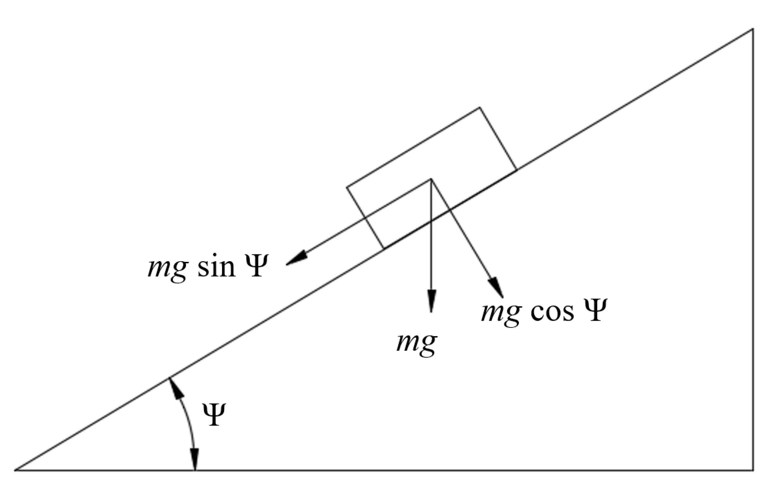
3.2. Inclined Plane Test

The inclined plane test has been used to determine soil–tool or soil–machine coefficients of static and rolling friction [29]. A schematic diagram of the setup for the inclined plane test is shown in Figure 10. A flat bed of the soil to be modelled is packed into a tray and held on a table with adjustable horizontal inclination. A block of tool material and ball bearings are separately placed on the flat bed, and the table is tilted to an angle Ψ at which the block just starts sliding or the ball just starts rolling down the inclination. The block is used for the determination of the soil–tool coefficient of static friction (µ_s), while the ball bearing is used in the determination of the soil–tool coefficient of rolling friction (µ_r). If the mass of the block is m_s, the mass of the ball is m_r, and the angles at which sliding and rolling occur are Ψ_s and Ψ_r, respectively, then the coefficients are calculated according to Equations (28) and (29) [29,97].

Soil–tool coefficient of static friction,

$${\mu }_s=\frac{m_{s}g\sin {\Psi }_s}{m_{s}g\cos {\Psi }_s}=\tan {\Psi }_s$$

(28)

Soil–tool coefficient of rolling friction,

$${\mu }_r=\frac{m_{r}g\sin {\Psi }_r}{m_{r}g\cos {\Psi }_r}=\tan {\Psi }_r$$

(29)

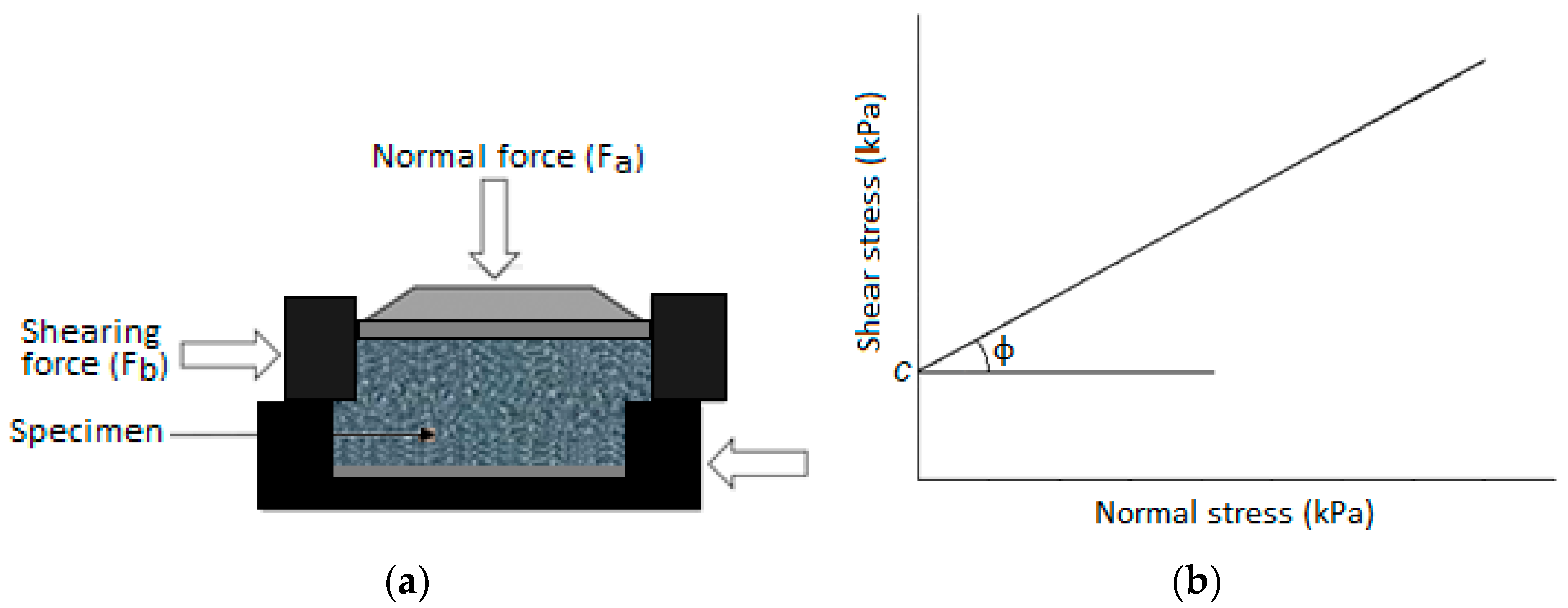
3.3. Direct Shear Test

The direct shear test is used to determine internal soil parameters namely, cohesion and internal friction angle (for soil-to-soil particle interactions). The modified shear test is used to determine the adhesion and external friction angle (for soil to tool or machine interface properties). These are typically used as direct DEM input parameters to support the calibration of other parameters. It has been used for cohesive and adhesive soils, as well as cohesionless soils [41,44,53].

This approach uses the normal and shear stresses acting on a column of granular materials’ cross-section. The experimental setup consists of two shear boxes, one placed on the other and filled with the granular material being modelled. One half is fixed while the other is made movable horizontally in one direction (Figure 11a). A specified normal force (F_a) is applied while an increasing horizontal (shearing) force (F_b) is applied to the movable half till a certain amount of displacement occurs [98]. At that point, the horizontal force would have reached a maximum value and remain constant or slightly increase or decrease afterward [30]. The experiment is repeated several times with different normal force values.

In the modified shear box test, the bottom half of the shear box is replaced with a material matching that of the tool or machine part. Normal force and shearing forces are applied the same way as described above. Corresponding normal and shear stresses are plotted as shown in Figure 11b. Given that the cohesive strength of the soil is c, the cross-sectional area of the shear box is A, and the internal friction angle is ϕ, the relationship between the normal force and the horizontal force is displayed in Equation (30).

F_b = cA + F_a tan ϕ

(30)

3.4. Triaxial Compression Test

This test can also determine the soil cohesive strength and internal friction angle and used to calibrate DEM input parameters for cohesive-frictional soils [52,72]. A triaxial compression test consists of loading an undisturbed cylindrical soil specimen insulated with an impermeable membrane and subjected to an adjustable confining pressure within a water chamber [18,99,100]. The specimen is then subjected to combined axial (σ₁) and radial (σ₃) stresses as indicated in Figure 12 until soil failure is achieved [98]. The radial stress (σ₃) is first applied around the specimen to a set level via the confining water pressure. An axial strain is then mechanically applied at a controlled rate which generates a corresponding additional deviator stress (q) logged over time and combining with σ₃ to form a resultant axial stress σ₁. The above steps are repeated several times under increasing radial stress. The plots of the deviator stress (q = σ₁ – σ₃) against axial strain identify each deviator stress value at failure and a simple process—for instance using the Mohr circle method—is then used to quantify soil cohesion and internal friction angle [101].

3.5. In Situ Approaches

Measurements of soil mechanical properties are most accurately done in the laboratory [103]. However, while laboratory methods can precisely measure soil properties, samples may not always be fully representative of field soil conditions due to sampling and handling limitations and time-related changes between sampling and testing. Hence, some researchers have used in situ approaches to measure soil properties for DEM calibration purposes. Kim et al. [44] used an on-site measurement system to determine soil mechanical properties such as shear modulus, Young’s modulus, and soil–tool static and rolling friction (Figure 13). On the other hand, Aikins et al. [41] used an on-site cone penetration test (Figure 14) to calibrate Young’s modulus of a Black Vertosol.

Asaf et al. [10] proposed grouser shear and sinkage or penetration tests using wedges of different wedge angles and a plate for calibrating DEM contact parameters. Jang et al. [82] also used a rectangular plate, while Ucgul et al. [38] and Ucgul et al. [29] used circular disc and cone penetration tests to calibrate model parameters. Cheng et al. [33] used a soil adhesion mass test to determine DEM input parameters of wet clay soil by employing the Plackett–Burman test and response surface methodology (RSM) to optimise input parameters.

4. Prediction of Soil Failure, Loosening, and Disturbance Parameters

4.1. Soil Failure and Loosening

Tamas et al. [30] and Barr et al. [21] have revealed the ability of DEM to predict soil rupture and crack propagation, which is an advantage over FEM. Some researchers have used velocity profiles [7,32] or displacement profiles [41,69,104] as soil loosening indicators. Others [21,30] used porosity (in PFC3D Particle Flow Code) or voidage (in EDEM 2.7^TM), respectively, to measure the degree of particles loosening in DEM. In the work of Tamas et al. [30], for instance, it was found that the DEM modelled soil porosity and soil-break-up resulting from loosening by sweeps increased with both increasing speed and rake angle, which agrees with experimental results.

Identifying particle movement or loosening is mainly used in defining the boundary between disturbed and undisturbed particles to simulate soil failure boundary or furrow profile. Barr et al. [21] argued that using velocity and displacement profiles is based on the assumption that particle movement results in only soil loosening, ignoring the fact that particle movement also occurs during a soil compaction process. The validity of this assumption is therefore limited to tools operating above their critical depth. Additionally, these approaches are open to subjective decisions since a threshold has to be arbitrarily defined to differentiate between the “so-called” loosened and unloosened particles. For example, Murray [69] had to describe loosened particles as having a displacement magnitude above 5 mm. Barr et al. [21] instead proposed and used a voidage grid (Figure 15) to define failure boundaries. A voidage grid was applied to the DEM particles after the tillage process was completed and the particles had settled, which reflects experimental practice. Voidage is similar to soil porosity as it measures the proportion of volume not occupied by particles. An empty space will have a voidage of 100%, while a completely filled space will have a voidage of 0%. With V_g being grid volume and V_p the total volume of particles whose centroids are located within the grid, voidage can be calculated according to Equation (31).

$$Voidage=\frac{V_g-V_p}{V_g}\times 100\%$$

(31)

Aikins et al. [41] used particle displacement (PD) analysis to determine the loosened furrow boundary in DEM. The displacement threshold was not set arbitrarily as was done by Murray [69]. Aikins et al. [41] defined the loosened furrow boundary based on two criteria:

• Minimum particle displacement caused directly by an opener occurs with particles just adjacent to the bottom part of the opener (for wide tines) or particles aligning the walls of the slot below critical depth (for narrow tines).
• To establish a sharp contrast between displaced and undisturbed particles, particle locations immediately after particle loosening (i.e., before the particle settle) has to be used.

Aikins et al. [41] traced the minimum particle displacement up the profile to produce a loosened furrow boundary as shown in Figure 16a. Figure 16a is a contour plot of the width and depth of the virtual soil bin profile against displacements (resultant) for each particle within the profile. In some studies [21,32], disturbed soil surface profile after tillage was determined using voidage grid binning and velocity profile. However, Aikins et al. [41] used the profile of the top surface of displaced DEM particles as the disturbed surface profile after the particles had settled because that gives more realistic results and is similar to what actually happens in field experiments. Wang et al. [74] employed another approach using the “clipping” module in EDEM simulation software to define the disturbed soil boundary (Figure 16b). The furrow profile was obtained by connecting the boundaries of the different layers of disturbed soil.

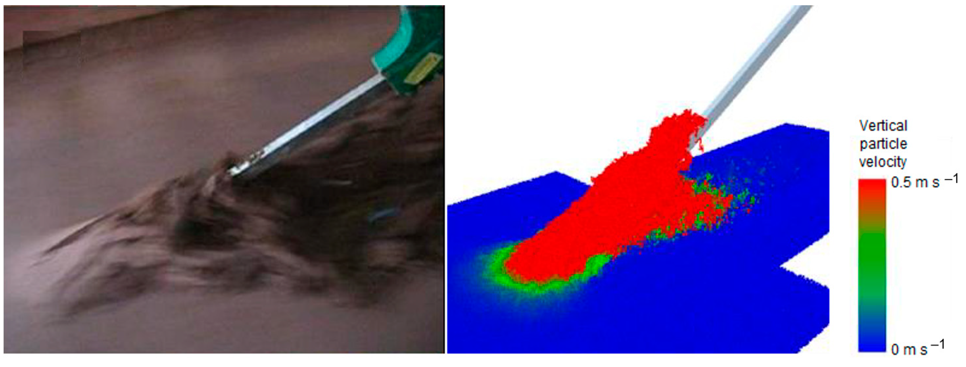
4.2. Soil Movement and Disturbance Parameters

From the loosened criteria described in the previous section, furrow profile, soil movement, and various soil disturbance parameters have been predicted or determined in DEM simulations with varying levels of relative error (RE) compared to experimental results. Such soil disturbance parameters include the lateral, forward, and upward movement of particles; furrow width at soil surface; loosened furrow cross-sectional area; furrow % backfill and dip area. Barr et al. [21] found an RE of 9% in loosened furrow cross-sectional area, 26% in furrow width, 14% in dip area, 0.8% in furrow backfill, 16% in ridge height, and 9% in lateral soil throw in a DEM prediction of soil disturbance parameters with narrow point openers operating in a sandy-loam soil. Barr and Fielke [105] closely predicted lateral soil throw and soil layer mixing using narrow tine openers with 35° and 90° rake angles and a bentleg opener (Figure 17). Using furrow openers with different rake angles and cutting edge cross-sections, Aikins et al. [41] closely predicted furrow profiles and similar patterns for surface profiles. The majority of DEM predictions of furrow cross-sectional area, furrow width, critical depth, and lateral soil throw had an RE of 1% to 20%. However, poor predictions were made for ridge height due to the use of large DEM particles (radius of 5 mm) [41].

Wang et al. [74] determined soil looseness, furrow width, soil disturbance coefficient, and soil disturbance area ratio with an RE from 3.24% to 41.64% for a winged subsoiler and 0.24% to 28.74% for a non-winged subsoiler. There was also a satisfactory agreement in “shape and magnitude” of lateral, forward, and upward displacement of different soil layers resulting from a sweep cultivator between experimental and DEM simulation results [62]. Using a disc with tilt angles from 0° to 20°, Murray [69] estimated an average absolute RE of about 10.53% for lateral soil throw. The DEM simulation also revealed, in agreement with the experimental result, that lateral soil throw increased with increasing tilt angle. For a hoe furrow opener, a RE of 14.8% was recorded.

Reduction in the forward movement of soil particles at greater depth has been predicted through DEM simulations [21,32,41]. Other researchers have previously described this phenomenon [9,106,107,108] through experimental work and analytical models in the concept of critical depth. Below the critical depth, soil movement changes from forward, sideways, and upward directions (generating a loosened crescent-shaped soil failure) to mainly forward and sideways, generating a compaction type failure in a horizontal plane. Barr et al. [21] and Aikins et al. [41] closely predicted the narrowing of furrow down the profile and critical depth with a 90° rake angle (Figure 15 and Figure 16a). Hang et al. [32] observed a reduction of the forward movement of particles in the inter-row zone between tines with increasing tine spacing in both DEM and experimental results. Greater inter-row zone soil movement with narrower tine spacing was attributed to more intensive interaction between tines. DEM can also simulate greater soil movement with wing attachment to tine cutting tools [31].

Greater soil upheaval observed with a low rake angle opener (35°) and increased lateral throw of soil (due to splashing effect) typically found with steeper (90°) rake angle openers have been successfully replicated with DEM [21]. However, Ucgul et al. [38] observed that the dynamic height of soil flow under sweep openers was under-predicted by 23% to 35% at speeds of 5 to 12.5 km/h and did not follow the observed shape using spherical particles of 10 mm radii. The prediction was improved by using smaller particles of radii 1.5 mm, which still underpredicted soil flow height by 15%. Using particles of smaller radii, however, considerably increased computation time. Lateral soil throw was also under predicted by about 32% and 9% with radii 10 and 1.5 mm, respectively.

Chen et al. [7] estimated a maximum of 3% RE in furrow cross-sectional area, up to 4% RE in disturbed width, from 14% to 26% more soil (by volume) heaped above the soil surface and 5% to 15% more emptied cross-section below the soil surface. Overall, a close agreement was observed between experimental and simulation results. Hang et al. [32] estimated less than 20% RE between DEM predicted and experimentally determined soil disturbance coefficient and soil looseness. Saunders et al. [76] reported significant underprediction and correlations between measured and predicted furrow area (r = 0.82) and maximum soil throw (r = 0.88) when optimizing the performance of a mouldboard skimmer in a sandy-loam soil. Several furrow parameters from bentleg openers operating in sandy-loam soil, including loosened cross-sectional area (RE = 14.9%), furrow dip area (RE = 14.4%), backfill (RE = 1.8%), ridge height (RE = 16.8%), and lateral soil throw (RE = 14.9%), were accurately predicted using the voidage grid bin approach [39]. Furthermore, Barr et al. [39] observed the same findings as those measured in soil bin investigations, with DEM simulations of bentleg openers also achieving 100% backfill and cancelling furrow spill over.

The DEM has also been used to simulate rotary tiller operations for design optimization. Zhang et al. [109] and Hirasawa et al. [110] closely predicted the height and pattern of soil surface undulations after rotary tillage in DEM. Soil movement pattern during rotary tillage and improving soil layer mixing with tillage depth and travel speed for a rotary tiller have also been closely predicted [36,109]. Cheng et al. [33] recorded an RE of 1.84% in mass of soil that adhered to rotary tiller blades.

5. Prediction of Tillage Forces

Most attention in the DEM simulation of soil cutting tools has been on predicting soil forces. Table 2 shows relative error (RE) values in draught and vertical force predictions with DEM, travel speed and operating depths for the stated tillage tools, soil types, and DEM contact models. Draught force cycles between peaks at incipient soil failure and troughs at the start of the reloading phase have been well captured in DEM simulations of sweeps by Tamas et al. [30]. In the same DEM study, draught was found to increase with greater speed and rake angle. Draught was predicted with 4% to 12% RE as speed was increased from 0.5 to 2.4 m s⁻¹ with a sweep tine. Bo et al. [31] observed a similar trend between draught force measured for four subsoilers in the soil bin and that obtained through DEM simulation. A winged subsoiler among the four had the highest draught force in both soil bin tests (up to 50% more) and simulations (up to 55% more). With all four subsoilers, DEM predicted draught force with relative errors below 4%.

Additionally, Wang et al. [74] showed that a winged subsoiler operating at a speed and depth of 3 km h⁻¹ and 300 mm, respectively, had an RE of 9.71%, whereas the non-winged subsoiler obtained an RE of 15.08% when the draught force was compared with the experimental result. Chen et al. [7] observed about 4–31% RE between the draught of experimental and DEM results. A good correlation was obtained between the measured and predicted draught forces (r = 0.95), whereas a more limited correlation was observed for vertical force (r = 0.71). With blunt (R90B) and chamfered (C2S) narrow openers with a 90° rake angle, a blunt opener with a 45° rake angle, and a bentleg opener, Aikins et al. [41] predicted draught force with REs of 20%, 22%, 31%, and 5%, respectively. Vertical force was also predicted with 8% and 20% relative error for R90B and C2S, respectively, but poorly for the two other openers.

DEM simulations with a mouldboard plough were also able to simulate the gradual entry of the mouldboard into the soil with a gradual draught increase. For the two soil conditions used in this study, 9% and 2.4% errors in cultivator tool draught were observed for a soft-wet soil and a hard-dry soil, respectively. DEM also closely predicted an increase in draught with increasing depth, with RE ranging from about 3% to 15% [56]. Kim et al. [44] observed that draught force increased with increasing depth with an overall average RE of 7.45%. Tong et al. [73] showed that, across four tillage depths, simulated draught and vertical forces were up to 10% smaller than those measured in the field.

In a DEM prediction of horizontal and vertical soil forces with DEM particles clumped to form different shapes (similar to that shown in Figure 7), Ono et al. [28] obtained the most accurate predictions with the three linearly overlapping spheres. The worst prediction was obtained with simple spherical particles. Ucgul et al. [38] observed a linear increase in draught force against sweep tine width measured experimentally and predicted using DEM with a maximum RE of 8%. Likewise, a non-linear increase in vertical force against width with a maximum RE of 13.7% was recorded. High correlations were recorded between measured and predicted draught forces (r = 0.978) and vertical forces (r = 0.971) with tool speeds from 5 to 12.5 km h⁻¹ and a depth of 70 mm. Prediction of the effect of rake angle on soil forces followed a similar trend (r values of 0.98 and 0.97) and had an RE of 11.6% and 15.2% for draught and vertical forces, respectively. Ucgul et al. [111] again obtained an accurate prediction of draught and vertical forces of a sweep tillage tool at varying speeds and geometry with r values ranging from 0.84 to 0.92. Murray [69] estimated an average RE of 1.86% for draught and 50.7% for vertical force with a flat single disc opener. For rotary tillers, Zhang et al. [109] reported a 12% RE in power consumption, while Du et al. [36] predicted increasing torque with tillage depth (150 to 180 mm) and travel speed (about 2 to 3 km h⁻¹).

6. Soils Modelled in DEM Simulations

Table 1 and Table 2 list soil types used in various tillage and furrow opener DEM simulations and their bulk densities, soil water contents, and cohesive strengths. It can be seen that most of the soils modelled with DEM are of sandy to sandy-loam textures. DEM modelling of highly cohesive soils is still relatively scarce in the literature. Bravo et al. [18] used DEM to model highly cohesive clay soil (Vertosol) with cohesive strength of up to about 125 kPa when the soil was highly compacted (bulk density of about 1400 kg m⁻³) and relatively dry (soil water content of about 18%). Aikins et al. [41] also modelled a Vertosol with cohesive strength of 46.4 kPa.

The properties and flow characteristics of sandy soils differ from those of clay soils, which show cohesive and adhesive properties in the presence of sufficient moisture. The successful modelling of a Vertosol and its interaction with tools in DEM by Bravo et al. [18] and Aikins et al. [41] revealed the ability of DEM to model cohesive soils. Although some authors [33,41,43,44,104,112,113] have recently modelled cohesive soils using DEM, more attention is needed in future research to cover the wide spectrum of agricultural soils.

7. Conclusions

Based on this review, the following conclusions can be drawn:

• Even though the Hertz–Mindlin contact model (HMCM) has been used in most DEM studies of tillage and furrow opening, it consistently fails to predict vertical soil force accurately. The Hysteretic Spring contact model (HSCM) can more accurately predict soil forces and particle movement.
• Angle of repose, inclined plane, direct shear, triaxial compression, and some in situ tests (grouser shear, plate sinkage, and cone penetration tests) have been used to measure and calibrate DEM input parameters. The angle of repose test has been used mainly for cohesionless soils due to the poor flowability of cohesive soils. However, using results from reproducible phases of the angle of repose experiment, successful calibrations for cohesive soils have been achieved.
• Unlike other numerical models, DEM is able to closely predict not only soil forces, but it is also capable of modelling soil failure mechanisms, soil loosening, and soil particle movement. Soil rupture and crack propagation, critical depth, three-dimensional particle movement within the soil profile and lateral particle movement on top of the soil have all been predicted in DEM.
• Using voidage or porosity grids to determine loosened furrow cross-sectional profiles has been found to be superior to using particle velocity and displacement profiles. However, some researchers have successfully used a particle displacement approach to determine accurate furrow profiles with a more objective criteria for defining loosened furrow boundary.
• Close predictions of draught and vertical forces (≤20%) have been obtained with DEM. These predictions can be improved by using smaller particles of a near-real shape. However, this must be balanced with computation time requirements.

Based on the review conducted, the following recommendations are made for future research:

• The Edinburgh elasto-plastic adhesion model (EEPA) has been successfully used to model consolidated or cohesive powders. This contact model is recommended to be studied more extensively for cohesive soils, although some researchers have used it.
• Due to pore water pressure within wet and soft soils, coupling DEM and CFD is likely to produce more accurate simulations. This idea can be explored in future research.
• A comprehensive analysis of soil disturbance parameters has been successfully done using voidage grids in EDEM^® DEM software. Replication of this approach in other DEM software is recommended.
• The criteria introduced by Aikins et al. [41] for defining particle displacement threshold for DEM furrow profile identification need further investigation with particles of smaller radii than the 5 mm used in the study. This approach can provide greater details on the three-dimensional soil translocation process.

References

1. Aybek, A.; Baser, E.; Arslan, S.; Ucgul, M. Determination of the effect of biodiesel use on power take-off performance characteristics of an agricultural tractor in a test laboratory. Turk. J. Agric. For. 2011, 35, 103–113. [Google Scholar] [CrossRef]
2. Kushwaha, R.L.; Zhang, Z.X. Evaluation of factors and current approaches related to the computerized design of tillage tools: A review. J. Terramechanics 1998, 35, 69–86. [Google Scholar] [CrossRef]
3. Aikins, K.A.; Barr, J.B.; Ucgul, M.; Jensen, T.A.; Antille, D.L.; Desbiolles, J.M.A. No-tillage furrow opener performance: A review of tool geometry, settings and interactions with soil and crop residue. Soil Res. 2020, 58, 603–621. [Google Scholar] [CrossRef]
4. McKyes, E. Soil Cutting and Tillage; Development in Agricultural Engineering Volume 7; Elsevier: Amsterdam, The Netherlands, 1985; Volume 7. [Google Scholar]
5. Godwin, R.J. A review of the effect of implement geometry on soil failure and implement forces. Soil Tillage Res. 2007, 97, 331–340. [Google Scholar] [CrossRef]
6. Shmulevich, I.; Asaf, Z.; Rubinstein, D. Interaction between soil and a wide cutting blade using the discrete element method. Soil Tillage Res. 2007, 97, 37–50. [Google Scholar] [CrossRef]
7. Chen, Y.; Munkholm, L.J.; Nyord, T. A discrete element model for soil-sweep interaction in three different soils. Soil Tillage Res. 2013, 126, 34–41. [Google Scholar] [CrossRef]
8. Hettiaratchi, D.R.P.; Reece, A.R. Symmetrical three-dimensional soil failure. J. Terramechanics 1967, 4, 45–67. [Google Scholar] [CrossRef]
9. Godwin, R.J.; Spoor, G. Soil failure with narrow tines. J. Agric. Eng. Res. 1977, 22, 213–228. [Google Scholar] [CrossRef]
10. Asaf, Z.; Rubinstein, D.; Shmulevich, I. Determination of discrete element model parameters required for soil tillage. Soil Tillage Res. 2007, 92, 227–242. [Google Scholar] [CrossRef]
11. Shmulevich, I. State of the art modeling of soil–tillage interaction using discrete element method. Soil Tillage Res. 2010, 111, 41–53. [Google Scholar] [CrossRef]
12. McKyes, E.; Ali, O.S. The cutting of soil by narrow blades. J. Terramechanics 1977, 14, 43–58. [Google Scholar] [CrossRef]
13. Godwin, R.J.; O’Dogherty, M.J. Integrated soil tillage force prediction models. J. Terramechanics 2007, 44, 3–14. [Google Scholar] [CrossRef]
14. Fielke, J.M. Finite element modelling of the interaction of the cutting edge of tillage implements with soil. J. Agric. Eng. Res. 1999, 74, 91–101. [Google Scholar] [CrossRef]
15. Karmakar, S.; Ashrafizadeh, S.R.; Kushwaha, R.L. Experimental validation of computational fluid dynamics modeling for narrow tillage tool draft. J. Terramechanics 2009, 46, 277–283. [Google Scholar] [CrossRef]
16. Cundall, P.A.; Strack, O.D.L. A discrete numerical model for granular assemblies. Geotechnique 1979, 29, 47–65. [Google Scholar] [CrossRef]
17. Franco, Y.; Rubinstein, D.; Shmulevich, I. Prediction of soil-bulldozer blade interaction using discrete element method. Trans. ASABE 2007, 50, 345–353. [Google Scholar] [CrossRef]
18. Bravo, E.L.; Tijskens, E.; Suarez, M.H.; Cueto, O.G.; Ramon, H. Prediction model for non-inversion soil tillage implemented on discrete element method. Comput. Electron. Agric. 2014, 106, 120–127. [Google Scholar] [CrossRef]
19. Markauskas, D.; Ramírez-Gómez, Á.; Kačianauskas, R.; Zdancevičius, E. Maize grain shape approaches for DEM modelling. Comput. Electron. Agric. 2015, 118, 247–258. [Google Scholar] [CrossRef]
20. Coetzee, C.J. Review: Calibration of the discrete element method. Powder Technol. 2017, 310, 104–142. [Google Scholar] [CrossRef]
21. Barr, J.B.; Ucgul, M.; Desbiolles, J.M.A.; Fielke, J.M. Simulating the effect of rake angle on narrow opener performance with the discrete element method. Biosyst. Eng. 2018, 171, 1–15. [Google Scholar] [CrossRef]
22. Peng, B. Discrete Element Method (DEM) Contact Models Applied to Pavement Simulation. Unpublished. Master’s Thesis, Virginia Polytechnic Institute and State University, Blacksburg, Virginia, 2014. [Google Scholar]
23. Luding, S. Introduction to discrete element methods: Basics of contact force models and how to perform the micro-macro transition to continuum theory. Eur. J. Environ. Civ. Eng. 2008, 12, 785–826. [Google Scholar] [CrossRef]
24. Horabik, J.; Molenda, M. Parameters and contact models for DEM simulations of agricultural granular materials. Biosyst. Eng. 2016, 147, 206–229. [Google Scholar] [CrossRef]
25. Tamás, K.; Bernon, L. Role of particle shape and plant roots in the discrete element model of soil–sweep interaction. Biosyst. Eng. 2021, 211, 77–96. [Google Scholar] [CrossRef]
26. Ucgul, M. Simulation of Sweep Tillage Using Discrete Element Modelling. Unpublished. Ph.D. Thesis, University of South Australia, Adelaide, Australia, 2014. [Google Scholar]
27. Tanaka, H.; Momozu, M.; Oida, A.; Yamazaki, M. Simulation of soil deformation and resistance at bar penetration by the Distinct Element Method. J. Terramechanics 2000, 37, 41–56. [Google Scholar] [CrossRef]
28. Ono, I.; Nakashima, H.; Shimizu, H.; Miyasaka, J.; Ohdoi, K. Investigation of elemental shape for 3D DEM modeling of interaction between soil and a narrow cutting tool. J. Terramechanics 2013, 50, 265–276. [Google Scholar] [CrossRef] [Green Version]
29. Ucgul, M.; Fielke, J.M.; Saunders, C. Three-dimensional discrete element modelling of tillage: Determination of a suitable contact model and parameters for a cohesionless soil. Biosyst. Eng. 2014, 121, 105–117. [Google Scholar] [CrossRef]
30. Tamas, K.; Jori, I.J.; Mouazen, A.M. Modelling soil-sweep interaction with discrete element method. Soil Tillage Res. 2013, 134, 223–231. [Google Scholar] [CrossRef] [Green Version]
31. Bo, L.; Rui, X.; Liu, F.Y.; Jun, C.; Han, W.T.; Bing, H. Determination of the draft force for different subsoiler points using discrete element method. Int. J. Agr. Biol. Eng. 2016, 9, 81–87. [Google Scholar] [CrossRef]
32. Hang, C.; Gao, X.; Yuan, M.; Huang, Y.; Zhu, R. Discrete element simulations and experiments of soil disturbance as affected by the tine spacing of subsoiler. Biosyst. Eng. 2018, 168, 73–82. [Google Scholar] [CrossRef]
33. Cheng, J.; Zheng, K.; Xia, J.; Liu, G.; Jiang, L.; Li, D. Analysis of adhesion between wet clay soil and rotary tillage part in paddy field based on discrete element method. Processes 2021, 9, 845. [Google Scholar] [CrossRef]
34. Yang, Y.; Wen, B.; Ding, L.; Li, L.; Chen, X.; Li, J. Soil Particle Modeling and Parameter Calibration for Use with Discrete Element Method. Trans. ASABE 2021, 64, 2011–2023. [Google Scholar] [CrossRef]
35. Hoseinian, S.H.; Hemmat, A.; Esehaghbeygi, A.; Shahgoli, G.; Baghbanan, A. Development of a dual sideway-share subsurface tillage implement: Part 1. Modeling tool interaction with soil using DEM. Soil Tillage Res. 2022, 215, 105201. [Google Scholar] [CrossRef]
36. Du, J.; Heng, Y.; Zheng, K.; Luo, C.; Zhu, Y.; Zhang, J.; Xia, J. Investigation of the burial and mixing performance of a rotary tiller using discrete element method. Soil Tillage Res. 2022, 220, 105349. [Google Scholar] [CrossRef]
37. Zhai, S.; Shi, Y.; Zhou, J.; Liu, J.; Huang, D.; Zou, A.; Jiang, P. Simulation optimization and experimental study of the working performance of a vertical rotary tiller based on the discrete element method. Actuators 2022, 11, 324. [Google Scholar] [CrossRef]
38. Ucgul, M.; Fielke, J.M.; Saunders, C. 3D DEM tillage simulation: Validation of a hysteretic spring (plastic) contact model for a sweep tool operating in a cohesionless soil. Soil Tillage Res. 2014, 144, 220–227. [Google Scholar] [CrossRef]
39. Barr, J.; Desbiolles, J.; Ucgul, M.; Fielke, J.M. Bentleg furrow opener performance analysis using the discrete element method. Biosyst. Eng. 2020, 189, 99–115. [Google Scholar] [CrossRef]
40. Makange, N.R.; Ji, C.; Torotwa, I. Prediction of cutting forces and soil behavior with discrete element simulation. Comput. Electron. Agric. 2020, 179, 105848. [Google Scholar] [CrossRef]
41. Aikins, K.A.; Ucgul, M.; Barr, J.B.; Jensen, T.A.; Antille, D.L.; Desbiolles, J.M.A. Determination of discrete element model parameters for a cohesive soil and validation through narrow point opener performance analysis. Soil Tillage Res. 2021, 213, 105123. [Google Scholar] [CrossRef]
42. Awuah, E.; Zhou, J.; Liang, Z.; Aikins, K.A.; Gbenontin, B.V.; Mecha, P.; Makange, N.R. Parametric analysis and numerical optimisation of Jerusalem artichoke vibrating digging shovel using discrete element method. Soil Tillage Res. 2022, 219, 105344. [Google Scholar] [CrossRef]
43. Wang, X.; Zhang, Q.; Huang, Y.; Ji, J. An efficient method for determining DEM parameters of a loose cohesive soil modelled using hysteretic spring and linear cohesion contact models. Biosyst. Eng. 2022, 215, 283–294. [Google Scholar] [CrossRef]
44. Kim, Y.-S.; Siddique, M.A.A.; Kim, W.-S.; Kim, Y.-J.; Lee, S.-D.; Lee, D.-K.; Hwang, S.-J.; Nam, J.-S.; Park, S.-U.; Lim, R.-G. DEM simulation for draft force prediction of moldboard plow according to the tillage depth in cohesive soil. Comput. Electron. Agric. 2021, 189, 106368. [Google Scholar] [CrossRef]
45. Wu, Z.; Wang, X.; Liu, D.; Xie, F.; Ashwehmbom, L.G.; Zhang, Z.; Tang, Q. Calibration of discrete element parameters and experimental verification for modelling subsurface soils. Biosyst. Eng. 2021, 212, 215–227. [Google Scholar] [CrossRef]
46. Zhao, Z.; Li, H.; Liu, J.; Yang, S.X. Control method of seedbed compactness based on fragment soil compaction dynamic characteristics. Soil Tillage Res. 2020, 198, 104551. [Google Scholar] [CrossRef]
47. Sun, J.; Chen, H.; Wang, Z.; Ou, Z.; Yang, Z.; Liu, Z.; Duan, J. Study on plowing performance of EDEM low-resistance animal bionic device based on red soil. Soil Tillage Res. 2020, 196, 104336. [Google Scholar] [CrossRef]
48. Dai, F.; Song, X.; Zhao, W.; Shi, R.; Zhang, F.; Zhang, X. Mechanism analysis and performance improvement of mechanized ridge forming of whole plastic film mulched double ridges. Int. J. Agric. Biol. Eng. 2020, 13, 107–116. [Google Scholar] [CrossRef]
49. Barr, J. Optimising bentleg opener geometry for higher speed no-till seeding. Unpublished Ph.D. Thesis, University of South Australia, Mawson Lakes, South Australia, Australia, 2018. [Google Scholar]
50. EDEM. EDEM 2020 Documentation; DEM Solutions: Edinburgh, UK, 2020. [Google Scholar]
51. Tamás, K.; Kovács, Á.; Jóri, I.J. The evaluation of the parallel bond’s properties in DEM modeling of soils. Period. Polytech. Mech. Eng. 2016, 60, 21–31. [Google Scholar] [CrossRef] [Green Version]
52. Obermayr, M.; Vrettos, C.; Eberhard, P. A discrete element model for cohesive soil. In Proceedings of the III International Conference on Particle-Based Methods—Fundamentals and Applications, Stuttgart, Germany, 18–20 September 2013; pp. 783–794. [Google Scholar]
53. Ucgul, M.; Fielke, J.M.; Saunders, C. Three-dimensional discrete element modelling (DEM) of tillage: Accounting for soil cohesion and adhesion. Biosyst. Eng. 2015, 129, 298–306. [Google Scholar] [CrossRef]
54. Potyondy, D.O.; Cundall, P.A. A bonded-particle model for rock. Int. J. Rock Mech. Min. Sci. 2004, 41, 1329–1364. [Google Scholar] [CrossRef]
55. Tekeste, M.Z.; Balvanz, L.R.; Hatfield, J.L.; Ghorbani, S. Discrete element modeling of cultivator sweep-to-soil interaction: Worn and hardened edges effects on soil-tool forces and soil flow. J. Terramechanics 2019, 82, 1–11. [Google Scholar] [CrossRef] [Green Version]
56. Li, B.; Liu, F.Y.; Mu, J.Y.; Chen, J.; Han, W.T. Distinct element method analysis and field experiment of soil resistance applied on the subsoiler. Int. J. Agric. Biol. Eng. 2014, 7, 54–59. [Google Scholar] [CrossRef]
57. Mak, J.; Chen, Y.; Sadek, M.A. Determining parameters of a discrete element model for soil–tool interaction. Soil Tillage Res. 2012, 118, 117–122. [Google Scholar] [CrossRef]
58. Sadek, M.A.; Chen, Y.; Liu, J. Simulating shear behavior of a sandy soil under different soil conditions. J. Terramechanics 2011, 48, 451–458. [Google Scholar] [CrossRef]
59. Van der Linde, J. Discrete Element Modeling of a Vibratory Subsoiler. Unpublished MSc. Thesis, University of Stellenbosch, Matieland, South Africa, 2007. [Google Scholar]
60. Kotrocz, K.; Mouazen, A.M.; Kerenyi, G. Numerical simulation of soil-cone penetrometer interaction using discrete element method. Comput. Electron. Agric. 2016, 125, 63–73. [Google Scholar] [CrossRef] [Green Version]
61. Mak, J.; Chen, Y. Simulation of draft forces of a sweep in a loamy sand soil using the discrete element method. Can.Biosyst.Eng. 2014, 56, 2.1–2.7. [Google Scholar] [CrossRef]
62. Milkevych, V.; Munkholm, L.J.; Chen, Y.; Nyord, T. Modelling approach for soil displacement in tillage using discrete element method. Soil Tillage Res. 2018, 183, 60–71. [Google Scholar] [CrossRef]
63. Sadek, M.; Chen, Y. Feasibility of using PFC3D to simulate soil flow resulting from a simple soil-engaging tool. Trans. ASABE 2015, 58, 987–996. [Google Scholar] [CrossRef]
64. Zeng, Z.; Chen, Y. Simulation of soil-micropenetrometer interaction using the discrete element method (DEM). Trans. ASABE 2016, 59, 1157–1163. [Google Scholar] [CrossRef]
65. Zeng, Z.; Chen, Y.; Zhang, X. Modelling the interaction of a deep tillage tool with heterogeneous soil. Comput. Electron. Agric. 2017, 143, 130–138. [Google Scholar] [CrossRef]
66. Zeng, Z.W.; Chen, Y. Simulation of straw movement by discrete element modelling of straw-sweep-soil interaction. Biosyst. Eng. 2019, 180, 25–35. [Google Scholar] [CrossRef]
67. Zhang, R.; Li, J. Simulation on mechanical behavior of cohesive soil by Distinct Element Method. J. Terramechanics 2006, 43, 303–316. [Google Scholar] [CrossRef]
68. Gupta, V.; Sun, X.; Xu, W.; Sarv, H.; Farzan, H. A discrete element method-based approach to predict the breakage of coal. Adv. Powder Technol. 2017, 28, 2665–2677. [Google Scholar] [CrossRef]
69. Murray, S. Modelling of Soil-Tool Interactions Using the Discrete Element Method. Unpublished MSc. Thesis, University of Manitoba, Winnipeg, MB, Canada, 2016. [Google Scholar]
70. Li, B.; Chen, Y.; Chen, J. Modeling of soil-claw interaction using the discrete element method (DEM). Soil Tillage Res. 2016, 158, 177–185. [Google Scholar] [CrossRef]
71. Johnson, K.L.; Kendall, K.; Roberts, A.D. Surface energy and the contact of elastic solids. Proc. R. Soc. Lond. Ser. A Math. Phys. Sci. 1971, 324, 301–313. [Google Scholar]
72. Obermayr, M.; Vrettos, C.; Eberhard, P.; Dauwel, T. A discrete element model and its experimental validation for the prediction of draft forces in cohesive soil. J. Terramechanics 2014, 53, 93–104. [Google Scholar] [CrossRef]
73. Tong, J.; Jiang, X.-H.; Wang, Y.-M.; Ma, Y.-H.; Li, J.-W.; Sun, J.-Y. Tillage force and disturbance characteristics of different geometric-shaped subsoilers via DEM. Adv. Manuf. 2020, 8, 392–404. [Google Scholar] [CrossRef]
74. Wang, X.; Li, P.; He, J.; Wei, W.; Huang, Y. Discrete element simulations and experiments of soil-winged subsoiler interaction. Int. J. Agric. Biol. Eng. 2021, 14, 50–62. [Google Scholar] [CrossRef]
75. Sadek, M.A.; Chen, Y.; Zeng, Z. Draft force prediction for a high-speed disc implement using discrete element modelling. Biosyst. Eng. 2021, 202, 133–141. [Google Scholar] [CrossRef]
76. Saunders, C.; Ucgul, M.; Godwin, R.J. Discrete element method (DEM) simulation to improve performance of a mouldboard skimmer. Soil Tillage Res. 2021, 205, 104764. [Google Scholar] [CrossRef]
77. Ma, S.; Niu, C.; Yan, C.; Tan, H.; Xu, L. Discrete element method optimisation of a scraper to remove soil from ridges formed to cold-proof grapevines. Biosyst. Eng. 2021, 210, 156–170. [Google Scholar] [CrossRef]
78. Morrissey, J.P.; Thakur, S.C.; Ooi, J.Y. EDEM Contact Model: Adhesive Elasto-Plastic Model; School of Engineering, University of Edinburgh: Edinburgh, UK, 2014. [Google Scholar]
79. Thakur, S.C.; Morrissey, J.P.; Sun, J.; Chen, J.F.; Ooi, J.Y. Micromechanical analysis of cohesive granular materials using the discrete element method with an adhesive elasto-plastic contact model. Granul Matter 2014, 16, 383–400. [Google Scholar] [CrossRef]
80. Schoeneberger, P.J.; Wysocki, D.A.; Benham, E.C.; Soil Survey Staff. Field Book for Describing and Sampling Soils; version 3.0; Natural Resources Conservation Service, National Soil Survey Center: Lincoln, NE, USA, 2012.
81. Morrissey, J.P. Discrete Element Modelling of Iron Ore Pellets to Include the Effects of Moisture and Fines. Unpublished Ph.D. Thesis, University of Edinburgh, Edinburgh, UK, 2013. [Google Scholar]
82. Jang, G.; Lee, S.; Lee, K.J. Discrete element method for the characterization of soil properties in Plate-Sinkage tests. J. Mech. Sci. Technol. 2016, 30, 2743–2751. [Google Scholar] [CrossRef]
83. Mousaviraad, M.; Tekeste, M.; Rosentrater, K. Discrete element method (DEM) simulation of corn grain flow in commercial screw auger. In Proceedings of the 2016 American Society of Agricultural and Biological Engineers Annual International Meeting, Orlando, FL, USA, 17–20 July 2016. [Google Scholar]
84. Coetzee, C.J. Calibration of the discrete element method and the effect of particle shape. Powder Technol. 2016, 297, 50–70. [Google Scholar] [CrossRef]
85. Smith, W.; Melanz, D.; Senatore, C.; Iagnemma, K.; Peng, H.E. Comparison of discrete element method and traditional modeling methods for steady-state wheel-terrain interaction of small vehicles. J. Terramechanics 2014, 56, 61–75. [Google Scholar] [CrossRef]
86. Adajar, J.B.; Alfaro, M.; Chen, Y.; Zeng, Z. Calibration of discrete element parameters of crop residues and their interfaces with soil. Comput. Electron. Agric. 2021, 188, 106349. [Google Scholar] [CrossRef]
87. Hernández-Vielma, C.; Estay, D.; Cruchaga, M. Response surface methodology calibration for DEM study of the impact of a spherical bit on a rock. Simul. Model. Pract. Theory 2022, 116, 102466. [Google Scholar] [CrossRef]
88. Mudarisov, S.; Farkhutdinov, I.; Khamaletdinov, R.; Khasanov, E.; Mukhametdinov, A. Evaluation of the significance of the contact model particle parameters in the modelling of wet soils by the discrete element method. Soil Tillage Res. 2022, 215, 105228. [Google Scholar] [CrossRef]
89. Qiu, Y.; Guo, Z.; Jin, X.; Zhang, P.; Si, S.; Guo, F. Calibration and Verification Test of Cinnamon Soil Simulation Parameters Based on Discrete Element Method. Agriculture 2022, 12, 1082. [Google Scholar] [CrossRef]
90. Zeng, F.; Li, X.; Zhang, Y.; Zhao, Z.; Cheng, C. Using the discrete element method to analyze and calibrate a model for the interaction between a planting device and soil particles. INMATEH Agric. Eng. 2021, 413–424. [Google Scholar] [CrossRef]
91. Zhu, J.; Zou, M.; Liu, Y.; Gao, K.; Su, B.; Qi, Y. Measurement and calibration of DEM parameters of lunar soil simulant. Acta Astronaut. 2022, 191, 169–177. [Google Scholar] [CrossRef]
92. Al-Hashemi, H.M.B.; Al-Amoudi, O.S.B. A review on the angle of repose of granular materials. Powder Technol. 2018, 330, 397–417. [Google Scholar] [CrossRef]
93. Qi, L.; Chen, Y.; Sadek, M. Simulations of soil flow properties using the discrete element method (DEM). Comput. Electron. Agric. 2019, 157, 254–260. [Google Scholar] [CrossRef]
94. Li, P.; Ucgul, M.; Lee, S.H.; Saunders, C. A new approach for the automatic measurement of the angle of repose of granular materials with maximal least square using digital image processing. Comput. Electron. Agric. 2020, 172, 105356. [Google Scholar] [CrossRef]
95. Rackl, M.; Hanley, K.J. A methodical calibration procedure for discrete element models. Powder Technol. 2017, 307, 73–83. [Google Scholar] [CrossRef] [Green Version]
96. Roessler, T.; Katterfeld, A. DEM parameter calibration of cohesive bulk materials using a simple angle of repose test. Particuology 2019, 45, 105–115. [Google Scholar] [CrossRef]
97. Aikins, K.A. Performance of Bentleg Opener for High Speed No-Tillage Sowing in Cohesive Soil. Unpublished. Ph.D. Thesis, University of Southern Queensland, Toowoomba, QLD, Australia, 2020. [Google Scholar]
98. Syed, Z.; Tekeste, M.; White, D. A coupled sliding and rolling friction model for DEM calibration. J. Terramechanics 2017, 72, 9–20. [Google Scholar] [CrossRef]
99. Rees, S. Introduction to Triaxial Testing: Part 1; GDS Instruments: Hampshire, UK, 2013. [Google Scholar]
100. Wang, Y.; Guo, P.; Dai, F.; Li, X.; Zhao, Y.; Liu, Y. Behavior and Modeling of Fiber-Reinforced Clay under Triaxial Compression by Combining the Superposition Method with the Energy-Based Homogenization Technique. Int. J. Geomech. 2018, 18, 04018172. [Google Scholar] [CrossRef]
101. Bardet, J.P. Experimental Soil Mechanics; Prentice-Hall: Upper Saddle River, NJ, USA, 1997. [Google Scholar]
102. Ahlinhan, M.F.; Houehanou, E.; Koube, M.B.; Doko, V.; Alaye, Q.; Sungura, N.; Adjovi, E. Experiments and 3D DEM of Triaxial Compression Tests under Special Consideration of Particle Stiffness. Geomaterials 2018, 8, 39–62. [Google Scholar] [CrossRef] [Green Version]
103. Das, B.M. Advanced Soil Mechanics, 5th ed.; CRC Press: Boca Raton, FL, USA, 2019. [Google Scholar] [CrossRef]
104. Aikins, K.A.; Barr, J.B.; Antille, D.L.; Ucgul, M.; Jensen, T.A.; Desbiolles, J.M.A. Analysis of effect of bentleg opener geometry on performance in cohesive soil using the discrete element method. Biosyst. Eng. 2021, 209, 106–124. [Google Scholar] [CrossRef]
105. Barr, J.; Fielke, J. Discrete element modelling of narrow point openers to improve soil disturbance characteristics of no-till seeding systems. In Proceedings of the ASABE Annual International Meeting, Orlando, FL, USA, 17–20 July 2016. [Google Scholar]
106. Spoor, G.; Godwin, R.J. An experimental investigation into the deep loosening of soil by rigid tines. J. Agric. Eng. Res. 1978, 23, 243–258. [Google Scholar] [CrossRef]
107. Spoor, G.; Fry, R.K. Soil disturbance generated by deep-working low rake angle narrow tines. J. Agric. Eng. Res. 1983, 28, 217–234. [Google Scholar] [CrossRef]
108. Conte, O.; Levien, R.; Debiasi, H.; Sturmer, S.L.K.; Mazurana, M.; Muller, J. Soil disturbance index as an indicator of seed drill efficiency in no-tillage agrosystems. Soil Tillage Res. 2011, 114, 37–42. [Google Scholar] [CrossRef]
109. Zhang, X.; Zhang, L.; Hu, X.; Wang, H.; Shi, X.; Ma, X. Simulation of soil cutting and power consumption optimization of a typical rotary tillage soil blade. Appl. Sci. 2022, 12, 8177. [Google Scholar] [CrossRef]
110. Hirasawa, K.; Kataoka, T.; Kubo, T. Prediction and evaluation for leveling performance in rotary tiller. In Proceedings of the 4th IFAC Conference on Modelling and Control in Agriculture, Espoo, FL, USA, 27–30 August 2013; pp. 315–320. [Google Scholar]
111. Ucgul, M.; Fielke, J.M.; Saunders, C. Defining the effect of sweep tillage tool cutting edge geometry on tillage forces using 3D discrete element modelling. Inf. Process. 2015, 2, 130–141. [Google Scholar] [CrossRef] [Green Version]
112. Aikins, K.A.; Antille, D.L.; Ucgul, M.; Jensen, T.A.; Barr, J.B.; Desbiolles, J.M.A. Analysis of effects of operating speed and depth on bentleg opener performance in cohesive soil using the discrete element method. Comput. Electron. Agric. 2021, 187, 106236. [Google Scholar] [CrossRef]
113. Karkala, S.; Davis, N.; Wassgren, C.; Shi, Y.; Liu, X.; Riemann, C.; Yacobian, G.; Ramachandran, R. Calibration of Discrete-Element-Method Parameters for Cohesive Materials Using Dynamic-Yield-Strength and Shear-Cell Experiments. Processes 2019, 7, 278. [Google Scholar] [CrossRef] [Green Version]
Figure 1. Discrete element method simulation of a narrow tine furrow opener operating in a moist sandy-loam soil. Modified from Barr et al. [21].
Agriculture 13 00541 g001
Figure 2. A schematic diagram of the normal (left) and tangential (right) components of the linear spring contact model.
Agriculture 13 00541 g002
Figure 3. Hysteretic spring force –displacement relationship used in the Hertz–Mindlin contact model (HMCM). Redrawn from Ucgul et al. [29]. The dashed line contrasts the basic linear elastic model relationship.
Agriculture 13 00541 g003
Figure 4. Hysteretic spring force-displacement relationship used in the hysteretic spring contact model (HSCM). Redrawn from Ucgul et al. [29].
Agriculture 13 00541 g004
Figure 5. The parallel bond model depicted as cylindrical bond between two particles.
Agriculture 13 00541 g005
Figure 6. Edinburgh elasto-plastic adhesion model (EEPA) normal contact force-displacement relationship (a) linear and (b) non-linear [50].
Agriculture 13 00541 g006
Figure 7. Different associations of spherical DEM particles used to more realistically account for the effects of soil particle shape on bulk behaviour.
Agriculture 13 00541 g007
Figure 8. Angle of repose test setup used by (a) Ucgul et al. [29] for a cohesionless soil, (b) Mousaviraad et al. [83] for maize, and (c) Roessler and Katterfeld [96] for a cohesive soil.
Agriculture 13 00541 g008
Figure 9. Repeatable dome-like soil pile obtained in the angle of repose test for a loose cohesive soil by Aikins et al. [41]: (a) laboratory experiment and (b) optimized DEM simulation.
Agriculture 13 00541 g009
Figure 10. Schematic diagram of inclined plane test setup with a block [97] for static friction coefficient. A ball can be used as well for rolling friction coefficient as found in Ucgul et al. [29].
Agriculture 13 00541 g010
Figure 11. (a) Direct shear box schematic, and (b) normal and shear stress expected relationship.
Agriculture 13 00541 g011
Figure 12. Specimen stress state in a triaxial compression test: retrieved from (a) Rees [99] and (b) Ahlinhan et al. [102].
Agriculture 13 00541 g012
Figure 13. Instruments for in situ measurements of soil mechanical properties: (a) sampled undisturbed soil specimen, (b) soil–metal static friction, (c) soil–metal rolling friction, (d) direct shear test, (e) shear modulus, and (f) Young’s modulus. Retrieved from Kim et al. [44].
Agriculture 13 00541 g013
Figure 14. (a) Motorised cone penetrometer for in situ measurements, and (b) DEM cone penetration simulation used by Aikins et al. [41].
Agriculture 13 00541 g014
Figure 15. Furrow profiles created using voidage grid bins in EDEM 2.7TM. Adapted from Barr [49].
Agriculture 13 00541 g015
Figure 16. Definitions of furrow boundary used by (a) Aikins et al. [41] and (b) Wang et al. [74].
Agriculture 13 00541 g016
Figure 17. Comparison of furrow profiles for 16 mm wide narrow openers at different rake angles (35°, 53°, 72°, and 90°) obtained from soil bin experiment and DEM simulations. Retrieved and modified from Barr [49].
Agriculture 13 00541 g017