Article

Using Artificial Intelligence Algorithms to Estimate and Short-Term Forecast the Daily Reference Evapotranspiration with Limited Meteorological Variables

1
Department of Agronomy, National Chung Hsing University, Taichung 40227, Taiwan
2
Taiwan Seed Improvement and Propagation Station, Taichung 426017, Taiwan
3
Smart Sustainable New Agriculture Research Center (SMARTer), Taichung 40227, Taiwan
*
Author to whom correspondence should be addressed.
These authors contributed equally to this work.
Submission received: 15 February 2024 / Revised: 20 March 2024 / Accepted: 20 March 2024 / Published: 22 March 2024
(This article belongs to the Special Issue Application of Machine Learning and Data Analysis in Agriculture)

Abstract

:
The reference evapotranspiration (ET0) information is crucial for irrigation planning and water resource management. While the Penman-Monteith (PM) equation is widely recognized for ET0 calculation, its reliance on numerous meteorological parameters constrains its practical application. This study used 28 years of meteorological data from 18 stations in four geographic regions of Taiwan to evaluate the effectiveness of an artificial intelligence (AI) model for estimating PM-calculated ET0 using limited meteorological variables as input and compared it with traditional methods. The AI models were also employed for short-term ET0 forecasting with limited meteorological variables. The findings suggested that AI models performed better than their counterpart methods for ET0 estimation. The artificial neural network using temperature, solar radiation, and relative humidity as input variables performed best, with the correlation coefficient (r) ranging from 0.992 to 0.998, mean absolute error (MAE) ranging from 0.07 to 0.16 mm/day, and root mean square error (RMSE) ranging from 0.12 to 0.25 mm/day. For short-term ET0 forecasting, the long short-term memory model using temperature, solar radiation, and relative humidity as input variables was the best structure to forecast four-day-ahead ET0, with the r ranging from 0.608 to 0.756, MAE ranging from 1.05 to 1.28 mm/day, and RMSE ranging from 1.35 to 1.62 mm/day. The percentage error of this structure was within ± 5% for most meteorological stations over the one-year test period, underscoring the potential of the proposed models to deliver daily ET0 forecasts with acceptable accuracy. Finally, the proposed estimating and forecasting models were developed in regional and variable-limited scenarios, making them highly advantageous for practical applications.

1. Introduction

With the escalation of the global population and the concomitant rise in water demand, effectively managing limited water resources while sustaining productivity has become an important issue in agriculture today [1]. Consequently, assessing crop water demand has become crucial to achieving a precise allocation of water resources [1,2]. Crop water demand can be obtained from the product of reference evapotranspiration (ET0) and crop-specific coefficients [2,3]. Moreover, ET0 can serve to characterize local climatic conditions or aid in calculating drought indices for drought monitoring [4,5,6]. Therefore, an accurate estimation of ET0 is essential for irrigation planning and water resource management.
ET0 is defined as the evapotranspiration of a hypothetical crop with a plant height of 0.12 m, a fixed surface resistance of 70 s/m, and an albedo of 0.23 [7]. Although ET0 can be measured by a lysimeter, the use of this instrument in practical applications is typically constrained by cost and operational intricacies, making it more suitable for research purposes [8,9]. Conversely, the approach of using the meteorological data recorded by weather stations to establish ET0 equations through mathematical and physical theories is a more practical avenue for application [10].
Among the existing ET0 equations, the Penman-Monteith (PM) equation stands out as the most renowned [11,12]. The PM equation is deduced based on energy balance and water vapor diffusion, and it also considers crop canopy resistance and aerodynamic resistance. Since the laws of physics do not change from location to location, the physics-based PM equation is sufficient as a basis for estimating ET0 globally when high-quality meteorological data can be obtained [13]. Therefore, the PM equation was recommended as a standard method for estimating ET0 in the FAO-56 report of the Food and Agriculture Organization (FAO) of the United Nations in 1998. Subsequent sensitivity analyses and regional assessments have confirmed the applicability of the PM equation across diverse environments [10,13]. However, the application of the PM equation requires many meteorological parameters including, solar radiation (Rs), mean air temperature (T), mean relative humidity (RH), and mean wind speed at 2 m above ground (u2). The construction and maintenance of corresponding sensors can be expensive. In addition, it is difficult to collect reliable meteorological data in some regions, or some parameters cannot be achieved [14]. Therefore, developing methods that could accurately estimate ET0 using a subset of meteorological variables had value from either a cost or practical perspective.
Three strategies have been developed to address the absence of requisite parameters for the PM equation, including using PM-alternative equations, estimating the lacking meteorological variable(s), and estimating the ET0 based on artificial intelligence (AI) algorithms. The FAO recommends initially estimating the lacking meteorological variable and then plugging the estimate into the PM equation [13], an approach known as the reduced-set PM (RPM) [15,16]. There are also PM-alternative equations such as Hargreaves-Samani (HS), Makkink, and Turc equations that require fewer meteorological variables and are easier to compute than the PM equation. However, the performance of these equations varies from location to location, so they generally require local calibration, which limits the applicability of alternative models [17]. Recently, various AI-based substitution approaches to the PM equation have been reported.
Since evapotranspiration is a nonlinear and complex phenomenon, deriving a formula capable of encapsulating all relevant physical phenomena becomes a challenge [18]. Therefore, neural networks have emerged as a prominent tool, owing to their capacity to delineate input-output relationships without necessitating an intricate understanding of underlying physical mechanisms [19,20,21]. Antonopoulos and Antonopoulos [22] employed an artificial neural network (ANN) with a limited set of input variables to estimate daily ET0. Their ANN models yielded values of correlation coefficient (r) ranging from 0.952 to 0.978 and 0.910 to 0.956 when utilizing three input variables (T-RH-Rs) and two input variables (T-Rs or T-RH), respectively. Ferreira et al. [10] evaluated the efficacy of ANN and a support vector machine in daily ET0 estimation in Brazil using temperature and RH or temperature alone, concluding that adding temperature and RH data from four previous days as input for the ANN model had the best performance. Chen et al. [23] evaluated the performance of three deep learning methods, i.e., deep neural network, temporal convolution neural network (TCN), and long short-term memory (LSTM), for daily ET0 estimation with incomplete meteorological variables, showing that the TCN and LSTM models consistently outperformed PM-alternative equations across all tested scenarios. With recent advancements in AI, a variety of hybrid algorithms have been proposed to increase the accuracy of stand-alone algorithms [17]. Sharma et al. [24] proposed a convolutional neural network-LSTM (CNN-LSTM) for ET0 estimation using limited meteorological variables, surpassing the performance of existing PM-alternative equations such as HS and Makkink. Xing et al. [25] introduced a hybrid model named D-LSTM, which integrated the deep belief network (DBN) module for feature extraction from meteorological data and the LSTM module for sequential feature processing. The D-LSTM model synergistically leveraged the strengths of DBN and LSTM, achieving superior performance in daily ET0 estimation with incomplete meteorological variables on the Loess Plateau.
In addition to estimating ET0 from past and current periods, forecasting ET0 in advance can help optimize irrigation scheduling [26,27], for example, to improve timely irrigation scheduling and water resource management [28]. Although monthly or yearly ET0 forecasting aids in the middle- to long-term irrigation planning, daily ET0 forecasting is particularly advantageous for short-term irrigation management, especially for systems requiring high-frequency irrigation [27]. However, daily ET0 forecasting is more complex than monthly or yearly forecasting since the daily ET0 data fluctuates more [17]. Many studies have employed forecasted meteorological data as inputs into the ET0 equation (e.g., HS) to achieve ET0 forecasting [15,27]. However, the efficacy of such a method hinges on the forecasting accuracy of the meteorological data [11,29], as any biases in meteorological variable forecasting can result in systematic errors in daily ET0 forecasts [15,29]. Another way to address this challenging task is to use AI algorithms, e.g., LSTM, to deal with the sequential data. Ferreira and da Cunha [26] utilized CNN-LSTM with past ET0 values and meteorological variables as inputs to forecast ET0 seven days in advance. Roy et al. [30] incorporated past ET0 values as inputs into the bi-directional LSTM to forecast five-day-ahead ET0. However, the use of past ET0 values may not be suitable for scenarios with limited variables, as it necessitates ET0 calculation beforehand. Yin et al. [31] developed the hybrid bi-directional LSTM (Bi-LSTM) with three meteorological inputs (maximum temperature, minimum temperature, and sunshine duration), which outperformed the adjusted HS method for short-term (1–7-day lead time) daily ET0 forecasting. Zhang et al. [16] demonstrated the effectiveness of the LSTM model in the short-term (1–7 days ahead) daily ET0 forecasting across diverse climate zones in China. Despite the growing interest in forecasting ET0, the literature on this topic with data over 20 years is limited [16,26,30,31].
Taiwan has abundant rainfall, around 2000 mm per year, but the amount of available water per person is only one-sixth of the global average. This discrepancy arises from the geographical characteristics of Taiwan, characterized by short and steep rivers, leading to rapid rainfall discharge into the sea with uneven rainfall patterns across the regions and seasons. This variability makes the utilization and management of water resources more difficult. Considering that agricultural irrigation accounts for more than 60% of Taiwan’s water resources usage, accurate estimation and forecasting of ET0 could help in the determination of the water requirements for crop cultivation to make informed decisions regarding water management. Therefore, this study used about three decades of meteorological data collected from stations across Taiwan to (1) evaluate the effectiveness of ANN in estimating ET0 using limited meteorological variables as inputs compared to the two traditional methods; (2) use LSTM and CNN-LSTM to conduct short-term ET0 forecasting with limited variables based solely on historical meteorological data.

2. Materials and Methods

2.1. Study Area and Meteorological Data Collection

Taiwan Island is situated in the northwestern Pacific Ocean, spanning latitudes between 22–25° N and longitudes between 120–122° E. Taiwan Island can be broadly divided into four geographic regions, namely, the northern, central, southern, and eastern regions. Northern and central Taiwan have a subtropical monsoon climate, whereas southern Taiwan has a tropical monsoon climate. Due to the numerous high mountains in Taiwan, some areas have the characteristics of a temperate climate.
Daily meteorological data, including T, maximum air temperature, minimum air temperature, RH, Rs, u2, and mean atmospheric pressure were collected from 18 meteorological stations across the four geographic regions between 1 January 1995 and 31 December 2022. These meteorological stations are located within the primary crop cultivation zones of each geographic region (Figure 1). The original meteorological data were downloaded from the website of the Central Weather Administration of Taiwan (https://agr.cwa.gov.tw/, accessed on 18 January 2024).

2.2. Data Processing and PM-ET0 Calculation

The total missing rate of the original dataset was about 10%. The missing values in the dataset were imputed with the same day-of-the-year average [32] for each station. After missing value imputation, the PM equation (Equation (1)) [7] was used to calculate daily ET0. A summary of the meteorological characteristics of the studied stations is presented in Table 1.
E T 0 = 0.408 Δ ( R s G ) + γ 900 T + 273 u 2 ( e s e a ) Δ + γ ( 1 + 0.34 u 2 )
e s = 0.6108 × e x p ( 17.27 T T + 273.3 )
e a = e s × R H 100
= 4098 × e s ( T + 273.3 ) 2
γ = 0.00163 × P 2.45
where Rs represents the solar radiation (MJ/m2/day); G denotes the soil heat flux density (MJ/m2/day); T is the mean air temperature (°C); u2 indicates the mean wind speed at 2 m height (m/s); es stands for the saturation vapor pressure (kPa); ea is the actual vapor pressure (kPa); △ denotes the slope of the vapor pressure curve (kPa/°C); γ indicates the psychrometric constant (kPa/°C); RH represents the mean relative humidity (%); and P is the mean atmospheric pressure (kPa) [33,34]. Because G is typically negligible compared to Rs, it is assumed to be zero on a daily scale.

2.3. Daily ET0 Estimation under Variable-Limited Conditions

2.3.1. Use of PM-Alternative Equations

When it is difficult to obtain certain meteorological variables, other equations that do not require as many meteorological variables as the PM equation can be used to estimate ET0 [33,35]. The HS (Equation (6)) [36], Makkink (Equation (7)) [37], and Turc (Equation (8)) [35] are three commonly used PM-alternative equations. The HS equation only requires observed temperature data, while the Makkink equation requires both T and Rs data. Conversely, the Turc equation needs T, Rs, and RH data.
E T 0 = 0.0023 R a 2.45 ( T + 17.8 ) ( T m a x T m i n )
E T 0 = 0.61 R s 2.45 Δ Δ + γ 0.12
E T 0 = 0.013 23.88 R s + 50 T T + 15 ,   if   RH 50 % 0.013 23.88 R s + 50 T T + 15 1 + 50 R H 70 ,   if   RH < 50 %
where T is the mean air temperature (°C); Tmin and Tmax are the minimum and maximum temperature (°C), respectively; Rs denotes solar radiation (MJ/m2/d); △ represents the slope of the vapor pressure curve (kPa/°C) and can be achieved by Equation (4); γ indicates the psychrometric constant (kPa/°C) and can be calculated by Equation (5); RH stands for the mean relative humidity (%); and Ra is extraterrestrial radiation (MJ/m2/day) which can be obtained by latitude and day of year (DoY) as follows [34]:
R a = 1440 π G s c d r 2 [ ω s sin l a t sin δ + cos l a t cos δ s i n ( ω s ) ]
where Gsc is the solar constant and equals 0.0820 MJ/m2/min; dr stands for the Earth-Sun inverse relative distance; d r 2 = 1 + 0.033 c o s ( 2 π 365 D o Y ) ; lat represents latitude (rad) (negative for the southern hemisphere); δ denotes the solar declination (rad), δ = 0.409 s i n ( 2 π 365 D o Y 1.39 ) ; and ω s is the sunset hour angle (rad), ω s = a r c o s [ t a n ( l a t ) t a n ( δ ) ] .

2.3.2. Estimation of Lacking Meteorological Variables in RPM Approach
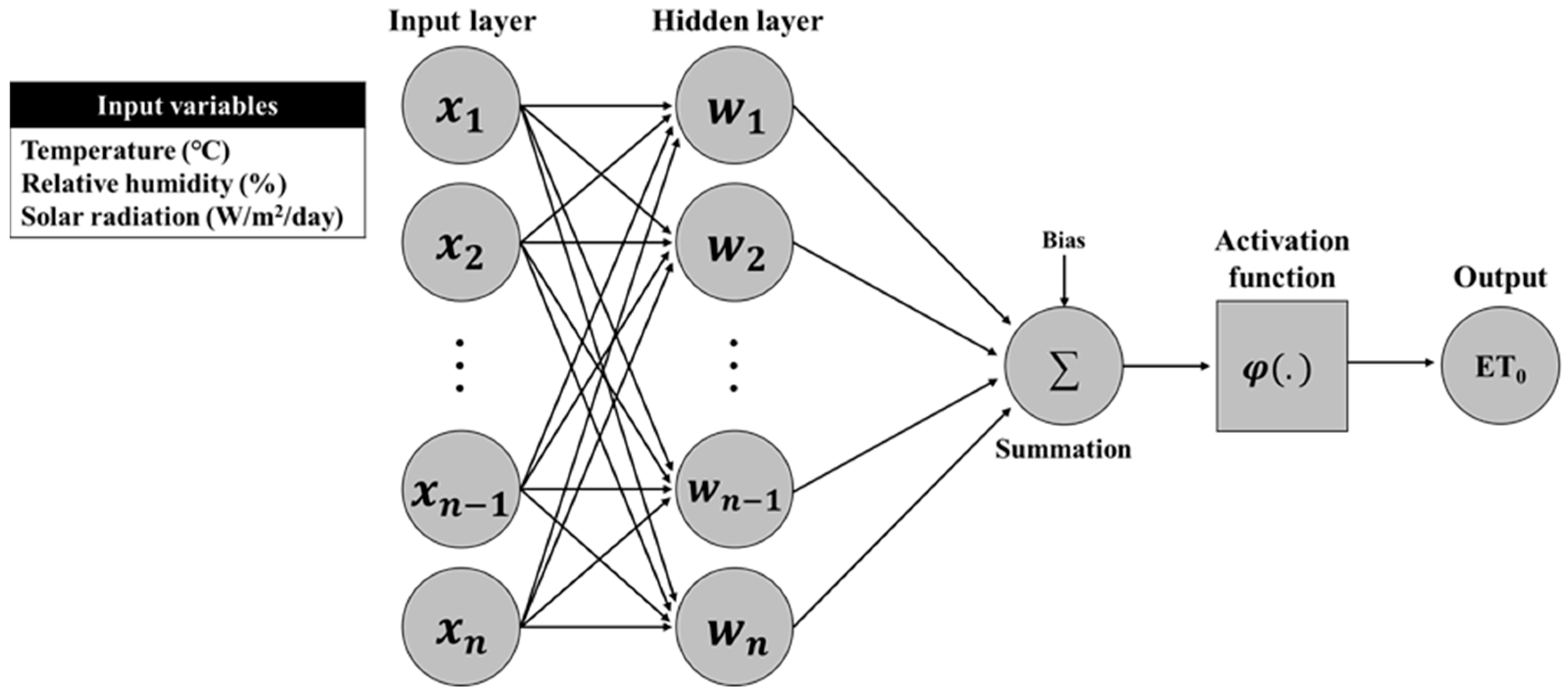
Meteorological variables that are readily accessible and reliably measured can be used to estimate the lacking meteorological variables required for the PM equation. When the observed RH data are unattainable, the ea can be estimated by Equation (10). Equation (11) offers an estimation method for Rs in the absence of observed radiation data. The regional or global average wind speed (2 m/s) can be used as a substitute when the u2 is not measured [33,38].
E a = 0.611 × e x p ( 17.27 T m i n T m i n + 237.3 )
R s = k R s R a ( T m a x T m i n )
where ea is the actual vapor pressure (kPa); Tmin and Tmax are the minimum and maximum temperature (°C), respectively; kRs denotes the adjustment coefficient that needs to be locally calibrated; and Ra represents extraterrestrial radiation (MJ/m2/day) calculated by Equation (9).
This study used 28-year meteorological data to calibrate the average wind speed (used to substitute the u2) and kRs (required to estimate Rs), which are specific for each geographic region (Table 2). The different values in each geographic region reflect the distinction in climate conditions among the four regions.

2.3.3. ANN Models

The typical ANN architecture comprises an input layer for data introduction, one or more hidden layers for data processing, and an output layer for generating the final results [17]. The basic operation of ANN is as follows: initially, data are inputted into the network’s input layer, where each input variable is represented by a neuron. Subsequently, the information in each neuron is weighted and summed, with the resulting weighted sum serving as input for the subsequent layer. Finally, the output is converted through an activation function such as the logistic and hyperbolic tangent commonly used in hydrological research [19]. After the model is constructed, the ANN measures the difference between the model output and the reference value through a loss function, iteratively adjusting the weights until it finds a set of weights that minimize the loss function value.
This study employed feed-forward multilayer perceptron ANNs and an Adam training algorithm. The ratio of training data commonly used in machine learning is 60% to 80% [10,16,31]; therefore, the 28 years of daily data from each meteorological station were randomly split into three parts for model training (70%), validation (15%), and testing (15%), respectively. The training set was used to develop the ANN model and optimize the model parameters. The validation set served to assess overfitting during the training stage, and the testing set evaluated the generalizability of the developed model. Next, data from all stations within the same geographic region were pooled to construct ANN models for each region.
The following hyperparameter combinations were evaluated: the number of epochs was 50, and the batch size was 32. The hyperbolic tangent function was used as an activation function [19], and the type of loss function was the mean square error. The model becomes more complex as the number of hidden layers and units increases, thereby increasing the computational cost and causing overfitting. Additionally, increasing the number of neurons is not always good [39]; therefore, this study assessed the number of hidden layers ranging from 1 to 3 layers and the number of hidden units ranging from 10 to 200 with a step size of 10. The learning rate was set to 0.001. Additionally, a patience value of 5 was set [40,41], indicating that if there is no improvement in the validation error after 5 epochs, the training process would be stopped to prevent overfitting. The T, RH, and Rs were used as input variables, and the PM-calculated ET0 was the output variable (Figure 2). The input variables were standardized using Equation (12) to ensure a uniform contribution from each feature before training and testing [31,42]. Four combinations of input variables were explored: (1) T, (2) T and Rs, (3) T and RH, and (4) T, Rs, and RH. The ANNs were implemented using Tensorflow2.6 based on Python (version 3.7), and the standardization was implemented using the StandardScaler function in the sklearn.preprocessing package based on the scikit-learn module. The best combination of the number of hidden layers and hidden units was determined by grid search. The final hyperparameter configurations of the ANN models using different input variable combinations for each geographic region are summarized in Table 3. The data are standardized as follows:
x s = x o x ¯ S D
where x o and x s are values before and after the standardization, respectively. x ¯ and SD are the mean and standard deviation of the data, respectively.

2.4. Short-Term Forecasting Daily ET0 under Variable-Limited Conditions

Since LSTM can capture and model temporal dependencies, it is widely used for processing time-series data [43]. A neuron in the LSTM model comprises a cell state and three gates: the input gate ( i t ), forget gate ( f t ), and output gate ( O t ), enabling selective retention or modification of information. The general LSTM structure is shown in Figure 3a and its computing steps can be described as the following equations:
i t = σ W i · h t 1 , x t + b i
f t = σ ( W f · h t 1 , x t + b f )
C ~ t = t a n h ( W C · h t 1 , x t + b C )
C t = f t     C t 1 + i t     C ~ t
O t = σ ( W o · h t 1 , x t + b o )
h t = O t     t a n h ( C t )
where C ~ t is the cell state candidate; C t denotes the new cell state; h t is the hidden state vector; x t represents the input vector; W i , W f , W C , and W o stand for the weight matrices; b i , b f , b C , and b o are the bias vectors; σ ( · ) is the sigmoid function; t a n h ( · ) represents the hyperbolic tangent function; and denotes the element-wise product [31,40,44].
In CNN-LSTM architecture, the convolution layer is employed for extracting features from input data, and the extracted features are subsequently fed into LSTM layers for processing information with sequential features. The convolution layers extract salient features automatically, with a one-dimensional (1D) convolutional layer typically used for sequential data or time series [26]. In the CNN-LSTM model, an input layer is followed by a 1D convolutional layer; subsequently, the output of the convolutional layer undergoes further processing through LSTM layers, and finally, the model concludes with an output layer in the form of a dense layer.
A 90%–5%–5% split [40] was used to allow the models to learn complex patterns, so the 28 years of daily data from each meteorological station were sequentially divided into three parts: training (1 January 1995 to 13 March 2020), validation (14 March 2020 to 6 August 2021), and testing (7 August 2021 to 31 December 2022). Subsequently, the data of all stations belonging to the same geographic region were pooled to construct ET0 forecasting models for each region. In this study, the past meteorological variables were used as inputs to forecast four-day-ahead ET0, and three combinations of input variables were examined: (1) T and Rs, (2) T and RH, and (3) T, Rs, and RH. A standardization process (Equation (12)) was used to ensure an equal contribution from each feature. The model structure comprised one 1D convolution layer, one 1D max pooling layer, one to three LSTM layers, and one densely connected NN layer (Figure 3b). The following hyperparameter combinations were evaluated: the number of epochs was 50, and the batch size was 32. The hyperbolic tangent function was used as the activation function [19], and the mean square error was used as the loss function. The number of hidden units was set from 10 to 200 with a step size of 10, the learning rate was set to 0.001, and the optimizer used the Adam algorithm. This study chose a 90%–5%–5% split percentage to establish models, but this extreme split could increase the risk of overfitting. Therefore, a dropout rate of 0.4 [40] and a patience value of 5 for early stopping [40,41] were set to prevent overfitting. The models were developed using Tensorflow2.6 based on Python (version 3.7), and the standardization was implemented using the StandardScaler function. In this study, the best combination of the number of hidden layers and hidden units was determined by grid search. The final hyperparameter configurations for the LSTM and CNN-LSTM models using different combinations of input variables for each geographic region are summarized in Table 4.

2.5. Performance Comparison Criteria

The performance of each method was evaluated using three standard statistical metrics: the r, mean absolute error (MAE), and root mean square error (RMSE). The value of r ranges between 1 and 1, serving as an indicator to evaluate the linear relationship between the predicted and observed values. MAE and RMSE quantify the bias between the predicted value and the observed value, with values ranging from 0 to infinity. A higher r, along with a lower MAE and RMSE, signifies a more accurate prediction.
r = i = 1 n o i o ¯ p i p ¯ i = 1 n o i o ¯ 2 i = 1 n ( p i p ¯ ) 2
M A E = i = 1 n o i p i n
R M S E = i = 1 n ( o i p i ) 2 n
where n is the number of observations in the testing set for the AI algorithms (ANN, LSTM, and CNN-LSTM) and the total number of 28-year data for other methods; o i is the observed value (the PM-calculated ET0); p i is the predicted (estimated or forecasted) ET0 value by the other methods; and o ¯ and p ¯ are the mean of o i and p i , respectively.

3. Results and Discussion

3.1. Evaluation of ET0 Estimation Approaches under Variable-Limited Conditions

3.1.1. Performance of ET0 Estimation Methods

This study used 28 years of meteorological data from 18 stations distributed across the four geographic regions of Taiwan to evaluate the efficacy of various ET0 estimation approaches under variable-limited conditions (Table 5). Regarding the alternative equations, the r between HS-estimated ET0 and PM-calculated ET0 ranged from 0.444 to 0.735, with MAE ranging from 0.95 to 1.41 mm/day and RMSE from 1.22 to 1.85 mm/day. For the Makkink equation, the r ranged from 0.972 to 0.990, MAE ranged from 1.33 to 1.93 mm/day, and RMSE ranged from 1.53 to 2.08 mm/day. The Turc equation performed the best among the three PM-alternative equations, with the r ranging from 0.984 to 0.997, MAE ranging from 0.50 to 0.84 mm/day, and RMSE ranging from 0.68 to 1.03 mm/day.
Regarding the RPM approach, it does not perform well when only considering the temperature, i.e., RPM (T), as evidenced by r ranging from 0.357 to 0.735, MAE ranging from 2.12 to 2.87 mm/day, and RMSE ranging from 2.72 to 3.39 mm/day (Table 5). For the combination of two variables, RPM (T, Rs) performed the best, with r ranging from 0.953 to 0.990, MAE ranging from 0.21 to 0.41 mm/day, and RMSE ranging from 0.27 to 0.59 mm/day; in contrast, RPM (T, u2) performed the worst, with r ranging from 0.468 to 0.674, MAE ranging from 2.13 to 2.99 mm/day, and RMSE ranging from 2.72 to 3.47 mm/day. In the RPM model with three variables, the accuracy of estimating ET0 is the worst when the Rs variable is not included in the model, with r of RPM (T, u2, RH) ranging from 0.527 to 0.655, MAE ranging from 2.15 to 2.82 mm/day, and RMSE ranging from 2.76 to 3.28 mm/day. However, the lack of u2 has the most negligible impact on accuracy within the three-variable model, as evidenced by r of RPM (T, Rs, RH) ranging from 0.990 to 0.998, MAE ranging from 0.07 to 0.18 mm/day, and RMSE ranging from 0.12 to 0.27 mm/day.
In terms of the application of ANN to establish the ET0 estimation models, the combinations of (T, Rs) and (T, Rs, RH) demonstrated a favorable performance, with r ranging from 0.977 to 0.998, MAE ranging from 0.07 to 0.30 mm/day, and RMSE ranging from 0.12 to 0.45 mm/day (Table 5). The performance of the proposed ANN models is similar to that of ANN using the same input variables reported in Antonopoulos and Antonopoulos [22]. In addition, the performance of the ANN (T) model is comparable to that of the HS equation, with r ranging from 0.543 to 0.731, MAE ranging from 1.04 to 1.36 mm/day, and RMSE ranging from 1.32 to 1.68 mm/day.

3.1.2. Comparison of Different ET0 Estimation Methods and Inputs Combination

The results in Table 5 revealed that irrespective of the approach employed, using the combination of T, Rs, and RH (e.g., Turc, RPM (T, Rs, RH) and ANN (T, Rs, RH)) achieved the best results, characterized by r above 0.984 with MAE and RMSE values below 0.84 and 1.03 mm/day, respectively. Notably, both RPM (T, Rs, RH) and ANN (T, Rs, RH) slightly outperformed the Turc equation. Conversely, the performance of each approach is poor when only considering the temperature in the model (e.g., HS, RPM (T), and ANN (T)), especially in southern Taiwan. For the case when only temperature data were available, the HS equation and ANN (T) exhibited equally poor performance, but with noticeably lower MAE values compared to RPM (T). Yang et al. [15] conducted a comparison between the HS equation and RPM (T), concluding that the HS equation outperformed RPM in subtropical regions. Similarly, Córdova et al. [45] reported that the HS equation performed slightly better than RPM (T), but still yielded an unsatisfactory result.
The results in Table 5 indicate that accurate ET0 estimates can still be achieved even without u2. Therefore, as mentioned by Córdova et al. [45], the absence of u2 was not a major source of error in humid climates. The role of u2 in ET0 calculation is subject to two main perspectives: some argue that it is a decisive factor due to the potential for measurement errors, while others contend that u2 does not have much impact on ET0 [17]. Nevertheless, Fisher et al. [46] stated that wind speed plays an important role in modeling the complex nonlinear behavior of ET0. Furthermore, Makwana et al. [47] found that the performance of the ANN model could be significantly improved in windy regions by including wind speed and Tmax, with r and MAE values of 0.91 and 0.59 mm/day, respectively.
Temperature and radiation are considered essential inputs to estimate ET0 [22,24]; therefore, including observed Rs in the ET0 calculation generally yields satisfactory results, except that the Makkink equation exhibits higher MAE and RMSE values (Table 5). RH is an important variable in estimating ET0 in humid regions [17], such as Taiwan. Consequently, the Makkink equation, which does not incorporate RH information, performs poorly. However, RPM (T, Rs) also lacks observed RH data, but the information about RH is estimated by Equation (10), hence it can still perform well. Conversely, methods lacking Rs observations perform poorly (Table 5). Even though the RPM approach estimates the absent Rs information through Equation (11), its performance remains unsatisfactory. Córdova et al. [45] observed that estimating Rs based on Equation (11) yielded poor results in humid conditions for the RPM approach. Sentelhas et al. [12] discovered that when the actual Rs falls below 20 MJ/m2/day, Equation (11) tends to systematically overestimate radiation. Given that Taiwan exhibits a humid climate with Rs values less than 20 MJ/m2/day (Table 1), this could account for the suboptimal performance of RPM in this study.
This study aimed to evaluate the effectiveness of ANN in estimating ET0 using limited meteorological variables. Traore et al. [48] noted that the ANN model fed with only temperature data performed better than the HS equation, which included some radiation information by using Ra as inputs. In this study, the ANN (T) model yielded r ranging from 0.543 to 0.731, MAE ranging from 1.04 to 1.36 mm/day, and RMSE ranging from 1.32 to 1.68 mm/day (Table 5). Notably, the ANN (T) model exhibited superior performance compared to RPM (T) and demonstrated comparable efficacy to the HS equation. In scenarios involving two input variables, the ANN (T, RH) model exhibited r ranging from 0.710 to 0.828, MAE ranging from 0.87 to 1.12 mm/day, and RMSE ranging from 1.12 to 1.40 mm/day; the ANN (T, RH) performed better than RPM (T, RH). On the other hand, the ANN (T, Rs) model demonstrated r ranging from 0.977 to 0.991, MAE ranging from 0.19 to 0.30 mm/day, and RMSE ranging from 0.25 to 0.45 mm/day, surpassing both RPM (T, Rs) and the Makkink equation. When T, RH, and Rs data are available, the ANN (T, Rs, RH) model exhibited r ranging from 0.992 to 0.998, MAE ranging from 0.07 to 0.16 mm/day, and RMSE ranging from 0.12 to 0.25 mm/day. The ANN (T, Rs, RH) model performed better than the Turc equation and showed comparable performance to RPM (T, Rs, RH). These findings underscore the superior performance of ANN models compared to traditional methods utilizing the same inputs. Additionally, the performance of ANN using T and Rs as input variables is comparable with the models using more input variables, as mentioned by Jain et al. [49].

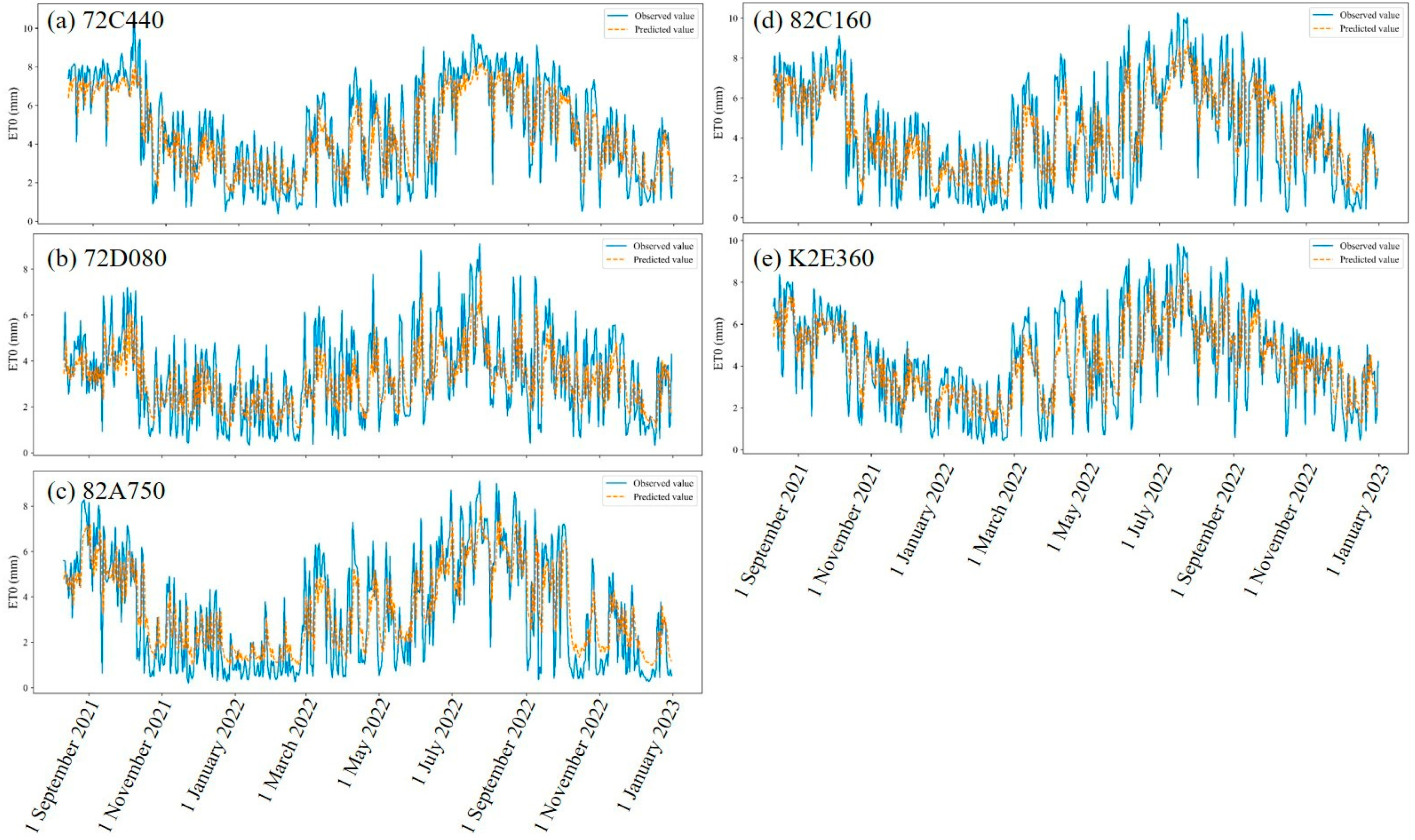
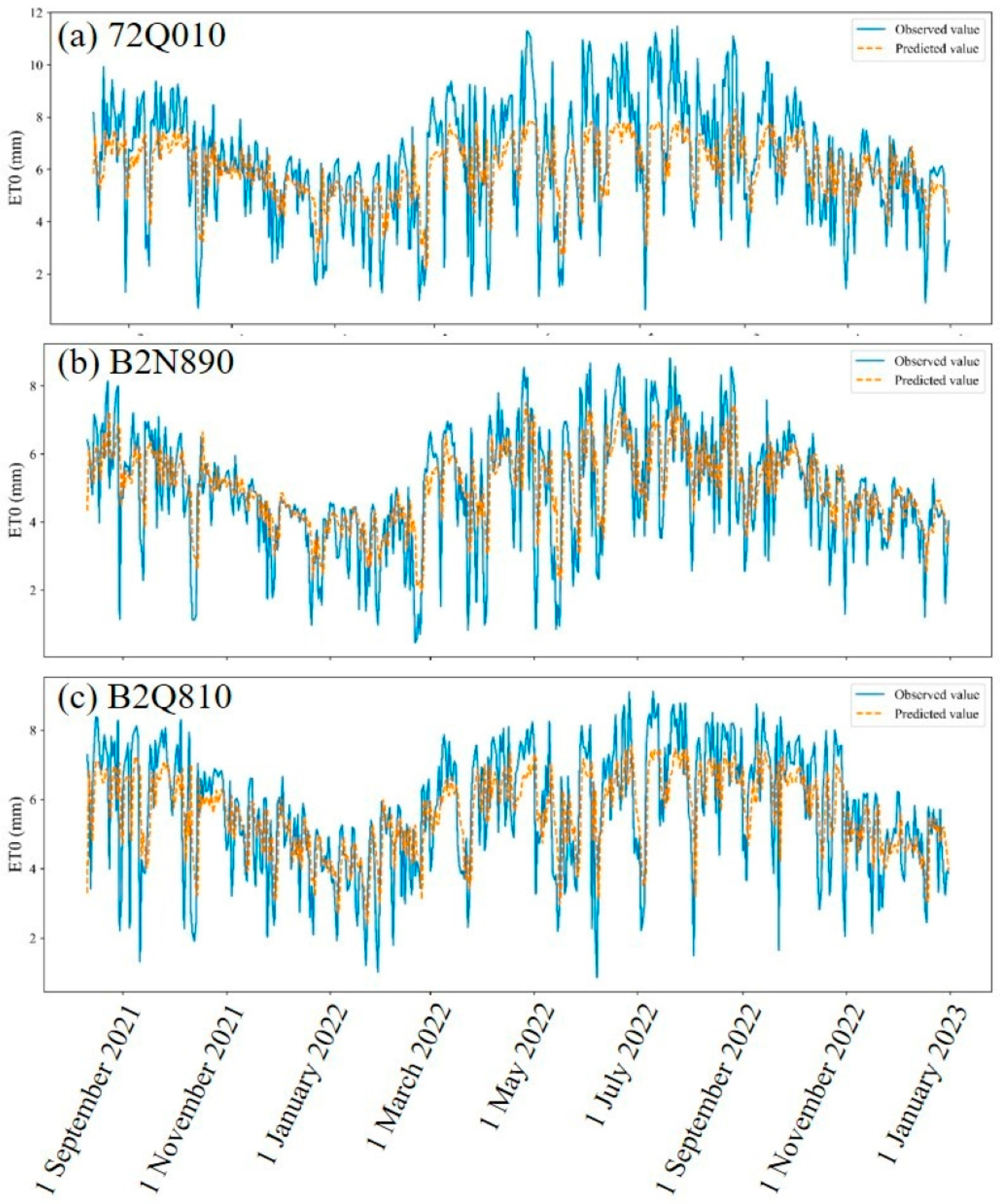
3.2. Performance of AI Algorithms for the Short-Term Forecasting ET0 with Limited Variables

This study used 28 years of meteorological data from 18 stations in four geographic regions of Taiwan to construct LSTM and CNN-LSTM models for short-term ET0 forecasting with limited meteorological variables. When considering scenarios with two input variables, the LSTM (T, RH) model exhibited an r ranging from 0.159 to 0.711, MAE ranging from 1.29 to 1.60 mm/day, and RMSE ranging from 1.60 to 2.01 mm/day (Table 6). Notably, the LSTM (T, RH) performed better than CNN-LSTM (T, RH) in the majority of regions. Similarly, the LSTM (T, Rs) model yielded the values of r ranging from 0.609 to 0.755, MAE ranging from 1.04 to 1.31 mm/day, and RMSE ranging from 1.35 to 1.62 mm/day, outperforming the CNN-LSTM (T, Rs) model. Considering T, RH, and Rs data simultaneously, the LSTM (T, Rs, RH) model attained the values of r ranging from 0.608 to 0.756, MAE ranging from 1.05 to 1.28 mm/day, and RMSE ranging from 1.35 to 1.62 mm/day, exhibiting a superior performance compared to the CNN-LSTM (T, Rs, RH) model (Table 6). Moreover, the performance of the proposed models was consistent between the training (Table S1) and testing phases (Table 6) indicating that overfitting did not occur.
For CNN-LSTM models, the expectation is that CNN layers can extract features from input data, while LSTM layers can capture time patterns to enhance the model’s capability and achieve higher performance. However, in the present study, the CNN-LSTM models performed worse than the LSTM models. This finding contrasts with those of Barzegar et al. [50] and Yin et al. [31], who reported that integrated or hybridized algorithms outperformed standalone algorithms for ET0 forecasting. Moreover, while hybrid algorithms can enhance the model performance, the extent of improvement may not always be substantial [51]. Additionally, hybrid algorithms typically necessitate tuning more hyperparameters, making them time-consuming during model deployment [17]. Zhang et al. [16] compared LSTM to three novel AI models and found that the LSTM model marginally outperformed in short-term daily ET0 forecasting across diverse climate conditions. Considering the computational efficiency and model performance, the LSTM (T, Rs, RH) was regarded as the best structure in this study.
In evaluating the LSTM (T, Rs, RH) model across various geographic regions for forecasting four-day-ahead ET0 at each meteorological station, the overall trend of the daily ET0 forecasting was consistent with the daily ET0 values calculated by the PM equation (Figure 4, Figure 5, Figure 6 and Figure 7), underscoring the forecasting ability of proposed models. During the test period lasting more than one year, the disparity between the cumulative ET0 forecasted by the LSTM (T, Rs, RH) model and the observed ET0 ranged from 166.05 to 68.12 mm, with most differences within ± 5%, except for stations 72D080 and 72S590 (Table 7). The poor performance of the forecasting models at these two stations may be due to their differing meteorological characteristics from most stations in the same region (Table 1). Interestingly, there was a large difference between predicted and observed values in autumn (September–November) (Figure 4, Figure 5, Figure 6 and Figure 7), which is different from the previous studies that reported that winter and summer were more prone to forecasting errors [52,53]. This might be due to Taiwan’s climate conditions suffering the large meteorological fluctuations affected by typhoons, southwest monsoons, and northeast monsoons [54]. The model performance could be increased by using the day of the year as an additional input variable [26] to provide information about seasons or grouping the data into different seasons to establish a specific model for each season [55]. Future studies should explore these strategies to refine ET0 forecasting models.

3.3. Advantages and Limitations of the Proposed Models

This study shows that the AI algorithm can sufficiently estimate and even forecast ET0 using only a few meteorological variables but its forecasting capabilities could be improved and tested over longer periods to increase the reliability. Many studies caution that AI models remain empirical, implying that a model developed for one location may not generalize well to the other locations [16,19]. Increasing the data variability for modeling may increase the generalizability of AI models [10,19]. This study developed ET0 estimating and forecasting models in regional scenarios, i.e., trained with pooled data from several meteorological stations, to achieve a higher generalization capacity. These regional models are more readily applicable in practical settings, as a single model can suffice for an entire region. However, previous studies pointed out that the regional models exhibit lower accuracy than those developed in localized scenarios due to dissimilarities in the training data [10,19,56]. To consider the generalizability and performance, the stations could be grouped based on meteorological characteristics rather than geographical locations, and then a specific model was built for each cluster [10,57]. This strategy is expected to improve the performance of proposed regional models at specific stations.
It must be mentioned that the ANN and LSTM endeavor to mimic the underlying evapotranspiration process through the link weights and thresholds. However, the black-box nature of these models impedes their ability to elucidate the relationship between input and output through explicit expressions [17,19]. Consequently, they cannot supplant physical mechanisms [16,19]. In addition, climate change affects evapotranspiration, not only in Taiwan [58,59] but also in other regions [60,61,62,63,64,65,66,67] worldwide. Consequently, a “fixed” forecasting model may not make accurate predictions in the future [17], so the forecasting models should be trained with long-term data and continuously adjusted by incorporating new data through dynamic modeling [17,68]. Furthermore, greenhouse cultivation is rapidly growing and as the water demand cannot be met through rainfall, it must be supplied through irrigation. However, irrigation in greenhouses is often based on a fixed schedule or the grower’s experience, often leading to insufficient irrigation or excessive waste of water resources [69]. Utilizing evapotranspiration information to determine the appropriate timing and amount of irrigation can greatly enhance the precision of greenhouse cultivation. Most studies estimated or forecasted evapotranspiration under open-field conditions [70], but applying these models to greenhouse environments resulted in discrepancies due to the vastly different conditions [70,71]; therefore, future studies should focus more on estimating and forecasting evapotranspiration within greenhouses.

4. Conclusions

Since ET0 is related to the quantification of crop water demand, the information on ET0 is useful for irrigation planning and water resources management. However, the standard method for calculating ET0, the PM equation, is primarily limited by the costs associated with collecting numerous meteorological parameters. Considering that AI algorithms are known for modeling complex relationships without requiring an in-depth understanding of underlying physical processes, they have great potential to obtain ET0 information with fewer variables. The results of this study revealed that ANN models outperformed the traditional methods (RPM and PM-alternative equations) with the same inputs for ET0 estimation. Particularly, the ANN (T, Rs, RH) exhibited the highest accuracy (r was 0.992 to 0.998, MAE was 0.07 to 0.16 mm/day, and RMSE was 0.12 to 0.25 mm/day), while the ANN utilizing T and Rs yielded satisfactory results (r was 0.977 to 0.991, MAE was 0.19 to 0.30 mm/day, and RMSE was 0.25 to 0.45 mm/day). For the short-term ET0 forecasting, LSTM models performed better than CNN-LSTM models, with LSTM (T, Rs, RH) demonstrating the best performance in forecasting four-day-ahead ET0 (r ranging from 0.608 to 0.756, MAE ranging from 1.05 to 1.28 mm/day, and RMSE ranging from 1.35 to 1.62 mm/day). Over the one-year test period, the error percentage of LSTM (T, Rs, RH) models was within ± 5% for most meteorological stations but these models can be tested over longer periods to increase their reliability. Moreover, the forecasting capabilities can be further improved by using the day of the year as an additional input variable or grouping/clustering data. As the proposed ANN and LSTM models were developed in regional and variable-limited scenarios, they offer practical utility across the entire region without necessitating the inclusion of all meteorological variables. In addition, these models may be applied to other regions that have similar conditions to Taiwan. Future studies can focus more on estimating and forecasting evapotranspiration within greenhouses. Additionally, it is important to consider the impact of climate change. Accurate ET0 estimation and forecasting models enable the agricultural sector to determine irrigation water requirements promptly or in advance. As the models are refined and their applicability is expanded, they could significantly benefit precise water managing and irrigation scheduling in crop production.

Supplementary Materials

The following supporting information can be downloaded at: https://0-www-mdpi-com.brum.beds.ac.uk/article/10.3390/agriculture14040510/s1, Table S1. Training performance of short-term ET0 forecasting models in each geographic region. Bold characters indicate better results among the models.

Author Contributions

Conceptualization, S.-L.F.; Data curation, S.-L.F., Y.-S.L., S.-C.C., Y.-L.C. and B.-Y.T.; Funding acquisition, B.-J.K.; Investigation, S.-L.F., S.-C.C., Y.-L.C. and B.-Y.T.; Methodology, S.-L.F. and Y.-S.L.; Writing—original draft, S.-L.F. and Y.-S.L.; Writing—review & editing, B.-J.K. All authors have read and agreed to the published version of the manuscript.

Funding

This work was financially supported by NSTC 112-2634-F-005-002—project Smart Sustainable New Agriculture Research Center (SMARTer).

Data Availability Statement

The original contributions presented in the study are included in the article, further inquiries can be directed to the corresponding author.

Conflicts of Interest

The authors declare no conflicts of interest.

Abbreviations

AIArtificial intelligence
ANNArtificial neural network
CNN-LSTMConvolution neural network long- short-term memory
eaActual vapor pressure
ET0Reference evapotranspiration
HS equationHargreaves-Samani equation
LSTMLong short-term memory
MAEMean absolute error
PM equationPenman-Monteith equation
rCorrelation coefficient
RaExtraterrestrial radiation
RsSolar radiation
RMSERoot mean square error
RHRelative humidity
RPMReduced-set Penman-Monteith
TMean air temperature
TmaxMaximum temperature
u2Mean wind speed at 2 m above ground

References

  1. Sharma, V.; Irmak, S. Mapping spatially interpolated precipitation, reference evapotranspiration, actual crop evapotranspiration, and net irrigation requirements in Nebraska: Part I. Precipitation and reference evapotranspiration. Trans. ASABE 2012, 55, 907–921. [Google Scholar] [CrossRef]
  2. Sharma, V.; Irmak, S. Mapping spatially interpolated precipitation, reference evapotranspiration, actual crop evapotranspiration, and net irrigation requirements in Nebraska: Part II. Actual crop evapotranspiration and net irrigation requirements. Trans. ASABE 2012, 55, 923–936. [Google Scholar] [CrossRef]
  3. Rahman, M.A.; Ali, M.; Mojid, M.A.; Anjum, N.; Haq, M.E.; Kainose, A.; Dissanayaka, K.D.C.R. Crop coefficient, reference crop evapotranspiration and water demand of dry-season Boro rice as affected by climate variability: A case study from northeast Bangladesh. Irrig. Drain. 2023, 72, 148–165. [Google Scholar] [CrossRef]
  4. Dai, A. Characteristics and trends in various forms of the Palmer Drought Severity Index during 1900–2008. J. Geophys. Res. 2011, 116, D12115. [Google Scholar] [CrossRef]
  5. Paulo, A.A.; Rosa, R.D.; Pereira, L.S. Climate trends and behavior of drought indices based on precipitation and evapotranspiration in Portugal. Nat. Hazards Earth Syst. Sci. 2012, 12, 1481–1491. [Google Scholar] [CrossRef]
  6. McEvoy, D.J.; Huntington, J.L.; Abatzoglou, J.T.; Edwards, L.M. An evaluation of multi-scalar drought indices in Nevada and Eastern California. Earth Interact. 2012, 16, 1–18. [Google Scholar] [CrossRef]
  7. Allen, R.G.; Pereira, L.S.; Raes, D.; Smith, M. Crop Evapotranspiration: Guidelines for Computing Crop Water Requirements; FAO: Rome, Italy, 1998; Volume 56. [Google Scholar]
  8. Allen, R.G.; Pereira, L.S.; Howell, T.A.; Jensen, M.E. Evapotranspiration information reporting: I. Factors governing measurement accuracy. Agric. Water Manag. 2011, 98, 899–920. [Google Scholar] [CrossRef]
  9. Landeras, G.; Ortiz-Barredo, A.; López, J.J. Comparison of artificial neural network models and empirical and semi-empirical equations for daily reference evapotranspiration estimation in the Basque Country (Northern Spain). Agric. Water Manag. 2008, 95, 553–565. [Google Scholar] [CrossRef]
  10. Ferreira, L.B.; da Cunha, F.F.; de Oliveira, R.A.; Fernandes Filho, E.I. Estimation of reference evapotranspiration in Brazil with limited meteorological data using ANN and SVM—A new approach. J. Hydrol. 2019, 572, 556–570. [Google Scholar] [CrossRef]
  11. Cai, J.B.; Liu, Y.; Lei, T.W.; Pereira, L.S. Estimating reference evapotranspiration with the FAO Penman-Monteith equation using daily weather forecast messages. Agric. For. Meteorol. 2007, 145, 22–35. [Google Scholar] [CrossRef]
  12. Sentelhas, P.C.; Gillespie, T.J.; Santos, E.A. Evaluation of FAO Penman-Monteith and alternative methods for estimating reference evapotranspiration with missing data in Southern Ontario, Canada. Agric. Water Manag. 2010, 97, 635–644. [Google Scholar] [CrossRef]
  13. Pereira, L.S.; Allen, R.G.; Smith, M.; Raes, D. Crop evapotranspiration estimation with FAO56: Past and future. Agric. Water Manag. 2015, 147, 4–20. [Google Scholar] [CrossRef]
  14. Tabari, H.; Talaee, P.H. Local calibration of the Hargreaves and Priestley-Taylor equations for estimating reference evapotranspiration in arid and cold climates of Iran based on the Penman-Monteith model. J. Hydrol. Eng. 2011, 16, 837–845. [Google Scholar] [CrossRef]
  15. Yang, Y.; Cui, Y.; Bai, K.; Luo, T.; Dai, J.; Wang, W.; Luo, Y. Short-term forecasting of daily reference evapotranspiration using the reduced-set Penman-Monteith model and public weather forecasts. Agric. Water Manag. 2019, 211, 70–80. [Google Scholar] [CrossRef]
  16. Zhang, L.; Zhao, X.; Zhu, G.; He, J.; Chen, J.; Chen, Z.; Traore, S.; Liu, J.; Singh, V.P. Short-term daily reference evapotranspiration forecasting using temperature-based deep learning models in different climate zones in China. Agric. Water Manag. 2023, 289, 108498. [Google Scholar] [CrossRef]
  17. Goyal, P.; Kumar, S.; Sharda, R. A review of the Artificial Intelligence (AI) based techniques for estimating reference evapotranspiration: Current trends and future perspectives. Comput. Electron. Agric. 2023, 209, 107836. [Google Scholar] [CrossRef]
  18. Wen, X.; Si, J.; He, Z.; Wu, J.; Shao, H.; Yu, H. Support-vector-machine-based models for modeling daily reference evapotranspiration with limited climatic data in extreme arid regions. Water Resour. Manag. 2015, 29, 3195–3209. [Google Scholar] [CrossRef]
  19. Kumar, M.; Raghuwanshi, N.S.; Singh, R. Artificial neural networks approach in evapotranspiration modeling: A review. Irrig. Sci. 2011, 29, 11–25. [Google Scholar] [CrossRef]
  20. Adeloye, A.J.; Rustum, R.; Kariyama, I.D. Neural computing modeling of the reference crop evapotranspiration. Environ. Model. Softw. 2012, 29, 61–73. [Google Scholar] [CrossRef]
  21. Tikhamarine, Y.; Malik, A.; Souag-Gamane, D.; Kisi, O. Artificial intelligence models versus empirical equations for modeling monthly reference evapotranspiration. Environ. Sci. Pollut. Res. 2020, 27, 30001–30019. [Google Scholar] [CrossRef]
  22. Antonopoulos, V.Z.; Antonopoulos, A.V. Daily reference evapotranspiration estimates by artificial neural networks technique and empirical equations using limited input climate variables. Comput. Electron. Agric. 2017, 132, 86–96. [Google Scholar] [CrossRef]
  23. Chen, Z.; Zhu, Z.; Jiang, H.; Sun, S. Estimating daily reference evapotranspiration based on limited meteorological data using deep learning and classical machine learning methods. J. Hydrol. 2020, 591, 125286. [Google Scholar] [CrossRef]
  24. Sharma, G.; Singh, A.; Jain, S. A hybrid deep neural network approach to estimate reference evapotranspiration using limited climate data. Neural Comput. Applic. 2022, 34, 4013–4032. [Google Scholar] [CrossRef]
  25. Xing, L.; Cui, N.; Guo, L.; Du, T.; Gong, D.; Zhan, C.; Zhao, L.; Wu, Z. Estimating daily reference evapotranspiration using a novel hybrid deep learning model. J. Hydrol. 2022, 614, 128567. [Google Scholar] [CrossRef]
  26. Ferreira, L.B.; da Cunha, F.F. Multi-step ahead forecasting of daily reference evapotranspiration using deep learning. Comput. Electron. Agric. 2020, 178, 105728. [Google Scholar] [CrossRef]
  27. Luo, Y.; Chang, X.; Peng, S.; Khan, S.; Wang, W.; Zheng, Q.; Cai, X. Short-term forecasting of daily reference evapotranspiration using the Hargreaves–Samani model and temperature forecasts. Agric. Water Manag. 2014, 136, 42–51. [Google Scholar] [CrossRef]
  28. Karbasi, M. Forecasting of multi-step ahead reference evapotranspiration using wavelet-Gaussian process regression model. Water Resour. Manag. 2018, 32, 1035–1052. [Google Scholar] [CrossRef]
  29. Perera, K.C.; Western, A.W.; Nawarathna, B.; George, B. Forecasting daily reference evapotranspiration for Australia using numerical weather prediction outputs. Agric. Forest Meteorol. 2014, 194, 50–63. [Google Scholar] [CrossRef]
  30. Roy, D.K.; Sarkar, T.K.; Kamar, S.S.A.; Goswami, T.; Muktadir, M.A.; Al-Ghobari, H.M.; Alataway, A.; Dewidar, A.Z.; El-Shafei, A.A.; Mattar, M.A. Daily prediction and multi-step forward forecasting of reference evapotranspiration using LSTM and Bi-LSTM models. Agronomy 2022, 12, 594. [Google Scholar] [CrossRef]
  31. Yin, J.; Deng, Z.; Ines, A.V.M.; Wu, J.; Rasu, E. Forecast of short-term daily reference evapotranspiration under limited meteorological variables using a hybrid bi-directional long short-term memory model (Bi-LSTM). Agric. Water Manag. 2020, 242, 106386. [Google Scholar] [CrossRef]
  32. Narapusetty, B.; DelSole, T.; Tippett, M.K. Optimal estimation of the climatological mean. J. Clim. 2009, 22, 4845–4859. [Google Scholar] [CrossRef]
  33. McMahon, T.A.; Peel, M.C.; Lowe, L.; Srikanthan, R.; McVicar, T.R. Estimating actual, potential, reference crop and pan evaporation using standard meteorological data: A pragmatic synthesis. Hydrol. Earth Syst. Sci. 2013, 17, 1331–1363. [Google Scholar] [CrossRef]
  34. Zotarelli, L.; Dukes, M.D.; Romero, C.C.; Migliaccio, K.W.; Morgan, K.T. Step by Step Calculation of the Penman-Monteith Evapotranspiration (FAO-56 Method); Institute of Food and Agricultural Sciences, University of Florida: Gainesville, FL, USA, 2010; Volume AE459, pp. 1–10. [Google Scholar]
  35. Vicente-Serrano, S.M.; Azorin-Molina, C.; Sanchez-Lorenzo, A.; Revuelto, J.; López-Moreno, J.I.; González-Hidalgo, J.C.; Moran-Tejeda, E.; Espejo, F. Reference evapotranspiration variability and trends in Spain, 1961–2011. Glob. Planet. Change 2014, 121, 26–40. [Google Scholar] [CrossRef]
  36. Hargreaves, G.H.; Samani, Z.A. Reference crop evapotranspiration from temperature. Appl. Eng. Agric. 1985, 1, 96–99. [Google Scholar] [CrossRef]
  37. De Bruin, H.A.R.; Lablans, W.N. Reference crop evapotranspiration determined with a modified Makkink equation. Hydrol. Process. 1998, 12, 1053–1062. [Google Scholar] [CrossRef]
  38. Valiantzas, J.D. Simplified forms for the standardized FAO-56 Penman-Monteith reference evapotranspiration using limited weather data. J. Hydrol. 2013, 505, 13–23. [Google Scholar] [CrossRef]
  39. Kuo, C.-E.; Chen, G.-T. Automatic sleep staging based on a hybrid stacked LSTM neural network: Verification using large-scale dataset. IEEE Access 2020, 8, 111837–111849. [Google Scholar] [CrossRef]
  40. Lin, Y.-S.; Fang, S.-L.; Kang, L.; Chen, C.-C.; Yao, M.-H.; Kuo, B.-J. Combining recurrent neural network and sigmoid growth models for short-term temperature forecasting and tomato growth prediction in a plastic greenhouse. Horticulturae 2024, 10, 230. [Google Scholar] [CrossRef]
  41. Wunsch, A.; Liesch, T.; Broda, S. Groundwater level forecasting with artificial neural networks: A comparison of long short-term memory (LSTM), convolutional neural networks (CNNs), and non-linear autoregressive networks with exogenous input (NARX). Hydrol. Earth Syst. Sci. 2021, 25, 1671–1687. [Google Scholar] [CrossRef]
  42. Rahimi Khoob, A. Comparative study of Hargreaves’s and artificial neural network’s methodologies in estimating reference evapotranspiration in a semiarid environment. Irrig. Sci. 2008, 26, 253–259. [Google Scholar] [CrossRef]
  43. Greff, K.; Srivastava, R.K.; Koutník, J.; Steunebrink, B.R.; Schmidhuber, J. LSTM: A search space odyssey. IEEE Trans. Neural Netw. Learn. Syst. 2016, 28, 2222–2232. [Google Scholar] [CrossRef] [PubMed]
  44. Hochreiter, S.; Schmidhuber, J. Long short-term memory. Neural Comput. 1997, 9, 1735–1780. [Google Scholar] [CrossRef] [PubMed]
  45. Córdova, M.; Carrillo-Rojas, G.; Crespo, P.; Wilcox, B.; Célleri, R. Evaluation of the Penman-Monteith (FAO 56 PM) method for calculating reference evapotranspiration using limited data. Mt. Res. Dev. 2015, 35, 230–239. [Google Scholar] [CrossRef]
  46. Fisher, J.B.; Terry, A.; DeBiase, A.; Qi1, Y.; Xu, M.; Allen, H. Evapotranspiration models compared on a Sierra Nevada forest ecosystem. Environ. Model. Softw. 2005, 20, 783–796. [Google Scholar] [CrossRef]
  47. Makwana, J.J.; Tiwari, M.K.; Deora, B.S. Development and comparison of artificial intelligence models for estimating daily reference evapotranspiration from limited input variables. Smart Agric. Technol. 2023, 3, 100115. [Google Scholar] [CrossRef]
  48. Traore, S.; Wang, Y.-M.; Kerh, T. Artificial neural network for modeling reference evapotranspiration complex process in Sudano-Sahelian zone. Agric. Water Manag. 2010, 97, 707–714. [Google Scholar] [CrossRef]
  49. Jain, S.K.; Nayak, P.C.; Sudheer, K.P. Models for estimating evapotranspiration using artificial neural networks, and their physical interpretation. Hydrol. Process. An Int. J. 2008, 22, 2225–2234. [Google Scholar] [CrossRef]
  50. Barzegar, R.; Aalami, M.T.; Adamowski, J. Short-term water quality variable prediction using a hybrid CNN–LSTM deep learning model. Stoch. Environ. Res. Risk Assess. 2020, 34, 415–433. [Google Scholar] [CrossRef]
  51. Wu, T.; Zhang, W.; Jiao, X.; Guo, W.; Hamoud, Y.A. Evaluation of stacking and blending ensemble learning methods for estimating daily reference evapotranspiration. Comput. Electron. Agric. 2021, 184, 106039. [Google Scholar] [CrossRef]
  52. Bellido-Jimenez, J.A.; Estevez, J.; Garcia-Marin, A.P. New machine learning approaches to improve reference evapotranspiration estimates using intra-daily temperature-based variables in a semi-arid region of Spain. Agric. Water Manag. 2021, 245, 106558. [Google Scholar] [CrossRef]
  53. Bellido-Jimenez, J.A.; Estevez, J.; Garcia-Marin, A.P. A regional machine learning method to outperform temperature-based reference evapotranspiration estimations in Southern Spain. Agric. Water Manag. 2022, 274, 107955. [Google Scholar] [CrossRef]
  54. Su, Y.-C.; Kuo, B.-J. Risk assessment of rice damage due to heavy rain in Taiwan. Agriculture 2023, 13, 630. [Google Scholar] [CrossRef]
  55. Esparza-Gómez, J.M.; Luque-Vega, L.F.; Guerrero-Osuna, H.A.; Carrasco-Navarro, R.; García-Vázquez, F.; Mata-Romero, M.E.; Olvera-Olvera, C.A.; Carlos-Mancilla, M.A.; Solís-Sánchez, L.O. Long short-term memory recurrent neural network and extreme gradient boosting algorithms applied in a greenhouse’s internal temperature prediction. Appl. Sci. 2023, 13, 12341. [Google Scholar] [CrossRef]
  56. Shiri, J.; Nazemi, A.H.; Sadraddini, A.A.; Landeras, G.; Kisi, O.; Fard, A.F.; Marti, P. Comparison of heuristic and empirical approaches for estimating reference evapotranspiration from limited inputs in Iran. Comput. Electron. Agric. 2014, 108, 230–241. [Google Scholar] [CrossRef]
  57. Jato-Espino, D.; Charlesworth, S.M.; Perales-Momparler, S.; Andrés-Doménech, I. Prediction of evapotranspiration in a Mediterranean region using basic meteorological variables. J. Hydrol. Eng. 2017, 22, 04016064. [Google Scholar] [CrossRef]
  58. Hsu, H.H.; Chen, C.T. Observed and projected climate change in Taiwan. Meteorol. Atmos. Phys. 2002, 79, 87–104. [Google Scholar] [CrossRef]
  59. Yu, P.S.; Yang, T.C.; Wu, C.K. Effects of climate change on evapotranspiration from paddy fields in southern Taiwan. Clim. Change 2002, 54, 165–179. [Google Scholar] [CrossRef]
  60. de la Casa, A.C.; Ovando, G.G. Variation of reference evapotranspiration in the central region of Argentina between 1941 and 2010. J. Hydrol. Reg. Stud. 2016, 5, 66–79. [Google Scholar] [CrossRef]
  61. Fan, J.; Wu, L.; Zhang, F.; Xiang, Y.; Zheng, J. Climate change effects on reference crop evapotranspiration across different climatic zones of China during 1956–2015. J. Hydrol. 2016, 542, 923–937. [Google Scholar] [CrossRef]
  62. Łabędzki, L.; Bąk, B.; Smarzyńska, K. Spatio-temporal variability and trends of Penman-Monteith reference evapotranspiration (FAO-56) in 1971–2010 under climatic conditions of Poland. Pol. J. Environ. Stud. 2014, 23, 2083–2091. [Google Scholar] [CrossRef] [PubMed]
  63. Maček, U.; Bezak, N.; Šraj, M. Reference evapotranspiration changes in Slovenia, Europe. Agric. For. Meteorol. 2018, 260, 183–192. [Google Scholar] [CrossRef]
  64. Mojid, M.A.; Rannu, R.P.; Karim, N.N. Climate change impacts on reference crop evapotranspiration in North-West hydrological region of Bangladesh. Int. J. Climatol. 2015, 35, 4041–4046. [Google Scholar] [CrossRef]
  65. Shadmani, M.; Marofi, S.; Roknian, M. Trend analysis in reference evapotranspiration using Mann-Kendall and Spearman’s Rho tests in arid regions of Iran. Water Resour. Manag. 2012, 26, 211–224. [Google Scholar] [CrossRef]
  66. Tabari, H.; Marofi, S.; Aeini, A.; Talaee, P.H.; Mohammadi, K. Trend analysis of reference evapotranspiration in the western half of Iran. Agric. For. Meteorol. 2011, 151, 128–136. [Google Scholar] [CrossRef]
  67. Zhang, D.; Liu, X.; Hong, H. Assessing the effect of climate change on reference evapotranspiration in China. Stoch. Environ. Res. Risk Assess. 2013, 27, 1871–1881. [Google Scholar] [CrossRef]
  68. Chia, M.Y.; Huang, Y.F.; Koo, C.H.; Fung, K.F. Recent advances in evapotranspiration estimation using artificial intelligence approaches with a focus on hybridization techniques—A review. Agronomy 2020, 10, 101. [Google Scholar] [CrossRef]
  69. Fang, S.-L.; Chang, T.-J.; Tu, Y.-K.; Chen, H.-W.; Yao, M.-H.; Kuo, B.-J. Plant-response-based control strategy for irrigation and environmental controls for greenhouse tomato seedling cultivation. Agriculture 2022, 12, 633. [Google Scholar] [CrossRef]
  70. Incrocci, L.; Thompson, R.B.; Fernandez-Fernandez, M.D.; De Pascale, S.; Pardossi, A.; Stanghellini, C.; Rouphael, Y.; Gallardo, M. Irrigation management of European greenhouse vegetable crops. Agric. Water Manag. 2020, 242, 106393. [Google Scholar] [CrossRef]
  71. Fernández, M.D.; Bonachela, S.; Orgaz, F.; Thompson, R.; López, J.C.; Granados, M.R.; Gallardo, M.; Fereres, E. Measurement and estimation of plastic greenhouse reference evapotranspiration in a Mediterranean climate. Irrig. Sci. 2010, 28, 497–509. [Google Scholar] [CrossRef]
Figure 1. Spatial distribution of the 18 meteorological stations utilized in this study.
Agriculture 14 00510 g001
Figure 2. The general architecture of the artificial neural network used in the study. ET0 represents the reference evapotranspiration. This Figure was adapted from Goyal et al. [17].
Agriculture 14 00510 g002
Figure 3. (a) General structure of an LSTM cell. (b) The CNN-LSTM architecture used in the study. (a) was adapted from Lin et al. [40].
Agriculture 14 00510 g003
Figure 4. Comparison between the observed values of PM-calculated ET0 and the four-day-ahead forecasted values of the LSTM (T, Rs, RH) model during the test period at the following stations in northern Taiwan: (a) 72C440, (b) 72D080, (c) 82A750, (d) 82C160, and (e) K2E360.
Agriculture 14 00510 g004
Figure 5. Comparison between the observed values of PM-calculated ET0 and the four-day-ahead forecasted values of the LSTM (T, Rs, RH) model during the test period at the following stations in central Taiwan: (a) 72G600, (b) 72K220, (c) 72M360, (d) 82H840, (e) G2F820, and (f) U2H480.
Agriculture 14 00510 g005
Figure 6. Comparison between the observed values of PM-calculated ET0 and the four-day-ahead forecasted values of the LSTM (T, Rs, RH) model during the test period at the following stations in southern Taiwan: (a) 72Q010, (b) B2N890, and (c) B2Q810.
Agriculture 14 00510 g006
Figure 7. Comparison between the observed values of PM-calculated ET0 and the four-day-ahead forecasted values of the LSTM (T, Rs, RH) model during the test period at the following stations in eastern Taiwan: (a) 72S200, (b) 72S590, (c) 72T250, and (d) 72U480.
Agriculture 14 00510 g007
Table 1. Summary of the meteorological characteristics of each station. The mean and standard deviation (SD) of each station were calculated using the daily data from 1995 to 2022.
RegionStationT (°C)RH (%)u2 (m/s)Rs (MJ/m2/day)ET0 (mm/day)
MeanSDMeanSDMeanSDMeanSDMeanSD
Northern72C44022.275.3680.859.403.941.9512.977.394.192.23
72D08017.324.8088.319.640.500.249.836.032.741.76
82A75020.065.3385.9410.011.451.2110.438.003.112.38
82C16021.565.5382.309.862.891.5011.767.153.712.23
K2E36022.235.3982.309.192.361.3213.186.344.042.02
Central72G60023.394.9380.547.831.990.9211.605.323.721.64
72K22023.384.8181.227.401.870.8212.355.003.881.57
72M36023.594.8382.767.893.021.2215.035.864.511.77
82H84021.524.3887.2511.130.910.4612.695.263.641.59
G2F82023.524.7381.677.312.210.9212.535.723.941.78
U2H48017.053.5589.496.321.060.359.243.972.491.08
Southern72Q01024.983.8078.708.451.450.6312.356.404.021.95
B2N89023.714.4982.317.081.820.8212.195.183.801.58
B2Q81025.343.1177.257.934.121.6516.406.545.471.80
Eastern72S20022.504.0281.188.021.510.478.724.852.881.54
72S59022.433.7686.268.851.300.697.845.312.481.58
72T25022.924.2481.506.771.130.5410.566.673.342.01
72U48022.454.9983.448.361.820.7611.647.673.632.36
T: mean air temperature; RH: mean relative humidity; u2: mean wind speed at 2 m height; Rs: solar radiation; ET0: reference evapotranspiration.
Table 2. Results of the calibration of the average wind speed and kRs.
Region k R s ^ u 2 ^
Northern0.132.23
Central0.121.84
Southern0.152.46
Eastern0.101.44
k R s ^ : estimated adjustment coefficient kRs; u 2 ^ : estimated mean wind speed at 2 m height.
Table 3. The hyperparameter values with different input combinations for each geographic region.
Inputs VariablesNumber of Hidden Layers/Number of Hidden Units
NorthernCentralSouthernEastern
T3/1702/2002/1402/110
T, Rs1/1901/1701/1801/180
T, RH1/1401/1701/1601/120
T, Rs, RH1/1801/2001/1501/160
Table 4. The hyperparameter values of the ET0 forecasting models with different input combinations for each geographic region.
AlgorithmInputs VariablesNumber of LSTM Layers/Number of LSTM Units
NorthernCentralSouthernEastern
LSTMT, Rs1/1603/1103/1501/180
T, RH3/702/1603/2002/70
T, Rs, RH1 /1102/1103/2001/190
CNN-LSTMT, Rs1/1703/1803/1803/200
T, RH2/103/1903/1801/30
T, Rs, RH1/1902/1803/1402/120
Table 5. Assessment of daily ET0 estimation methods across different geographic regions. The results highlighted in bold indicate a superior performance.
Method’s NameVariables Need ObservedNorthernCentralSouthernEastern
rMAERMSErMAERMSErMAERMSErMAERMSE
HST, Tmax, Tmin0.7351.221.560.6990.951.220.4441.411.850.6851.221.50
MakkinkT, Rs0.9781.501.750.9801.521.670.9721.932.080.9901.331.53
TurcT, Rs, RH0.9890.680.890.9920.590.740.9840.841.030.9970.500.68
RPM (T)T0.7352.423.040.6982.442.840.3572.873.390.7192.122.72
RPM (T, u2)T, u20.6742.473.070.6312.462.850.4682.993.470.6452.132.72
RPM (T, Rs)T, Rs0.9750.330.490.9800.280.360.9530.410.590.9900.210.27
RPM (T, RH)T, RH0.8042.443.030.7042.592.960.6102.813.280.7062.172.77
RPM (T, u2, Rs)T, u2, Rs0.9760.280.480.9830.240.330.9520.380.610.9920.180.25
RPM (T, u2, RH)T, u2, RH0.6552.403.000.6162.562.940.5272.823.280.6142.152.76
RPM (T, Rs, RH)T, Rs, RH0.9950.140.240.9960.090.160.9900.180.270.9980.070.12
ANN (T)T0.7011.251.560.6161.041.320.5431.361.680.7311.041.32
ANN (T, Rs)T, Rs0.9790.270.450.9830.210.310.9770.300.430.9910.190.25
ANN (T, RH)T, RH0.8280.941.230.7440.871.120.7101.121.400.8030.881.15
ANN (T, Rs, RH)T, Rs, RH0.9940.140.240.9960.100.150.9920.160.250.9980.070.12
Table 6. Testing performance of short-term ET0 forecasting models in each geographic region. Bold characters indicate better results among the models.
Model’s NameInputs VariablesNorthernCentralSouthernEastern
rMAERMSErMAERMSErMAERMSErMAERMSE
LSTM (T, Rs)T, Rs0.7461.311.620.7431.041.350.6091.231.620.7551.131.47
LSTM (T, RH)T, RH0.7111.501.820.6061.321.600.1591.602.010.6911.291.62
LSTM (T, Rs, RH)T, Rs, RH0.7511.281.610.7441.051.350.6081.231.620.7561.121.47
CNN-LSTM (T, Rs)T, Rs0.6421.551.870.6171.291.590.3411.451.840.6831.311.64
CNN-LSTM (T, RH)T, RH0.6121.631.930.4761.461.770.3361.742.150.5571.511.87
CNN-LSTM (T, Rs, RH)T, Rs, RH0.7421.321.630.7331.081.370.5951.241.640.7421.171.51
Table 7. Forecasting result of LSTM (T, Rs, RH) models and the cumulative values of model-forecasted ET0 and the observed PM-calculated ET0 of each station for the test period (7 August 2021 to 31 December 2022).
RegionStationObserved ET0 (mm)Forecasted ET0 (mm)Error a/Percentage Error b
Northern72C4402435.032333.41 101.61 / 4.17%
72D0801694.401594.58 99.82 / 5.89%
82A7501679.821747.9468.12/4.06%
82C1602206.862200.66 6.19 / 0.28%
K2E3602194.462163.84 30.62 / 1.40%
Central72G6002626.292525.82 100.47 / 3.83%
72K2202516.212433.42 82.79 / 3.29%
72M3602689.002567.05 121.95 / 4.54%
82H8402131.622075.59 56.04 / 2.63%
G2F8202614.642525.49 89.15 / 3.41%
U2H4801396.681407.6710.99/0.79%
Southern72Q0103221.073063.86 157.21 / 4.88%
B2N8902493.222554.3861.16/2.45%
B2Q8102897.232845.22 52.01 / 1.80%
Eastern72S2002051.921974.23 77.70 / 3.79%
72S5902000.071834.02 166.05 / 8.30%
72T2501963.311956.38 6.93 / 0.35%
72U4801914.171933.8119.64/1.03%
a Error =   F o r e c a s t e d   v a l u e O b s e r v e d   v a l u e . b Percentage error =   F o r e c a s t e d   v a l u e O b s e r v e d   v a l u e O b s e r v e d   v a l u e × 100 % .
Disclaimer/Publisher’s Note: The statements, opinions and data contained in all publications are solely those of the individual author(s) and contributor(s) and not of MDPI and/or the editor(s). MDPI and/or the editor(s) disclaim responsibility for any injury to people or property resulting from any ideas, methods, instructions or products referred to in the content.

