A Model for the Spread of Infectious Diseases with Application to COVID-19


1
UCCS Center for the Biofrontiers Institute, University of Colorado at Colorado Springs, Colorado Springs, CO 80918, USA
2
Department of Physics and Energy Science, University of Colorado at Colorado Springs, Colorado Springs, CO 80918, USA
*
Author to whom correspondence should be addressed.
Challenges 2021, 12(1), 3; https://0-doi-org.brum.beds.ac.uk/10.3390/challe12010003
Submission received: 18 November 2020
/
Revised: 16 January 2021
/
Accepted: 20 January 2021
/
Published: 26 January 2021
Abstract
:Given the present pandemic caused by the severe acute respiratory syndrome coronavirus 2 or SARS-CoV-2 virus, the authors tried fitting existing models for the daily loss of lives. Based on data reported by Worldometers on the initial stages (first wave) of the pandemic for countries acquiring the disease, the authors observed that the logarithmic rendering of their data hinted the response of a first-order process to a step function input, which may be modeled by a three-parameters function, as described in this paper. This model was compared against other similar, log(N)-class of models that are non-compartmental type (such as the susceptible, infected, and removed, or SIR models), obtaining good fit and statistical comparison results, where N denotes the cumulative number of daily presumed deaths. This simple first-order response model can also be applied to bacterial and other biological growth phenomena. Here we describe the model, the numerical methods utilized for its application to actual pandemic data, and the statistical comparisons with other models which shows that our simple model is comparatively outstanding, given its simplicity. While researching the models available, the authors found other functions that can also be applied, with extra parameters, to be described in follow-on articles.
1. Introduction
Population growth has been studied in many fields, mostly in biology. Initially studied by Robert Malthus on population growth, this initial model has been transformed and adapted to particular cases which are commonly referred to as logistic equations, described by sigmoidal-type functions that commence with a small growth rate but which increases until reaching a maximum rate, and after this peak in growth rate, it diminishes and the curve flattens out asymptotically to a rate near zero, where the population reaches some maximum value, called carrying capacity, horizontal asymptote, saturation value, etc. The models that describe these growth phenomena are described in numerous papers and classic books on the subject like [1,2] and others.
One of the main reasons the authors chose of using a simple growth model (which is generally applied to bacterial growth) arises from the uncertainty in the reported numbers of infected, recovered, and removed (recovered and/or dead) people during the onset of the COVID-19 pandemic. There are many recently published papers about mathematical modeling and analysis of COVID-19 [3,4,5,6,7,8,9,10]. The model presented here was derived based on data collected at the onset (or “initial-wave”) of the pandemic, and our study, restricted to this initial-wave, does not include the subsequent waves (as are being experienced presently), which would require a highly complex dynamical model to track.
Several of the countries for which we tried fitting our model have reset their numbers, sometimes on a weekly basis, and in other cases, a long time-interval of data collected was corrected, and in some others, the cumulative data reported exhibited an unexplained decrease. The authors had to perform almost daily corrections on the collected data for the countries that were selected for testing the model based on the daily new data reported and then run the modeling, repeatedly, with the updated numbers. Without naming countries, it appeared that the data collection and reporting of the COVID-19 pandemic did not follow a rigorous count and/or reporting of its numbers on the COVID-19 related presumed deaths. The contagion parameters were deemed much more unreliable or, in many cases, unknown and were assumed to be just estimates, so these contagion numbers and recovered numbers were not used in modeling the pandemic via compartmental, susceptible, infected, and recovered (SIR)-type models. The number of infections (contagions) is more uncertain, unknown, or less accurate than number of presumed deaths, due to the nature of the COVID-19 incubation period including the manifestation of the viral effects or symptoms, the time of reporting to doctors or to reach to the hospitals, and the time involved in testing for the virus and the corresponding reporting, For these reasons, the authors just concentrated on the cumulative number of presumed deceased people obtained from Worldometers [11], which seemed to be more reliable, at least at the start of the pandemic, since numerous corrections continued to take effect during the data collection time-interval the authors utilized for this modeling work. It must be noted that the data obtained from source [2] contains just presumptive data, as few entities that provide data tested the virus in deceased people. As to the accuracy of the data, we found it difficult to decide which source of data to choose from, as the numbers reported by the various sources, with few exceptions, were in general found not to be in exact agreement, so we decided to just rely on one source, that given in [2].
Our initial modeling of the ten countries selected is provided in the Supplementary Materials, section, due to the length and the number of graphs and data provided. The countries selected for testing our model are, together with the abbreviation used, China (CN), South Korea (SK), Italy (IT), Iran (IR), USA (US), Spain (SP), Germany (DE), United Kingdom (UK), and the Netherlands (NE).
For the comparison with other log(N) models, such as those described in [12,13,14,15,16,17], the authors used the data for the Netherlands, which was one of the countries that had no corrections to its data during the time-interval data was collected.
It is assumed that the change in convexity of the sigmoidal curve due to a reduction in the growth rate, after a peak in the growth rate occurs, is due to some kind of action–reaction or cause and effect type of process, as described in [17]. For example, the reduction of limited resources due to their consumption by an increasing population (logistic model), or by the reaction of the population to a pandemic by increasing the measures taken to reduce and/or eliminate the number of infections from a pandemic such as the COVID-19 presently affecting most countries.
While the COVID-19 pandemic was initially manifested in the province of Wuhan, China, it has spread to other world populations in a matter of a few weeks, to some countries earlier, to some later, but they all exhibited a similar growth-rate behavior. Our modeling study presented here is based strictly on the data reported on the daily number of people deceased in the initial stages (first wave) of the pandemic, since it represented a more accurate parameter than the number of infections.
The models that are presently used for the COVID-19 pandemic estimation and predictions are mostly based on the SIR-class [18], compartmental in nature, and others dynamical models such as the one applied by the Institute of Health and Metrics Evaluation (IHME), “applying mixed effects of non-linear regression framework that estimates the trajectory of the cumulative and daily death rate as a function of implementation of social distancing measures”, as described in [19], based on data collected from local and national government websites and the World Health Organization (WHO). The IHME [19] is a hybrid modeling approach that generate forecasts based on real-time data using a dynamical (frequent updates) approach.
The relaxation of precautionary measures in many countries has produced a deviation of the expected or “well-behaved” rate of presumed deaths curve after its peak has been reached. The tail of the decaying rate curve, instead of following a monotonic decay, has changed (in many countries) its curvature again. For example, in the USA, the peak of death rates occurred around the third week of April 2020, and started to decay, until a change in curvature (using the IHME model prediction data) occurred around 28 June 2020. Because of these changes being experienced in many countries, the authors decided to utilize only data from the pandemic onset (data collected since 21 January 2020) up to 31 May 2020. Due to the variations in the expected (or well-behaved) response, the modeling of such variations would require a dynamical update model such as the one utilized by the IHME, with an inherent increase in model complexity. Our model in contrast, however, fitted the onset of the pandemic quite accurately, as compared to other similar log(N) models and the IHME model in the early onset of the pandemic.
The outline of the paper is as follows. Our mathematical model based on a first-order process to a step function input is put forward in Section 2. In Section 3 our model is compared to data reported by Worldometers [11] and compared against other similar, log(N)-class of models. In Section 4, we point out the importance of different model approaches. Concluding remarks form Section 5.
2. Materials and Methods
2.1. Mathematical Model
The starting point of our model is the observation that the logarithm of the actual recorded data by [11] on the number of deaths follows a curve that can be associated with a first order process, that obtained from a first order differential equation, as the response of a first order system to a Heaviside (or step) function type of excitation.
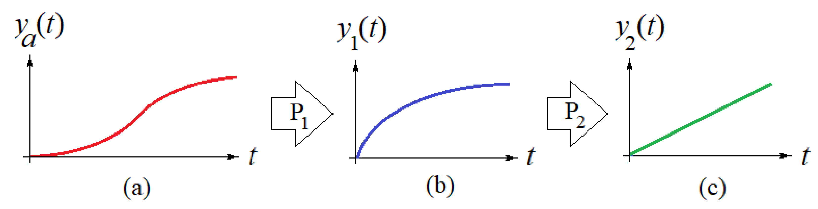
Figure 1 describes, pictorially, the steps taken to construct the model. Figure 1a depicts the shape of the curve (sigmoid) of the actual reported data, , which is the cumulative number of deceased people as a function of elapsed time, in days, since the outbreak of the pandemic for a specific country. Figure 1b depicts the natural logarithm of the actual recorded data obtained by a process P1, such as , and Figure 1c depicts the linearization of the curve in Figure 1b, i.e., , obtained by a linearization process P2.
The curves shown in Figure 1 are mathematical idealizations. These curves are actually described by the discrete daily values, which exhibit daily variations around these mathematically idealized curves or functions. To obtain the idealized curves, the data in the linearized curve in Figure 1c is approximated, using a weighted least squares fitting process, using a line equation, and then, the inverse processes and are applied successively to obtain the idealized first-order model (curve in Figure 1b), and the “actual” function (Figure 1a) that fits the actual recorded data.
Some key important information about the pandemic can be obtained from applying the processes shown in Figure 1, and by their corresponding inverse fitting processes:
- (1)
- An approximating function based on the proposed for the actual data that enables to predict near future outcomes and also enables to backtrack to estimate the initial values that might have been in those cases where the early or initial data on the pandemic outbreak is not available or was not reported or recorded.
- (2)
- A time-constant of the first order system that determines the time for which the number of deceased people will reach a particular percentage of the peak value. Recall that the response of a first-order system would reach a plateau value asymptotically. For example, the population will reach 99.33% of the plateau (or saturation) value for a period of time equal to five time constants or ; 99.75% of for , etc.
- (3)
- The asymptote’s (maximum) value that corresponds to the maximum number of people that would be deceased in the long run or for a long period of time.
- (4)
- The inflection point of the estimated curve at which the sigmoid changes concavity in Figure 1a. This point corresponds also to the time for which the maximum rate of deaths per day (i.e., ) occur.
We next describe the two processes P1 and P2 that convert the actual reported data of Figure 1a into that in Figure 1b (our model), and that in Figure 1b into the linear form in Figure 1c, respectively.
Process P1: This is a straightforward process that consists simply in taking the natural logarithm of the actual reported data and creating a new array with the natural logarithm of the actual data values versus time. That is, one generates the array of values
Since this data resembles the response of a first order-system to a Heaviside (or step) input function or stepwise excitation given by , where is the horizontal asymptote or saturation value, the curve in Figure 1c is given by
where the unit-step or Heaviside function is defined piecewise as .
In (2), t represents time in units of [day], is a growth rate in units of [1/day], and its reciprocal (days), the time-constant corresponding to the first order-process or system with initial condition This implies that which requires that This indicates that our coordinates require to start at the point where the first death occurs, that is, our first point is Therefore, the time t elapsed is measured from the day the first death occurred.
Process P2: This process linearizes the first order response curve, by transforming Equation (2) by means of a simple algebraic manipulation and a change of variables as follows: For , one has
Letting
one can obtain the linear equation , after determining via least squares process, which as shown in Figure 1c.
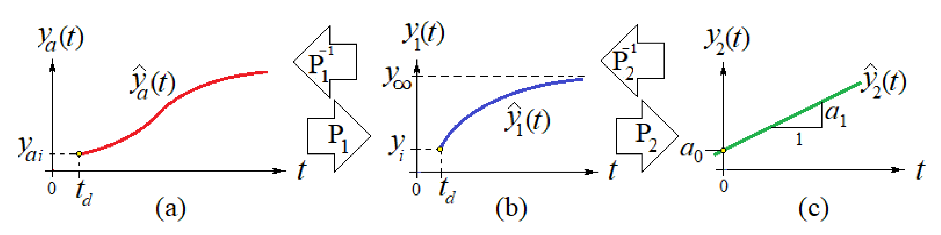
A more general model (3-parameters: , where is the asymptote value, is the shape parameter, and is a time delay) for a first order process response would include an initial value , where is a time-delay parameter of the process relative to some zero time reference and where the first data point exists, at The shifted version of the first order model shown in Figure 2b can be written in a more general form as
This function is essentially the response of a first-order system to a Heaviside [or step u(t)] input function. Derivation of this response is explained in the Supplementary Materials section, under Mathematics of first-order differential equation. Since this system is linear-time-invariant (LTI), any input delayed in time would correspond to the same delayed response. That is, one gets the response of a non-anticipative, causal system. More detailed description of LTI systems is given in reference [20].
The linearization (process P2) for this more general model is obtained algebraically as follows: From (5), for , one has
In (6), the time is a time shifted time. Letting
one can obtain a linear least-squares approximation equation shown in Figure 2c, where .
The right pointing arrows in Figure 2 indicate the two processes that transform the actual data into the curve corresponding to our model and the linearization of the data, while the left pointing arrows indicate the inverse processes, after the linearized data has been fitted via a weighted least Squares process.
After the coefficient estimate and of the line equation have been determined via a weighted least squares process, then the inverse processes and are applied to obtain the approximating or fitting functions and , respectively. A description of the inverse processes follows.
From (7), after the line coefficients have been determined via weighted least squares, one can write
Exponentiating both sides of the second equality in (8) and solving for yields
In (9) the values have been replaced back, and is the initial value . Once the function has been determined, then is obtained, simply, as
We note that in this study we use weighted least squares, where the weights get larger towards the later data and smaller towards the initial data values. The hypothesis here is that the residuals of the natural logarithm of the data and the fitting function become smaller as the rate of increase becomes smaller, towards the horizontal asymptote, so we weight heavier towards the region of smaller residuals. We tried several simple weighing functions that minimize the sum of squares of the residuals between the actual and the fitted data, such a linear, quadratic, and higher degree weighting functions, where the sum of the weights in each case is normalized to one. That is,
Linear weighting function: For meeting requirement given by Equation (11), the linear weights, as a function of the data point, are given by
Quadratic weighting function: For meeting requirement given by Equation (11), the quadratic weights, as a function of the data point, are given by
Cubic weighting function: For meeting requirement given by Equation (11), the cubic weights, as a function of the data point, are given by
Since all weights are positive, the weighted linear least squares parameter estimates
and are obtained by solving the normal equations, that is,
In (15), W is the diagonal matrix:
In (15), is the vector of coefficients, is the linear system matrix, and is the vector of transformed (linearized) values obtained via (4).
We note that the value for is obtained by a least squares approach as well, by minimizing the square of the residuals , that is, by finding a value that minimizes RSS = rTr where r is a column vector of the residuals and T denotes transposition. Additional details on the fitting process such as error estimates for the parameters and the corresponding sensitivities are provided in Appendix A.
2.2. Death Rates
The death rate in number of deaths per day is calculated by taking the derivative of the estimated actual accumulated death data computed by (10). Taking the time derivative of (10) yields
In (17), the time derivative of is obtained from (9) as
The graph of (17) shows an initial gradual increase in the values of the rate or time derivative in units of [deaths/day], then it reaches a peak or maximum value corresponding to the inflection point of the sigmoid and after this point commences to decrease towards the value of zero, asymptotically. The graphs of the death rates are also given for each of the selected countries in the Supplementary Materials section and for Germany in Figure 3 in the Results section. These rate graphs are useful to find the time when the peak rate occurs, date from which the effects of pandemic begin to diminish.
3. Results
The model was applied to the actual data that was collected on a daily basis from the web site given in reference [11] which provides historical and daily updated values of the COVID-19 infections and presumed deaths for numerous countries. Initially, we collected the data for a limited set of countries, those that were reported initially, starting with China. The number of countries that were included in our data set increased in time as the pandemic spread over the world. In Section 3.1, our proposed First Order model is fitted to each of the countries on the initial data set. In Section 3.2, already published models are fitted to this data set, and the results are compared to those in our proposed first order model.
3.1. Simulation Results
The data we collected for this article span from 21 January 2020 (earliest data for China) to 31 May 2020, which we considered sufficient, in number of data points, to test our model within varying intervals of time for verifying the model estimates and the characterization of the model parameters with the values of the reported data [11].
Daily data records for ten of the countries utilized in the simulations are given in Table S1 in the Supplementary Materials section. The graphs corresponding to the actual data and the estimated model data [ and ; and ; and ]; the horizontal asymptote value ; and the Process-P1 time constant [days] for the curve for each country listed in Table S1 are also illustrated in the Supplementary Materials section. A fraction (start and end) of Table S1 is repeated here just for reference in Table 1:
The graphs that were generated for several of the countries listed in Table S1 of the Supplementary Materials section include the following graphs:
- (1)
- Actual data and the actual data model estimates curve .
- (2)
- The natural logarithm of the actual data and the model estimate curve .
- (3)
- The linearization of the actual data logarithm and the linear fit .
- (4)
- The derivative of the actual data model .
- (5)
- Additional graphs of interest, like fit residuals n some of the cases analyzed.
The numerical computations were performed using MATLAB (from MathWorks) scripts written by the authors, which included some high-level (canned-in) commands. A Summary of modeling results/parameters, for the given data recorded in Table 1 for the ten countries selected are provided in Table 2. Very good fits of the proposed First Order model with a RSS value below one were obtained for CN, SK, and the US; good fits with an RSS value between one and two were obtained for IT, IR, SP, DE, UK, and NE. The worst fit was obtained with an RSS value larger than 2 for FR.
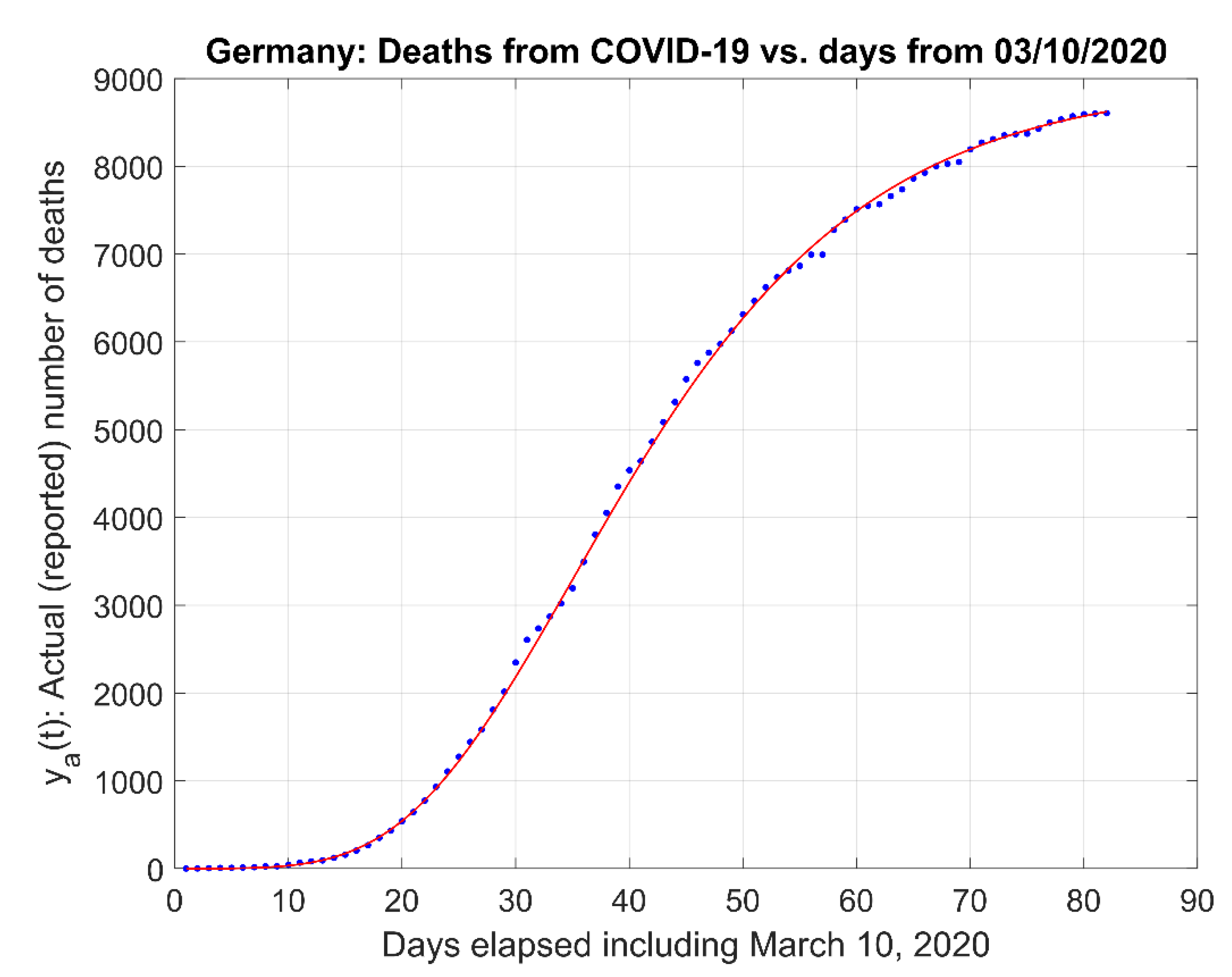
For completeness, we provide below a sample of the modeling process for the data corresponding to Germany (DE), corresponding to Figure 4, Figure 5 and Figure 6. For the remaining countries, similar figures are reported in the Supplementary Materials section.
3.2. Comparison to Other Models
Other log(N) models besides the model presented here, which we call First-Order model given by
where
are presented and compared next. The model comparison graphs and the modified forms of these models are also described in Appendix B. These models have been widely applied (and compared) for a diversity of population growth phenomena. The following models are reported in [12,17], and [21] and include:
Gompertz model which is a three-parameters curve
Richards model which is a four-parameters curve
Logistic model, which is another three-parameter curve
Stannard model, which is a four-parameter curve
and Schnute model another four-parameters curve
Parameters like a, b, c, ν, τ, k, l, p, y1, τ1, and τ2 in these models denote shape, shift, and/or scale parameters (see first column in Table 3).
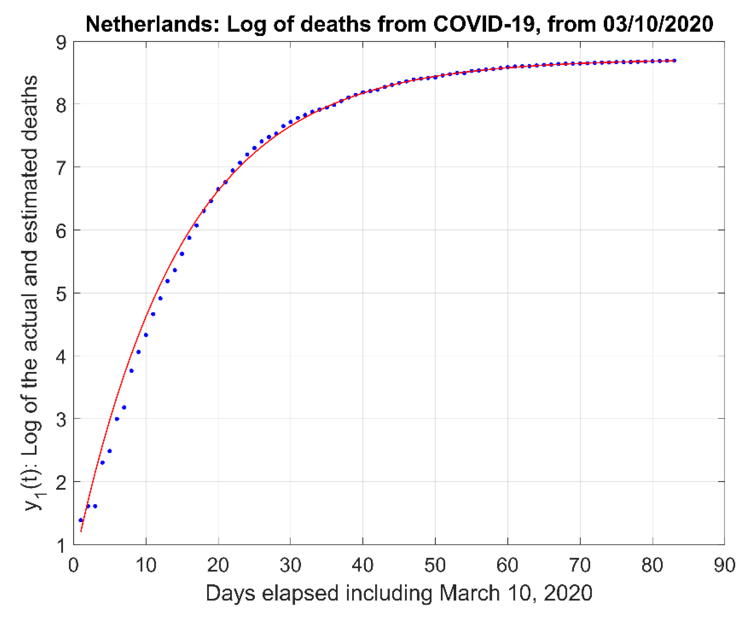
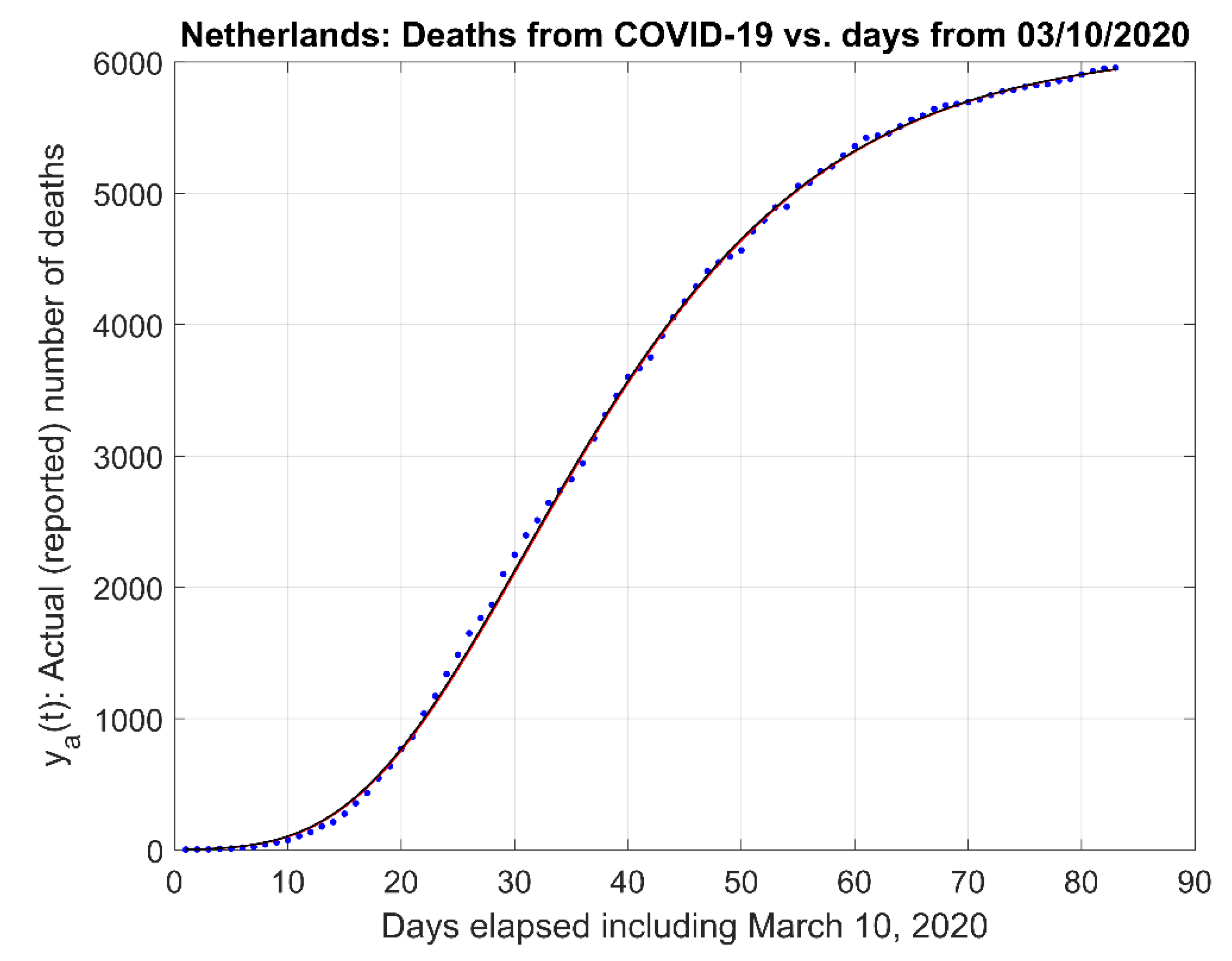
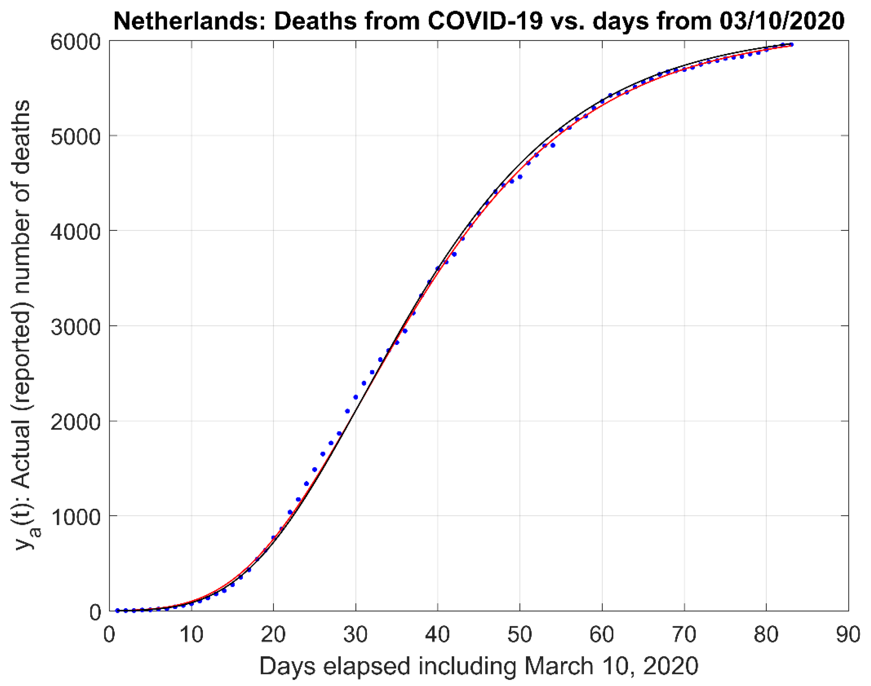
These five models, (21) to (25) and the proposed First-Order model, (19) and (20) were next compared to each other using the logarithm of the original data, , for the Netherlands. Figure 7 depicts the corresponding First-Order model fit (solid red line) to the data (blue dots).
.
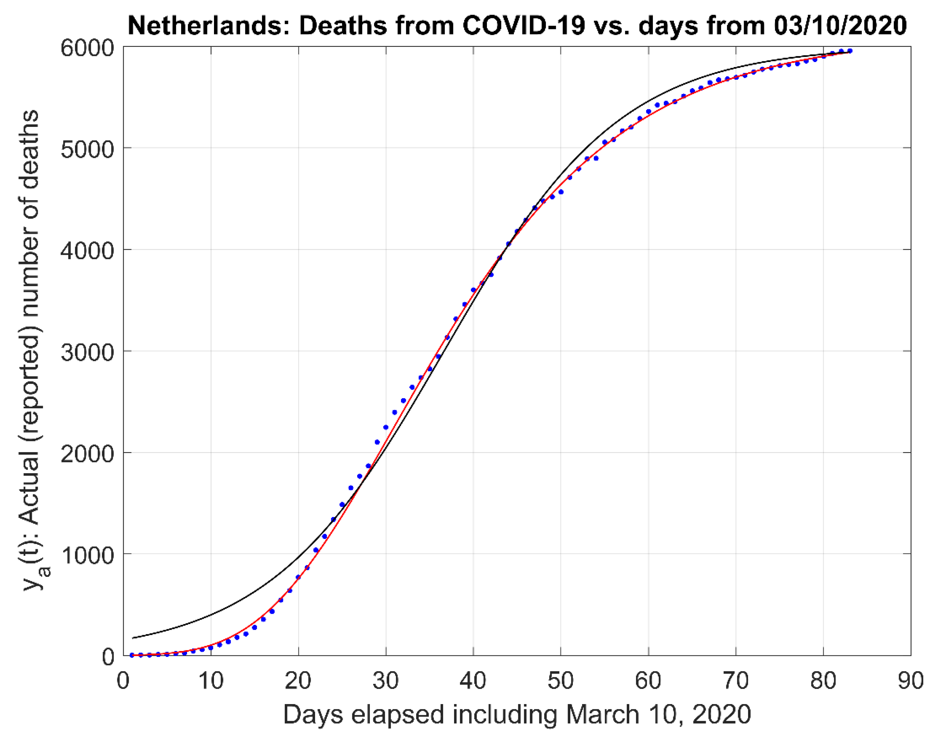
A comparison between the proposed First-Order model (19) and (20), and the Gompertz model (21), using the following linearization for the Gompertz model
shows a close agreement as depicted in Figure 8. Comparisons between the proposed First-Order model and the other models, Richards, Logistic, Stannard, and Schnute, are shown in Appendix B. Table 3 summarizes the results for these comparisons by reporting the residuals obtained between the natural logarithms of the actual data and the natural logarithms of each model’s fitted data. These parameters were obtained via weighted linear least squares, when linearization of the models was possible, and via nonlinear least-squares methods, when linearization was not possible, which included modified Gauss–Newton, and Nelder–Mead (downhill simplex method) techniques and other appropriate methods for the minimization of the objective function, the sum of squares of the residuals or errors between the actual and fitted (or estimated) data. The lower the reported residuals mean value and/or the residuals RSS value, the better the fit.
We find from the comparisons with other log(N)-type models that our model results are in very close agreement and that resulting curves are almost indistinguishable in the graphical rendering of these pair-wise comparisons between our model and the other models utilized, including those with larger number of parameters, as depicted in the graphs in Figure 8 and in those in Appendix B.
Other models such as in reference [10] were also studied but not compared, as we concentrated in the log(N) based ones.
4. Discussion
The model presented here is meant to be a simple one that can be applied to infectious diseases and other biological growth phenomena that follow a sigmoidal behavior. The list of models that have been developed and/or put to use in practice triggered by the COVID19 pandemic is widely varied in their underlying mathematical approach, using statistical, biological-based, dynamical systems, time-series analysis, and others. The Center for Disease Control and Prevention (CDC) [22] receives forecasts from several contributors that include Universities, Research Groups, Defense, and Private Corporations (Google, Walmart, etc.) that provide both National and State predictions for a forecast interval of 4 weeks, for both new and total presumed deaths, and provides an ensemble forecast at the National and State level, based on those provided by 35 modeling groups. In [22] there is a link with information on, and links to, the various models [23]. Another link [24] provides predictions or forecasts comparisons between the model for the US and States, which are very comparable in their 4 weeks forecasts. One model the authors considered of interest was the one developed by the Discrete Dynamical Systems (DDS) group [25] based on statistics and on discrete linear dynamical systems (LDS) theory. Even though the complexity of the models described are quite varied, it is interesting to note key pros and cons factors on each, as described by the New England Journal of Medicine on their article [26] on epidemiological models: “Wrong but Useful—What COVID-19 Epidemiologic Models can and cannot tell us”.
5. Conclusions
In this paper, we derived and compared a simple model for estimating the evolution of a disease and other biological growth processes that follow, as it occurs in many cases, a natural sigmoidal evolutionary response. Models can obviously be improved or expanded to accommodate any particular systemic bias or model variations in the data that is collected, but complexity comes at the cost of less robustness in the predictions, or higher parameter sensitivities (partial derivatives) unless a dynamical model is employed that continually updates the model parameters as new data is considered that follow latest data trends, or that incorporates a fading memory of earlier collected data. These dynamical models can be designed based on time-series analysis that includes forecasting and control theory and stochastic processes models. While the set of possibilities in creating models for estimation, prediction, or forecasting is quite large, it is always convenient to have a simple model or a set of proven simple models as a basis for building more complex ones.
Supplementary Materials
The following are available online at https://0-www-mdpi-com.brum.beds.ac.uk/2078-1547/12/1/3/s1. Figure S1: reported data of accumulated presumed deaths due to COVID-19 for China (CN) with discontinuities; Figures S31–S34 corresponding Figure 3, Figure 4, Figure 5 and Figure 6 of the main manuscript; and Figure S40 for the Netherlands (NE) corresponding to Figure 7 of the main manuscript. The remaining figures in the Supplementary Materials section for the ten selected countries are similar, except for Figure S20, the graph of the residuals of the fit for the USA (US). Table S1: this entire data set is utilized, which depicts the accumulated number of presumed deaths due to COVID-19 for all ten countries over a given time span. Additionally, the Supplementary Materials provides a brief review of the Mathematics of first-order differential equation.
Author Contributions
Conceptualization, R.A.G.U.; formal analysis, R.A.G.U. and K.S.; funding acquisition, R.A.G.U. and K.S.; investigation, R.A.G.U. and K.S.; methodology, R.A.G.U.; supervision, K.S.; visualization, R.A.G.U.; writing—original draft, R.A.G.U.; writing—review and editing, R.A.G.U. and K.S. All authors have read and agreed to the published version of the manuscript.
Funding
This work was supported by the University of Colorado, Colorado Springs (UCCS) Center for the University of Colorado BioFrontiers Institute and by the UCCS Graduate Research and Professional Development Award.
Data Availability Statement
Publicly available datasets were analyzed in this study. This data can be found in: https://www.worldometers.info/coronavirus/.
Conflicts of Interest
The authors declare no conflict of interest.
Appendix A
Details on the Least-Square Model Parameter Estimates
The sample figure (Figure 5 for (DE)) provided in Section 3 (3. Results) depicts the linearized model data and the weighted least squares linear fit applied to this data. This fitting process can also be represented as a chi-square fitting process, basically a weighted least squares fitting process. The following is described in [27], which we follow next, where the objective is to minimize the function
In (A1), the set of (model) parameters, are adjusted to minimize the value of , where m is the number of parameters the particular model utilizes; the sub-index i represents the data point number; denotes the ith actual measurements or the y-value of the given ith data point; and is the ith model fit value (in our case the ith linear fit estimate, (denoted with the caret symbol “^”); and is the standard deviation associated with ith measurement or recorded data, where normal-distribution is assumed. According to [27], the sum in (A1) of N-squares of normally distributed quantities, each normalized to unit variance are not statistically independent, and the probability distribution (pdf) for different values of at its minimum can be derived analytically. This is the chi-square distribution for N-m degrees of freedom. From here, a probabilistic approach is utilized to infer a goodness of fit. Data can be generated to test the model adequacy (e.g., via Monte-Carlo simulations). Since the uncertainties are associated when the measurements are not initially known, then we assume a priori some standard deviation common to all of the measurement points, say, which are associated to our weighting functions estimates described previously, and assume that the model fits well. Considerations related to the fitting are utilized to derive the a posteriori value for . Therefore, initially, we assume a value for our weights, then fit the model parameters by minimizing , and finally recomputing
When the measurement error is not known (in our case the error for reported numbers), this method provides some error-bar to be assigned to the points. Taking the derivative of (A1) with respect to the parameters , we obtain equations that must hold for the minimum:
For the case of fitting the data to a straight line (as is our case here), the approach just described follows:
Consider the problem of fitting a set of N data points to the straight-line model
We assume that the uncertainty associated with each measurement is known, and that is known exactly. To measure how well the model agrees with the data, we apply the chi-square merit Function (A1), which for this case is
For determining the parameters that minimize this function, we apply the usual rules from calculus:
Letting
we can write the system (A6) as
Solving this (simple) system of equations (e.g., via Cramer’s rule) yields
Next, we need to determine the uncertainties in the parameters a and b. Considering propagation of errors, the variance in the value of any function f will be
For the straight line, the derivatives of a and b with respect to can be directly evaluated from their solutions (A9):
Summing over the points we get
Appendix B
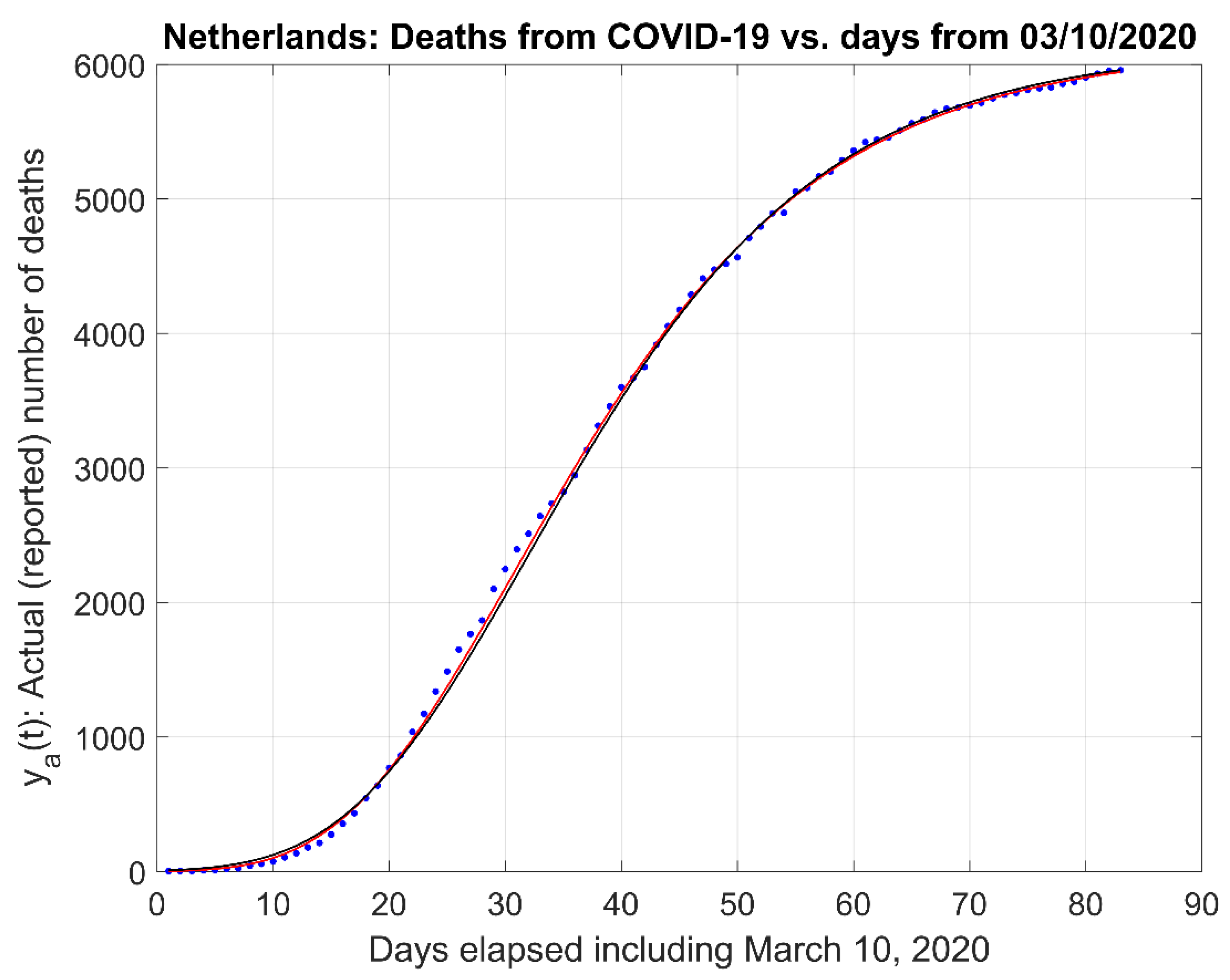
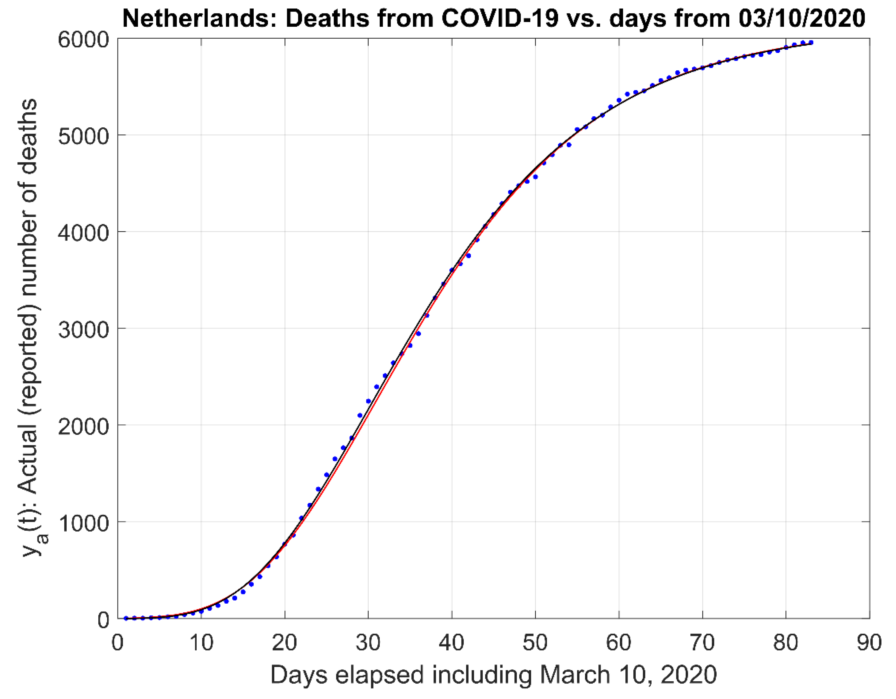
This Appendix depicts the comparisons of our proposed First Order Model to the Richards, Logistic, Stannard, and Schnute models, illustrated in Figure A1, Figure A2, Figure A3 and Figure A4, respectively, and the modified forms of the equations are described in Equations (A13)–(A16). This Appendix B complements the information provided in the Section 3.2, Comparison to other Models.
Figure A1.
Comparison of the First-Order model and Richards model. (Red trace is First Order; Black trace is Richards).
Figure A1.
Comparison of the First-Order model and Richards model. (Red trace is First Order; Black trace is Richards).

Figure A2.
Comparison of the First-Order model and Logistic model. (Red trace is First Order; Black trace is Logistic).
Figure A2.
Comparison of the First-Order model and Logistic model. (Red trace is First Order; Black trace is Logistic).

Figure A3.
Comparison of the First-Order model and Stannard model. (Red trace is First Order; Black trace is Stannard).
Figure A3.
Comparison of the First-Order model and Stannard model. (Red trace is First Order; Black trace is Stannard).

Figure A4.
Comparison of the First-Order model and Schnute model. (Red trace is First Order; Black trace is Schnute).
Figure A4.
Comparison of the First-Order model and Schnute model. (Red trace is First Order; Black trace is Schnute).

There are also modified forms of the Logistic, Gompertz, Richards, and Schnute models from reference [12,17,21], whose simpler forms were discussed in Section 3.2. Comparisons to other models are listed below for completeness. The parameter is the slope of the tangent line at the inflection point of the sigmoid (at t = ti), i.e., the maximum derivative value of the sigmoid.
Logistic—Modified Form:
Gompertz—Modified Form:
Richards—Modified Form:
Schnute—Modified Form:
References
- Anderson, R.M.; Anderson, B.; May, R.M. Infectious Diseases of Humans: Dynamics and Control; Oxford University Press: Oxford, UK, 1992. [Google Scholar]
- Nowak, M.A.; May, R. Virus Dynamics: Mathematical Principles of Immunology and Virology; Oxford University Press: Oxford, UK, 2000. [Google Scholar]
- Adiga, A.; Dubhashi, D.; Lewis, B.; Marathe, M.; Venkatramanan, S.; Vullikanti, A. Mathematical Models for COVID-19 Pandemic: A Comparative Analysis. J. Indian Inst. Sci. 2020, 100, 793–807. [Google Scholar] [CrossRef] [PubMed]
- Giordano, G.; Blanchini, F.; Bruno, R.; Colaneri, P.; di Filippo, A.; di Matteo, A.; Colaneri, M. Modelling the COVID-19 Epidemic and Implementation of Population-Wide Interventions in Italy. Nat. Med. 2020, 26, 855–860. [Google Scholar] [CrossRef] [PubMed]
- Oliveira, J.F.; Jorge, D.C.P.; Veiga, R.V.; Rodrigues, M.S.; Torquato, M.F.; da Silva, N.B.; Fiaccone, R.L.; Cardim, L.L.; Pereira, F.A.C.; de Castro, C.P.; et al. Mathematical Modeling of COVID-19 in 14.8 Million Individuals in Bahia, Brazil. Nat. Commun. 2021, 12, 333. [Google Scholar] [CrossRef] [PubMed]
- Baek, Y.J.; Lee, T.; Cho, Y.; Hyun, J.H.; Kim, M.H.; Sohn, Y.; Kim, J.H.; Ahn, J.Y.; Jeong, S.J.; Ku, N.S.; et al. A Mathematical Model of COVID-19 Transmission in a Tertiary Hospital and Assessment of the Effects of Different Intervention Strategies. PLoS ONE 2020, 15, e0241169. [Google Scholar] [CrossRef] [PubMed]
- Tiwari, V.; Deyal, N.; Bisht, N.S. Mathematical Modeling Based Study and Prediction of COVID-19 Epidemic Dissemination Under the Impact of Lockdown in India. Front. Phys. 2020, 8, 586899. [Google Scholar] [CrossRef]
- Kyrychko, Y.N.; Blyuss, K.B.; Brovchenko, I. Mathematical Modelling of the Dynamics and Containment of COVID-19 in Ukraine. Sci. Rep. 2020, 10, 1–11. [Google Scholar] [CrossRef] [PubMed]
- Iboi, E.; Sharomi, O.O.; Ngonghala, C.; Gumel, A.B. Mathematical Modeling and Analysis of COVID-19 Pandemic in Nigeria. Math. Biosci. Eng. 2020, 17, 7192–7220. [Google Scholar] [CrossRef] [PubMed]
- Cherniha, R.; Davydovych, V. A Mathematical Model for the COVID-19 Outbreak and Its Applications. Symmetry 2020, 12, 990. [Google Scholar] [CrossRef]
- COVID-19 Coronavirus Pandemic|Worldometer. Available online: https://www.worldometers.info/coronavirus/ (accessed on 27 October 2020).
- Zwietering, M.H.; Jongenburger, I.; Rombouts, F.M.; van’t Riet, K. Modeling of the Bacterial Growth Curve. Appl. Environ. Microbiol. 1990, 56, 1875–1881. [Google Scholar] [CrossRef] [PubMed] [Green Version]
- Strogatz, S.H. Nonlinear Dynamics and Chaos: With Applications to Physics, Biology, Chemistry, and Engineering; Addison Wesley: Boston, MA, USA, 1994. [Google Scholar]
- Brauer, F.; van den Driessche, P.; Wu, J. Mathematical Epidemiology (Lecture Notes in Mathematics); Springer: Berlin/Heidelberg, Germany, 2008. [Google Scholar]
- Sperschneider, V. Bioinformatics: Problem Solving Paradigms; Springer: Berlin/Heidelberg, Germany, 2008. [Google Scholar]
- Iglesias, P.A.; Ingalls, B.P. Control. Theory and Systems Biology; The MIT Press: Cambridge, MA, USA, 2010. [Google Scholar]
- Nowak, M.A. Evolutionary Dynamics: Exploring the Equations of Life; The Belknap Press of Harvard University Press: Cambridge, MA, USA, 1994. [Google Scholar]
- Bohner, M.; Streipert, S.; Torres, D.F.M. Exact Solution to a Dynamic SIR Model. Nonlinear Anal. Hybrid. Syst. 2018, 32, 228–238. [Google Scholar] [CrossRef] [Green Version]
- Murray, C.J. Forecasting the Impact of the First Wave of the COVID-19 Pandemic on Hospital Demand and Deaths for the USA and European Economic Area Countries. medRxiv 2020. [Google Scholar] [CrossRef] [Green Version]
- Phillips, C.; Parr, J.; Riskin, E. Signals, Systems, & Transforms; Pearson Education Limited: London, UK, 2014. [Google Scholar]
- da Silva, A.P.R.; Longhi, D.A.; Dalcanton, F.; de Aragão, G.M.F. Modelling the Growth of Lactic Acid Bacteria at Different Temperatures. Braz. Arch. Biol. Technol. 2018, 61, 18160159. [Google Scholar] [CrossRef]
- COVID-19 Forecasts: Deaths | CDC. Available online: https://www.cdc.gov/coronavirus/2019-ncov/covid-data/forecasting-us.html (accessed on 27 October 2020).
- COVID-19-Forecasts/GitHub. Available online: https://github.com/cdcepi/COVID-19-Forecasts/blob/6768f5dbc09dd03833584f9f2dc156c157b2247f/COVID-19_Forecast_Model_Descriptions.md (accessed on 30 October 2020).
- COVID 19 Forecast Hub. Available online: https://covid19forecasthub.org/ (accessed on 27 October 2020).
- Kalantari, R.; Zhou, M. Graph Gamma Process Generalized Linear Dynamical Systems. arXiv 2020, arXiv:2007.12852. [Google Scholar]
- Holmdahl, I.; Buckee, C. Wrong but Useful—What Covid-19 Epidemiologic Models Can and Cannot Tell Us. N. Engl. J. Med. 2020, 383, 303–305. [Google Scholar] [CrossRef] [PubMed]
- Press, W.H.; Flannery, B.P.; Teukolsky, S.A.; Vetterling, W.T. Numerical Recipes in C: The Art of Scientific Computing; Cambridge University Press: Cambridge, UK, 1988. [Google Scholar]
Figure 1.
(a) Actual sigmoidal curve. (b) Logarithm of the sigmoidal curve. (c) Linearization of the logarithm of the sigmoidal curve in (a).
Figure 1.
(a) Actual sigmoidal curve. (b) Logarithm of the sigmoidal curve. (c) Linearization of the logarithm of the sigmoidal curve in (a).

Figure 2.
A more general model: (a) Actual recorded data and its approximating function . (b) Logarithm of the sigmoidal curve and its approximating function . (c) Linearization of the curve and its approximating function .
Figure 2.
A more general model: (a) Actual recorded data and its approximating function . (b) Logarithm of the sigmoidal curve and its approximating function . (c) Linearization of the curve and its approximating function .

Figure 3.
Actual and modeled number of presumed deaths using only data from 10 March 2020 for Germany.
Figure 3.
Actual and modeled number of presumed deaths using only data from 10 March 2020 for Germany.

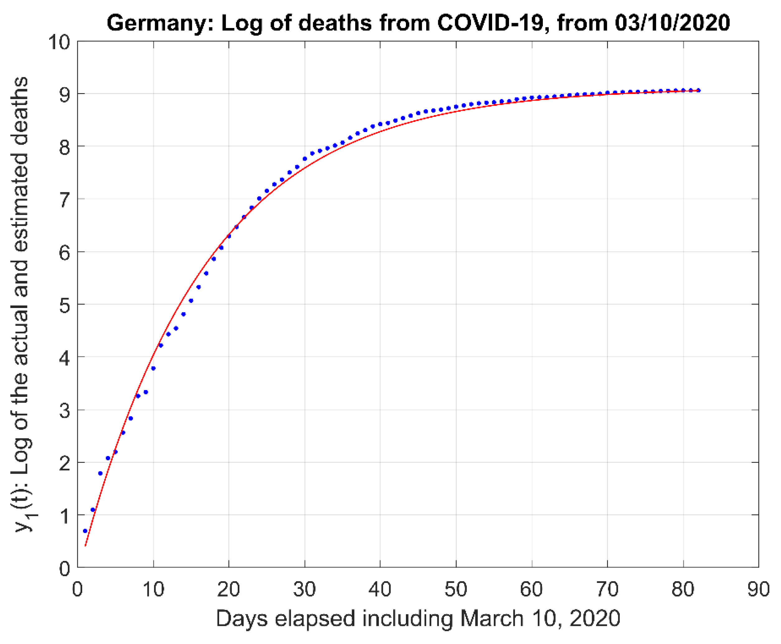
Figure 4.
Natural logarithm of the actual (and extrapolated) data in Figure 3. We note in this figure the plateau or saturation value is , and the time-constant is days. These numbers indicate that the number of deaths might reach a value of people. The sum of squares of the residuals (i.e., or estimated minus actual values) for this data is RSS = rTr = 1.2356.

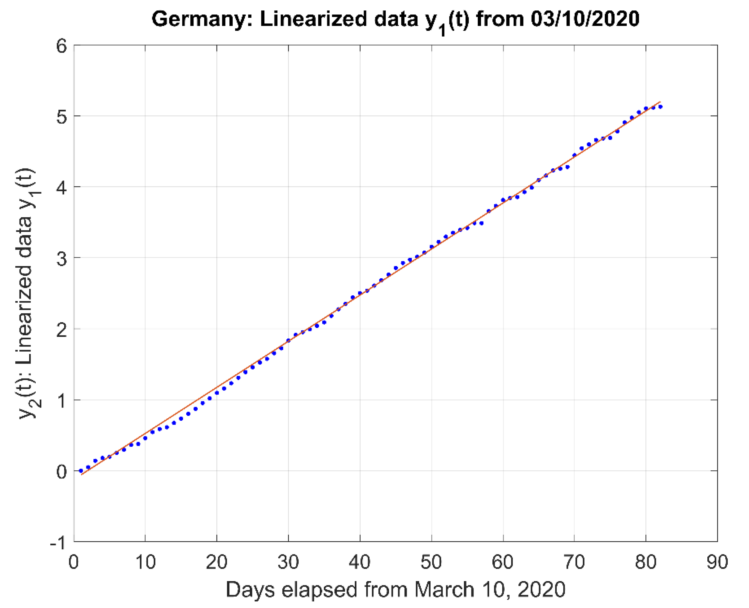
Figure 5.
Linearization of data in Figure 4 (dots) and Weighted Least Squares Linear Fit (continuous curve).
Figure 5.
Linearization of data in Figure 4 (dots) and Weighted Least Squares Linear Fit (continuous curve).

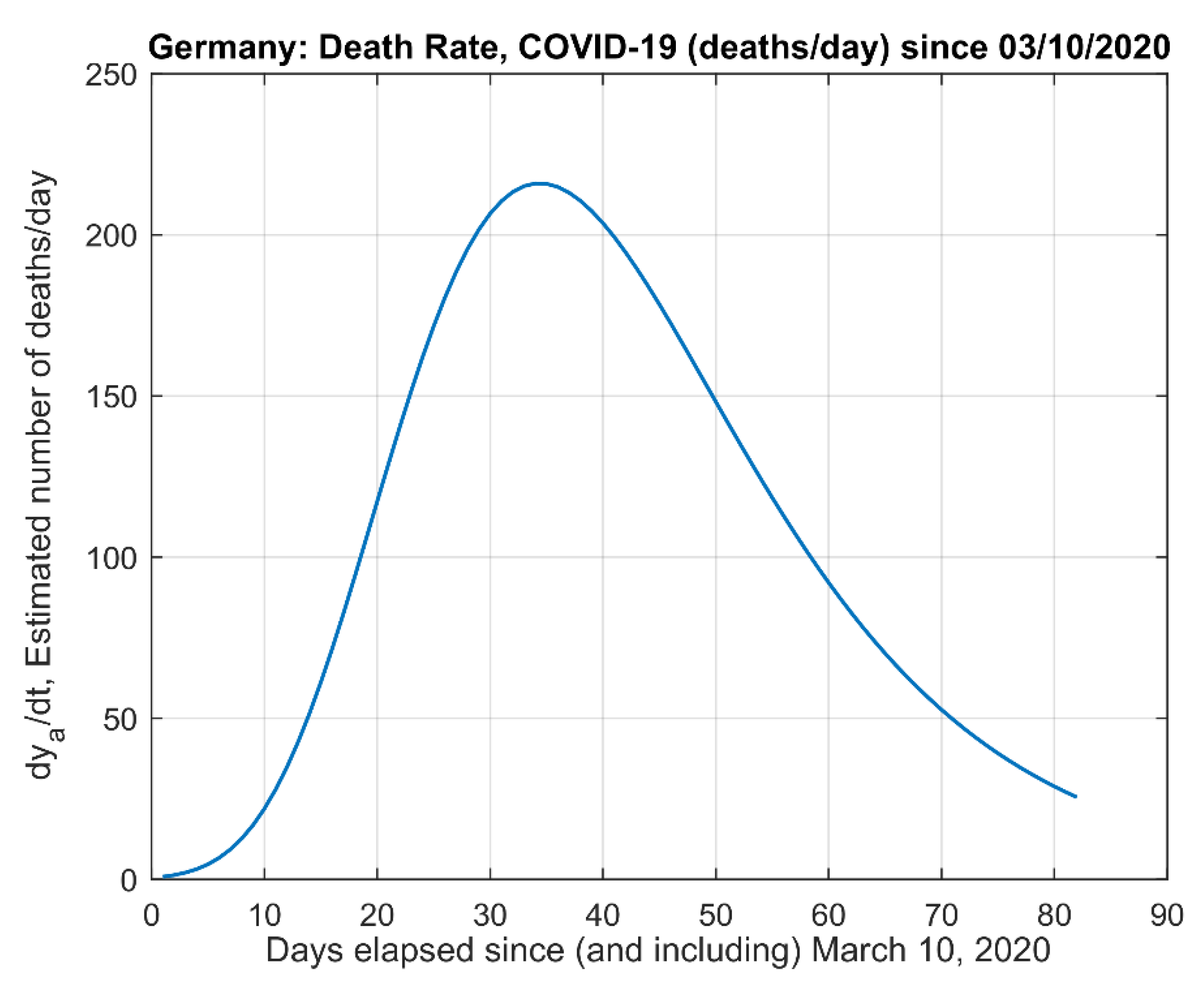
Figure 6.
Data-Rate corresponding to the derivative of the estimated data in Figure 3. The peak value occurred on 13 April 2020, according to the model.
Figure 6.
Data-Rate corresponding to the derivative of the estimated data in Figure 3. The peak value occurred on 13 April 2020, according to the model.

Figure 7.
First-order model fit (red solid line) for Netherlands, where

Figure 8.
Comparison of the First-Order model and Gompertz model. (Red trace is First-Order, Black trace is Gompertz, Dots are original data).
Figure 8.
Comparison of the First-Order model and Gompertz model. (Red trace is First-Order, Black trace is Gompertz, Dots are original data).


Table 1.
Accumulated number of presumed deaths due to COVID-19. Abbreviation Key: China (CN), South Korea (SK), Italy (IT), Iran (IR), USA (US), Spain (SP), Germany (DE), United Kingdom (UK), Netherlands (NE).
Table 1.
Accumulated number of presumed deaths due to COVID-19. Abbreviation Key: China (CN), South Korea (SK), Italy (IT), Iran (IR), USA (US), Spain (SP), Germany (DE), United Kingdom (UK), Netherlands (NE).
| Date | CN | SK | IT | IR | US | SP | FR | DE | UK | NE |
|---|---|---|---|---|---|---|---|---|---|---|
| 01/21 | 9 | 0 | 0 | 0 | 0 | 0 | 0 | 0 | 0 | 0 |
| 01/22 | 17 | 0 | 0 | 0 | 0 | 0 | 0 | 0 | 0 | 0 |
| 01/23 | 25 | 0 | 0 | 0 | 0 | 0 | 0 | 0 | 0 | 0 |
| … | ||||||||||
| 05/29 | 4634 | 269 | 33,229 | 7677 | 104,542 | 27,121 | 28,714 | 8594 | 38,593 | 5931 |
| 05/30 | 4634 | 269 | 33,340 | 7734 | 105,557 | 27,125 | 28,771 | 8600 | 38,819 | 5951 |
| 05/31 | 4634 | 270 | 33,415 | 7797 | 106,195 | 27,127 | 28,802 | 8605 | 38,934 | 5956 |
| Date | CN | SK | IT | IR | US | SP | FR | DE | UK | NE |
Table 2.
Comparison of key model parameters for the countries listed. N is number of people. Abbreviation Key: China (CN), South Korea (SK), Italy (IT), Iran (IR), USA (US), Spain (SP), Germany (DE), United Kingdom (UK), Netherlands (NE).
Table 2.
Comparison of key model parameters for the countries listed. N is number of people. Abbreviation Key: China (CN), South Korea (SK), Italy (IT), Iran (IR), USA (US), Spain (SP), Germany (DE), United Kingdom (UK), Netherlands (NE).
| Parameter Country | RSS | ||||
|---|---|---|---|---|---|
| CN | 8.4480 | 4664 | 14.15 | 0.39 | 0.4399 |
| SK | 5.6173 | 275 | 19.42 | 0.06 | 0.5745 |
| IT | 10.4574 | 34,801 | 18.00 | 1.26 | 1.4644 |
| IR | 9.0025 | 8124 | 20.53 | 1.39 | 1.0933 |
| US | 11.6622 | 116,099 | 17.13 | 1.10 | 0.3230 |
| SP | 10.2858 | 29,315 | 14.04 | 1.38 | 1.1376 |
| FR | 10.3182 | 30,279 | 17.89 | 1.93 | 2.2950 |
| DE | 9.1235 | 9168 | 16.70 | 1.57 | 1.2356 |
| UK | 10.6360 | 41,606 | 17.16 | 2.28 | 1.2653 |
| NE | 8.720 | 6124 | 14.85 | 1.37 | 1.2483 |
Table 3.
Model Comparisons for Netherlands Data with y2 = 6124. The Statistics values here correspond to the residuals obtained between the natural logarithms of the actual data and the natural logarithms of each model’s fitted data.
Table 3.
Model Comparisons for Netherlands Data with y2 = 6124. The Statistics values here correspond to the residuals obtained between the natural logarithms of the actual data and the natural logarithms of each model’s fitted data.
| Model/Parameters | Residuals Mean Value | Residuals RSS |
|---|---|---|
| First-Order α = 0.0674; td = 1.37 | 0.0414 | 1.2483 |
| Gompertz b = 2.0755; c = −0.0674 | 0.0541 | 1.3919 |
| Richards ν = 0.01; τ = 31; k = 0.07 | 0.0057 | 0.8451 |
| Logistic b = 3.65; c = 0.099 | 86.6 | 1.53 × 10² |
| Stannard k = 0.74; l = 1.0; p = 10.50 | 0.1102 | 1.4161 |
| Schnute a = 0.0655; b = 0.055; y1 = 7.274; τ1 = 3.79; τ2 = 138 | 0.0179 | 1.8290 |
Publisher’s Note: MDPI stays neutral with regard to jurisdictional claims in published maps and institutional affiliations. |
© 2021 by the authors. Licensee MDPI, Basel, Switzerland. This article is an open access article distributed under the terms and conditions of the Creative Commons Attribution (CC BY) license (http://creativecommons.org/licenses/by/4.0/).
Share and Cite
MDPI and ACS Style
Unglaub, R.A.G.; Spendier, K. A Model for the Spread of Infectious Diseases with Application to COVID-19. Challenges 2021, 12, 3. https://0-doi-org.brum.beds.ac.uk/10.3390/challe12010003
AMA Style
Unglaub RAG, Spendier K. A Model for the Spread of Infectious Diseases with Application to COVID-19. Challenges. 2021; 12(1):3. https://0-doi-org.brum.beds.ac.uk/10.3390/challe12010003
Chicago/Turabian StyleUnglaub, Ricardo A. G., and Kathrin Spendier. 2021. "A Model for the Spread of Infectious Diseases with Application to COVID-19" Challenges 12, no. 1: 3. https://0-doi-org.brum.beds.ac.uk/10.3390/challe12010003
Note that from the first issue of 2016, this journal uses article numbers instead of page numbers. See further details here.