The Temperature Forecast of Ship Propulsion Devices from Sensor Data

Abstract

The big data from various sensors installed on-board for monitoring the status of ship devices is very critical for improving the efficiency and safety of ship operations and reducing the cost of operation and maintenance. However, how to utilize these data is a key issue. The temperature change of the ship propulsion devices can often reflect whether the devices are faulty or not. Therefore, this paper aims to forecast the temperature of the ship propulsion devices by data-driven methods, where potential faults can be further identified automatically. The proposed forecasting process is composed of preprocessing, feature selection, and prediction, including an autoregressive distributed lag time series model (ARDL), stepwise regression (SR) model, neural network (NN) model, and deep neural network (DNN) model. Finally, the proposed forecasting process is applied on a naval ship, and the results show that the ARDL model has higher accuracy than the three other models.

1. Introduction

In recent years, with the increase of global trade volume, seaborne transport volume shows a momentum of accelerating rise, and maritime transport has undoubtedly become a very important transport mode. However, the problems brought about by the maritime industry in terms of marine environment and ecological protection, energy sustainability, etc., have become increasingly serious. It is imperative for ships to save energy, reduce emissions, and minimize marine pollution by means of using new and cleaner energy as ship power, building ships with new materials, economically efficient hull design, economic speed, and intelligent ship fault prediction.

The ship propulsion system [1] is the heart of ship, and it is the basic guarantee for the safety of the ship operation. Once the fault of propulsion devices occurs, it will not only affect the normal operation of the entire ship’s power plants, but also cause a series of environmental problems, such as diesel oil leakage and seawater pollution. With the continuous improvement of scale and automation of modern ship propulsion systems, the design of various control systems is more and more complex, which makes it difficult to locate and solve the faults in time. However, many propulsion devices of ships are equipped with sensors, and the temperature change of the ship’s propulsion devices can be forecasted for identifying potential faults, which will then save the cost of operation and maintenance, reduce energy consumption, and then ensure the sustainable development of ship energy.

There are many references focusing on the analysis of ship sensing data. For example, Onwuegbuchunam et al. [2] conducted research and analysis on the marine pollution of ships in Nigeria, and the integrated model was proposed as an alternative administrative tool for monitoring and controlling pollution in seaports. Iodice et al. [3] proposed a numerical approach to assess air pollution by ship engines in maneuver mode and fuel switch conditions, and it was also used to assess the impact of marine engine pollutant emissions on ambient air quality in coastal areas. Kim and Park [4] proposed a method to consider the optimization of the hull form of ULCS (Ultra Large Container Ship) in green ship design, and confirmed that the energy efficiency of the optimized hull form was improved by the proposed total energy formula. Gudehus and Kotzab [5] developed a model for the economic travel speed of container ships, which showed how the travel speed impacts the profit situation as well as the environmental sustainability. The above references focus on data-driven methods to solve ship problems, but they are not fault or prediction problems. Meanwhile, there are some references for predicting the possible fault locations and causes, and providing maintenance decisions and suggestions, so as to take effective measures to quickly troubleshoot. For instance, Feng and Li [6] aimed at the inaccurate and time-consuming problems of the fault diagnosis method for a large-scale ship engine, and proposed an intelligent diagnosis method for large-scale ship engine fault in a non-deterministic environment based on neural network. Tang et al. [7] proposed a fault diagnosis system of ship power plants based on a C/S (Client/Server) and B/S (Browser/Server) hybrid structure for the ship power plant fault diagnosis system, which provided a good solution for the development of intelligent ships. Yang and Tang [8] proposed a method for fault pattern recognition and state prediction of marine power plants based on HMM-SVR. The above research provides a lot of prior knowledge for ship condition prediction and fault diagnosis. However, the data collected by various sensors is time-series data, and it is necessary to maintain its time-series characteristics. So, we need to consider its time characteristics in the research process as follows: Wu et al. [9] proposed a hybrid model to represent the tracking dynamic behavior of ships in order to achieve ship-tracking control along the desired path at constant speed. McCullough et al. [10] proposed constructing ordinal networks from discrete sampled continuous chaotic time series, and then regenerated new time series by taking random walks on the ordinal networks. Cinar et al. [11] combined the time series with the recurrent neural network (RNN), and proposed the period-aware content attention RNNs for time series forecasting with missing values. Yang and Liu [12] proposed a time-series prediction model based on the hybrid combination of high-order FCMs (HFCMs) with the redundant wavelet transform to handle large-scale non-stationary time series.

Therefore, we proposed a data-driven method for forecasting the temperature of ship propulsion devices, and the difference between true temperature and forecasting temperature can be used to evaluate the accuracy of prediction. At the same time, we compare four different methods, and the results show that the data have obvious linear characteristics. The proposed method can be divided into three aspects: (1) data preprocessing for removing records with errors and missing values; (2) feature selection for removing unrelated features; and (3) forecasting the temperatures. Finally, the model is applied on the sensing data from the propulsion devices of a naval ship, and four forecasting methods are compared to test which is the best.

The reminder of the paper is arranged as follows. In Section 2, the dataset is presented, and the preprocessing, feature selection, and four prediction models are described. The results are shown and discussed in Section 3. Finally, we conclude the paper in Section 4.

2. Materials and Methods

2.1. Datasets

The dataset adopted in this study is from the propulsion system of a naval ship, generated by a numerical simulator of a naval vessel [13]. This dataset (www.cbm.smartlab.ws) was released on the widespread well-known dataset repository of the University of California in Irvine (UCI) [14], which consists of 589,224 records with 30 features, including 25 features and 5 coefficients for ship-related features.

2.2. Data Preprocessing and Feature Selection

Since we want to analyze sensor data directly, 5 coefficient features were removed, and 25 features remained. These 25 features contain two temperature-related features: HPTET and GTCOAT, which are considered as the key factors for judging whether the fault occurs or not. Among the remaining 23 features, 6 features are single-valued features that have no effect on the results, and can be removed directly. The remaining 17 features are respectively referred to as Level, Speed, GTST, GTS, CPPTS, STP, SRP, GGS, FF, ABBTCS, GTCOAP, EP, HPTEP, TCSTCS, TCS, PRS, and PTP, which can be used as independent variables for predicting HPTET and GTCOAT. Subsequently, we normalize the values of these 17 features to fall in the range of 0 to 1, and predict objectives based on different samples. The HPTET is predicted by the H dataset, which consists of the HPTET temperature and 17 features, while GTCOAT is predicted by the G dataset, which consists of the GTCOAT temperature and 17 features. These data have time-series characteristics and we don’t know which model is more effective for forecasting the temperature, so we compare and employ several prediction models in this paper. The majority (70%) of the dataset was chosen as training data, and the remaining were test data.

Finally, seven feature selection methods, including linear regression (Lr) [15], ridge regression (Ridge) [16], lasso regression (Lasso) [17], random forest (RF) [18,19], correlation (Corr) [20], stability (Stability) [21], and the average of these six results (AVG) are employed for feature selection in the H training data and G training data (see Section 3).

2.3. Prediction Models

It is very difficult to select the most effective method from many prediction models, so we adopt the four most commonly used prediction models for getting the best one. In this study, four prediction models are employed: the autoregressive distributed lag time series model (ARDL) model, stepwise regression (SR) model, neural network (NN) model [22], and deep neural network (DNN) model, respectively.

2.3.1. ARDL Model

The observations on a measurable variable acquired over a period of time form a time series [23]. ARDL model is a time-series model that is commonly used for statistical and econometrical analysis, and can be used to describe the behavior of a dependent variable; $Y_t$ is the output, $\mu$ is a disturbance, ${\epsilon }_t$ is an independent variable, $X_{t-j}$ and $X_{t-i}$ are lags before the i and j time units. The number of lags used in the ARDL model determines how many past units are considered to affect the dependent variable.

An ARDL time-series model can be expressed as shown in Formula (1):

$$Y_t=\mu +{\displaystyle \sum }_{i=1}^p{\gamma }_i{X}_{t-i}+{\displaystyle \sum }_{j=0}^r{\beta }_j{X}_{t-j}+{\epsilon }_t$$

(1)

where:

$${\epsilon }_t~i,i,d N\left(0,{\sigma }_{\epsilon }^2\right)$$

(2)

Here, p and r are the lag length for the dependent variable $Y_t$ and independent variable $X_t$, respectively. The ARDL model can also be expressed as follows:

$$C\left(L\right)Y_t=\mu +B\left(L\right)X_t+{\epsilon }_t$$

(3)

where:

$$C\left(L\right)=1-{\gamma }_{1}L-{\gamma }_2{L}^2-\cdots -{\gamma }_P{L}^P$$

(4)

$$B\left(L\right)={\beta }_0+{\beta }_{1}L+{\beta }_2{L}^2+\cdots +{\beta }_r{L}^r$$

(5)

Here, L refers to the lag operator [23]. In this study, we set L = 1, 5, 10, 15 for verifying and comparing the effects of lag on the results, which are 1 lag step, 5 lag steps, 10 lag steps, and 15 lag steps, respectively.

After regression prediction is employed for the corresponding coefficient on training data, the coefficient is verified by T-test with the tool of R language. Then, the verified coefficients are brought into the test set to obtain the predicted temperature.

2.3.2. Stepwise Regression Model

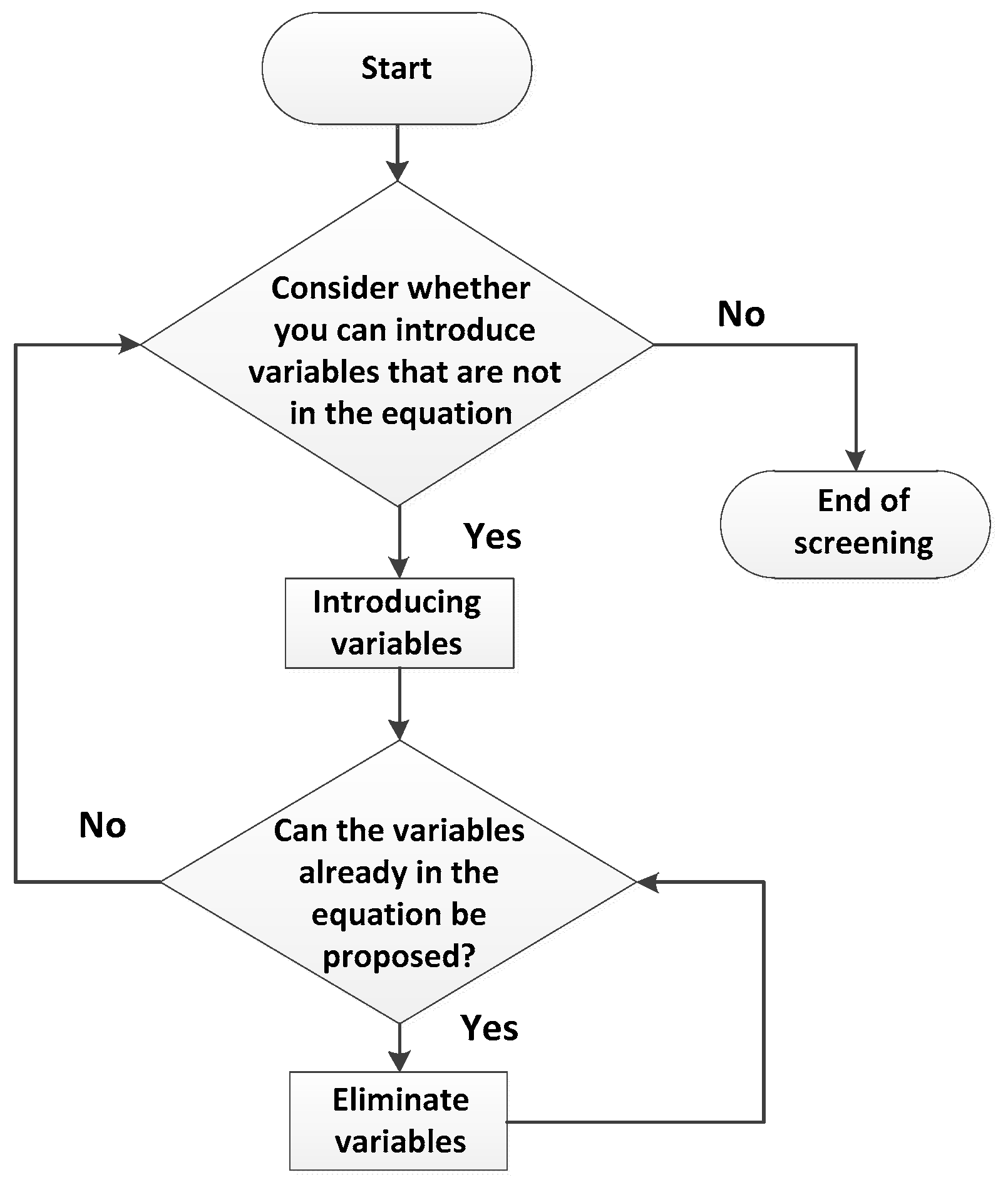
The stepwise regression algorithm is a widely used regression algorithm [24]. Its basic idea is to introduce the independent variables one by one, and the sequence of independent variables influences the dependent variable Y significantly. Each time, the old independent variables are verified one by one while a new independent variable is input. The insignificantly independent variables in the current equation are removed one by one from the independent variables that have the least impact on the dependent variable Y, until you can’t introduce new arguments. Finally, the independent variables retained in the regression equation all have a significant impact on the dependent variable Y, while independent variables that are not in the regression equation have an insignificant effect on Y. Such a regression equation is the optimal equation. The basic steps of stepwise regression can be described in Figure 1.

Assuming that there are m independent variables and n groups of observations, the linear regression model of m elements can be shown as Formula (6):

$$y_i={\beta }_0+{\beta }_1{x}_{i1}+{\beta }_j{x}_{ij}+{\beta }_m{x}_{im}+e_i$$

(6)

where i = 1, 2, …, n represents the i-th observation, j = 1, 2, …, m represents the j-th independent variable, β_j is the partial regression coefficient, and e_i is the random error.

Firstly, the data is normalized, and the average values $\overline{x_j}=\frac{1}{n}{\sum }_{i=1}^n{x}_{ij}, \overline{y}=\frac{1}{n}{\sum }_{i=1}^n{y}_i$, and the standard value σ_xj and σ_y are calculated; then, the correlation coefficient of x_j and y are calculated as $R={\left(r_{ij}\right)}_{M\times M}$. Here, M is the number of all variables including independent variables, and the last row and last column are the correlation coefficients of respective variables and dependent variables. Each independent variable has a significant effect on the dependent variable, and the sum of the squared error of the partial regression is the largest. The inverse transform is used to transform the correlation coefficient matrix, and the previously selected independent variables are tested. If it is not significant, the independent variable will be removed. The process is repeated until all the introduced independent variables have a significant effect on the dependent variable. If k − 1 is reached and m − 1 independent variables are selected at the same time, the following four steps can be taken in step k.

First of all, the partial determination coefficient not selected from the independent variables is calculated according to Formula (7):

$$U_{pi}^{\left(k\right)}=\frac{{\left[r_{im}^{\left(k-1\right)}\right]}^2}{r_{ii}^{\left(k-1\right)}}$$

(7)

where i is an independent variable that has not yet been selected, and $r_{ii}$ represents the i column element of row i on the diagonal line of the correlation coefficient matrix.

Secondly, we compare and find the independent variable x₁ with the largest partial determination coefficient using Formula (8):

$$U_{p1}^{\left(k\right)}=max\left(U_{pi}^{\left(k\right)}\right)$$

(8)

Thirdly, we test the significance of partial regression x₁, as shown in Formula (9):

$$F=\frac{U_{p1}^{\left(k\right)}}{\left(r_{MM}^{\left(k-1\right)}-U_{P1}^{\left(K\right)}\right)/\left(M-m-1\right)}$$

(9)

If the result of the F-test is not significant, then there is no x₁ available for introduction, and the regression is terminated. On the contrary, if the result of the F-test is significant, x₁ is selected, and the r^(k−1) array is inversely transformed into r^(k). The process is shown by Equations (10)–(13).

$$r_{uu}^{\left(k\right)}=\frac{1}{r_{uu}^{\left(k-1\right)}} \left(i=u,j=u\right)$$

(10)

$$r_{uj}^{\left(k\right)}=\frac{r_{uj}^{\left(k-1\right)}}{r_{\mathrm{uu}}^{\left(k-1\right)}} \left(i=u,j\ne u\right)$$

(11)

$$r_{iu}^{\left(k\right)}=\frac{-r_{iu}^{\left(k-1\right)}}{r_{uu}^{\left(k-1\right)}} \left(i\ne u,j=u\right)$$

(12)

$$r_{ij}^{\left(k\right)}=\frac{r_{ij}^{\left(k-1\right)}-r_{iu}^{\left(k-1\right)}{r}_{uj}^{\left(k-1\right)}}{r_{uu}^{\left(k-1\right)}} \left(i\ne u,j\ne u\right)$$

(13)

Last but not least, if x₁ is selected, the partial determination coefficient of the previously selected independent variable x₁ is the same as the value obtained in second step. The F-test is performed on the previously selected independent variable x₁, as shown in Formula (14):

$$F=\frac{U_{pi}^{\left(k\right)}}{r_{MM}^{\left(R\right)}/\left(M-m-1\right)}$$

(14)

where $r_{MM}^{\left(k\right)}$ is the sum of the square error of the standard deviation regression. For the selected x₁, if the dependent variable is significant, we should leave the significant independent variable for the dependent variable, and the process jumps to the first step. If there is an insignificant existence, the independent variable with the smallest deviation coefficient is defined as x₁, the r^(k) matrix is re-transformed, and the program jumps to the first step. The steps mentioned above are repeated until all the significantly independent variables are introduced, and all the non-significantly independent variables are eliminated, so as to obtain the regression equation of the relationship between the independent variable and the dependent variable.

2.3.3. Neural Network Model

A neural network with a hidden layer is used in this study. The full horizontal connection is achieved throughout the network, while the neurons in each layer between the verticals are disconnected. The network is a feed-forward network trained by the error back-propagation algorithm under the minimum error between the actual output and the expected output of the network. The multi-layer connection weights and thresholds of the network are corrected from the back to the front layer. This error back-propagation correction continues, and the correct rate of response of the neural network to the input mode is also rising. The structure of the network is given in Figure 2.

When constructing the neural network model, a random value in the range of (−1,1) to each connection weight and threshold is first assigned; then, the vector $P_k=\left(p_1,p_2,\dots ,p_n\right)$ and the expected output are input as the training samples. The vector $Q_k=\left(q_1,q_2,\dots ,q_i\right)$ is provided to the network. Then, the input vector P_k, the connection weight $v_{ij}$, and the threshold ${\theta }_j$ are used to calculate the input of each unit of the hidden layer. Then, the input is used to calculate the output of each unit of the hidden layer by the transfer function f:

$$O_j=f\left({\displaystyle \sum }_{i=1}^n{v}_{ij}{p}_i-{\theta }_j\right)$$

(15)

where i is the dimension of the input layer i = (1, 2, ..., n). Then, the output $O_j$ is used to connect weights ${\omega }_{jt}$ with ${\psi }_t$ thresholds of the hidden layer to calculate the output of each unit of the hidden layer. Then, we use the output of the hidden layer to calculate the output of the output layer through the transfer function f; the actual output of the network is given in Formula (16):

$$Y_t=f\left({\displaystyle \sum }_{j=1}^p{\omega }_{jt}{O}_j-{\psi }_t\right)$$

(16)

where j is the j-th dimension of the hidden layer. In Equations (15) and (16), the transfer function f is usually expressed by a sigmoid-type function:

$$f\left(x\right)=\frac{1}{1+e^{-x}}$$

(17)

The expected output vector $O_i$ and the actual output vector Y_t are used to calculate the error of the output layer.

$$d_t^k=\left(q_t^k-Y_t\right)f^{’}\left({\displaystyle \sum }_{j=1}^p{\omega }_{jt}{O}_j-{\psi }_t\right)$$

(18)

where f’ is the derivative of the output layer function. Then, the connection weight ${\omega }_{jt}$ and the output of each unit of the hidden layer are used to calculate the correction error of the hidden layer.

$$e_j^k=\left({\displaystyle \sum }_{t=1}^q{\omega }_{jt}{d}_t\right)f’\left({\displaystyle \sum }_{i=1}^n{v}_{ij}{p}_i-{\theta }_j\right)$$

(19)

After obtaining the above correction error, the error is used to correct the connection weight and threshold between the output layer and the hidden layer and between the hidden layer and the input layer. The correction amounts are:

$$\Delta {\omega }_{jt}=\alpha d_t^k{O}_j$$

(20)

$$\Delta {\psi }_t=\alpha d_t^k$$

(21)

where 0 < α < 1.

$$\Delta v_{ij}=\beta e_j^k{p}_i^k$$

(22)

$$\Delta {\theta }_j=\beta e_j^k$$

(23)

where 0 < β < 1.

We used the TensorFlow tool to implement the models in this paper; a three-layer multi-input and single-output neural network with one hidden layer is adopted to establish a prediction model. However, if the number of neurons in the hidden layer is very large, the calculating amount will increase, and the over-fitting problem will easily occur. If the number of neurons is too small, the network performance will be affected, and the expected effect will not be achieved. Therefore, it is necessary to have a reasonable number of neurons. Through many experiments, we finally selected 20 neurons in the hidden layer, and employed the momentum method to define the optimizer and get the prediction results.

Meanwhile, we constructed a deep neural network (DNN) model because it often provides better performance than general neural networks with one hidden layer. The DNN model adopted in this paper is implemented by TensorFlow, and is composed of five hidden layers and one output layer.

3. Results and Discussion

3.1. Preprocessing and Feature Selection

In this paper, features are selected by their contribution, which is calculated by seven feature selection methods on the H dataset and G dataset mentioned above, which are chosen in descending order and in accordance with the rule that the sum of contribution values of selected features is over 95% (see

Table 1. Contribution of features by different selection methods for the G dataset.

Features	Linear Regression	Ridge Regression	Lasso Regression	Random Forest	Correlation	Stability	AVG
a1	0.0240	0.0071	0.0248	0.0022	0.0529	0.2518	0.0605
a2	0.0102	0.0608	0.0943	0.0019	0.0489	0.1027	0.0531
a3	0.0061	0.1091	0.0000	0.0007	0.0746	0.0489	0.0399
a4	0.0928	0.0402	0.1069	0.0150	0.0697	0.0440	0.0614
a5	0.0002	0.0520	0.0000	0.0168	0.0554	0.0073	0.0219
a6	0.3179	0.0031	0.0000	0.0000	0.0688	0.0122	0.0670
a7	0.0121	0.0402	0.0000	0.1065	0.0697	0.0245	0.0422
a8	0.0023	0.0351	0.2630	0.0080	0.0256	0.0685	0.0671
a9	0.0084	0.1084	0.2995	0.5773	0.0314	0.0000	0.1708
a10	0.0097	0.1017	0.0000	0.0916	0.0313	0.0000	0.0391
a11	0.0003	0.1120	0.2115	0.0828	0.1571	0.2689	0.1388
a12	0.0371	0.1986	0.0000	0.0025	0.0567	0.0049	0.0500
a13	0.0514	0.0398	0.0000	0.0004	0.1019	0.1222	0.0526
a14	0.0012	0.0046	0.0000	0.0827	0.0199	0.0024	0.0185
a15	0.0015	0.0007	0.0000	0.0000	0.0026	0.0000	0.0008
a16	0.0952	0.0400	0.0000	0.0116	0.0697	0.0220	0.0398
a17	0.3296	0.0467	0.0000	0.0000	0.0639	0.0196	0.0766

and

Table 2. Contribution of features by different selection methods for the H dataset.

Features	Linear Regression	Ridge Regression	Lasso Regression	Random Forest	Correlation	Stability	AVG
a1	0.0165	0.0147	0.0000	0.0000	0.0244	0.0748	0.0217
a2	0.0057	0.0173	0.0159	0.0000	0.0230	0.0262	0.0147
a3	0.1262	0.1930	0.2302	0.0000	0.1218	0.2037	0.1458
a4	0.0241	0.0067	0.0550	0.0000	0.0486	0.0037	0.0230
a5	0.0025	0.0345	0.0000	0.0000	0.0680	0.0093	0.0191
a6	0.2952	0.1279	0.0617	0.0000	0.0831	0.0131	0.0968
a7	0.0763	0.0066	0.0027	0.0000	0.0486	0.0019	0.0227
a8	0.0074	0.0153	0.0463	0.0000	0.0151	0.1364	0.0368
a9	0.0501	0.1755	0.2563	0.9221	0.0873	0.2056	0.2828
a10	0.0041	0.0001	0.0959	0.0000	0.0593	0.0206	0.0300
a11	0.0414	0.0952	0.0227	0.0000	0.0996	0.2037	0.0771
a12	0.0565	0.1154	0.1982	0.0012	0.0519	0.0000	0.0705
a13	0.0092	0.0624	0.0000	0.0000	0.0983	0.0486	0.0364
a14	0.0008	0.0005	0.0000	0.0765	0.0390	0.0486	0.0276
a15	0.0003	0.0093	0.0053	0.0000	0.0024	0.0000	0.0029
a16	0.1010	0.0066	0.0000	0.0000	0.0486	0.0000	0.0261
a17	0.1826	0.1192	0.0099	0.0000	0.0809	0.0037	0.0660

). The other features whose total sum of contribution values is less than 5% are considered to have a lesser influence on the results, and can be ignored.

Here, a1–a17 represent 17 features of Level, Speed, GTST, GTS, CPPTS, STP, SRP, GGS, FF, ABBTCS, GTCOAP, EP, HPTEP, TCSTCS, TCS, PRS, and PTP, respectively. The data marked in bold in the tables is the final selected variable attribute corresponding to it.

The process of feature selection and data processing for the HPTET temperature are same to that of the GTCOAT temperature, which is given in Table 2.

3.2. Results of GTCOAT Temperature Prediction.

In the present section, we predicted the test dataset according to the correlation coefficient obtained from the training data experiment, and compared the predicted results with the actual data. Three error analysis methods were employed, which are the actual error, absolute error, and relative error. Then, we drew two kinds of error graph, namely the actual error and relative error. Meanwhile, we compared their mean absolute error (MAE) and mean average relative error (MARE), and comprehensively analyzed the prediction effect. By comparing the seven feature selection methods for the time series, we found that for the GTCOAT temperature, the AVG feature selection method had the best prediction results (see

Table 3. Results of models for forecasting the GTCOAT temperature. ARDL: autoregressive distributed lag time series model, DNN: deep neural network, LR1: time-series model with 1 lag, MAE: mean absolute error, MARE: mean average relative error, NN: neural network, SR: stepwise regression.

Feature	Error Measures	ARDL				LR	NN	DNNc	SR
		LR1	LR5	LR10	LR15
AVG	MAE MARE	2.3686 0.0037	1.3055 0.0020	1.0542 0.0016	1.0491 0.0016	2.4770 0.0039	9.3936 0.0141	17.9556 0.0271	2.7024 0.0042
Corr	MAE MARE	3.3785 0.0050	3.1014 0.0046	2.7143 0.0040	2.7087 0.0039	3.4136 0.0051	52.1559 0.0683	17.9556 0.0271
Lasso	MAE MARE	3.4321 0.0050	2.9558 0.0043	2.5779 0.0037	2.5703 0.0037	3.4511 0.0050	53.3080 0.0699	15.5496 0.0233
Lr	MAE MARE	3.6609 0.0053	3.3412 0.0049	2.7627 0.0040	2.7579 0.0040	3.7152 0.0054	46.1879 0.0575	20.2862 0.0306
RF	MAE MARE	20.9895 0.0312	12.5970 0.0183	6.0679 0.0088	6.0698 0.0088	21.8452 0.0328	41.7166 0.0572	28.8141 0.0460
Ridge	MAE MARE	3.3291 0.0049	2.9402 0.0043	2.5979 0.0038	2.5888 0.0038	3.3844 0.0049	21.3081 0.0335	27.7896 0.0405
Stability	MAE MARE	7.7299 0.0111	5.4886 0.0077	4.9152 0.0069	4.9091 0.0068	8.5276 0.0122	47.2233 0.0600	17.8013 0.0268

). Moreover, the ARLD model with 15 lag steps has the smallest prediction error among all the models, whose MAE value is 1.0491 and MARE value is 0.0016. Table 3 shows that the DNN model is more accurate than the NN model, so the prediction accuracy can be improved by increasing the number of hidden layers. However, at the same time, it brings many problems, such as over-fitting and so on.

The data in Table 3 marked in black bold color is the data obtained under the best selected features of the final selection. The abbreviations for the following prediction methods make the table simpler and clearer.

• LR1: Time-Series Model with 1 lag.
• NN: Neural Network Model.
• DNN: Deep Neural Network Model.
• SR: Stepwise Regression Model.

Due to the large amount of data in this experiment, we have to select continuous data to visualize the results. Figure 3 and Figure 4 respectively show the actual error and relative error between the predicted and actual values of all models. Figure 3 shows that the actual error range of the ARDL model with 15 lag steps is the smallest, most of which are concentrated between –3 and 3. At the same time, Figure 4 shows that the relative error of this model is the smallest, mostly less than 0.06. Therefore, we can conclude that the ARDL model with 15 lag steps has the best results for predicting the GTCOAT temperature.

3.3. Results of HPTET Temperature Prediction.

Similarly, the process of models for predicting the HPTET temperature equals to that for predicting the GTCOAT temperature. The results of all models for predicting the HPTET temperature are shown in

Table 4. Results of models for forecasting the HPTET temperature.

Feature	Error Measures	ARDL				LR	NN	DNN	SR
		LR1	LR5	LR10	LR15
AVG	MAE MARE	3.3385 0.0049	2.8086 0.0041	2.5311 0.0037	2.5255 0.0037	3.3548 0.0049	66.4863 0.0855	50.5350 0.0645	20.8675 0.0317
Corr	MAE MARE	3.3785 0.0050	3.1014 0.0046	2.7143 0.0040	2.7087 0.0039	3.4136 0.0051	52.1559 0.0683	33.5700 0.0502
Lasso	MAE MARE	3.4321 0.0050	2.9560 0.0043	2.5779 0.0037	2.5703 0.0037	3.4511 0.0050	53.3080 0.0699	54.1260 0.0700
Lr	MAE MARE	3.6609 0.0053	3.3412 0.0049	2.7627 0.0040	2.7579 0.0040	3.7152 0.0054	46.1879 0.0575	38.9521 0.0615
RF	MAE MARE	20.9895 0.0312	12.5970 0.0183	6.0679 0.0089	6.0699 0.0088	21.8452 0.0328	41.7166 0.0572	326.0747 0.4034
Ridge	MAE MARE	3.3290 0.0049	2.9402 0.0043	2.5979 0.0038	2.5888 0.0038	3.3844 0.0049	21.3081 0.0335	42.6881 0.0575
Stability	MAE MARE	7.7299 0.0111	5.4886 0.0077	4.9152 0.0069	4.9091 0.0069	8.5276 0.0122	47.2233 0.0600	48.1805 0.0612

, which shows that the MAE and the MARE of the ARDL model with 15 lag steps is the smallest after the AVG feature selection method. The MAE and MARE of this model are 2.5255 and 0.0037, respectively.

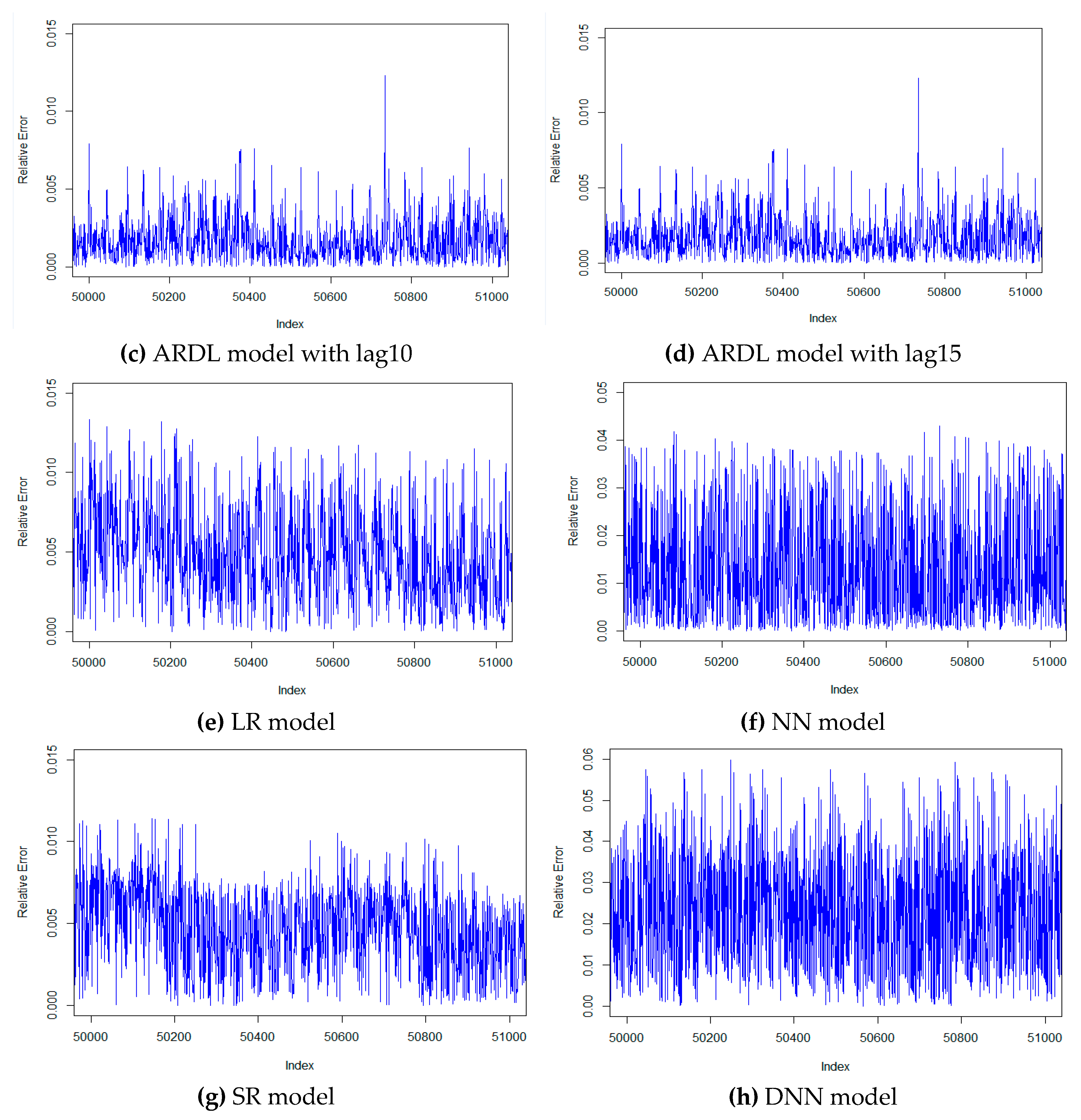
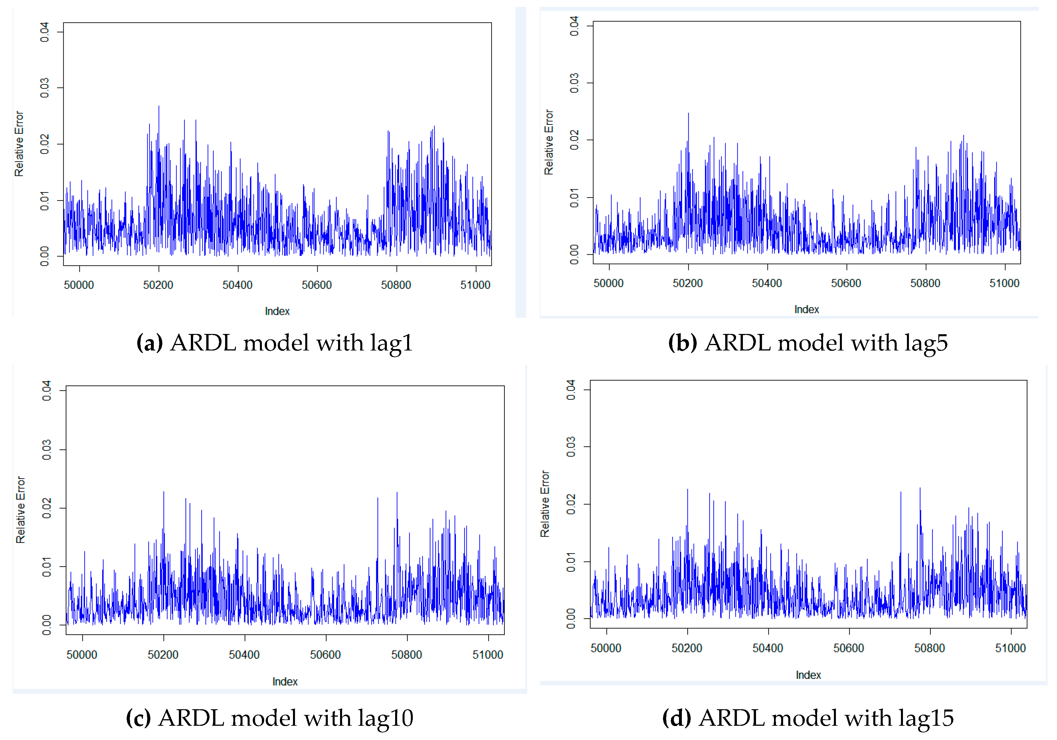
Subsequently, we also select 1000 continuous records to visualize the results. Figure 5 and Figure 6 showed the actual error and relative error of all the models for predicting the HPTET temperature. Figure 5 shows that the actual error range of the ARDL model with 15 lag steps is the smallest, most of which are concentrated between –10 and 10. At the same time, from Figure 6, we can easily find that the relative error of this model is the smallest, mostly less than 0.02. Therefore, we can conclude that the ARDL model with 15 lag steps has the best prediction results for predicting the HPTET temperature.

3.4. Discussions

Based on the above experimental results, we know that the ARDL model with the AVG feature selection method shows better results for forecasting both the GTCOAT and HPTET temperatures. For the GTCOA temperature, when the ARDL model has one lag step, the AVG feature selection method shows that the MAE is 2.3686 and an MARE of 0.0037. With 5 lag steps, the MAE is 1.3055 and the MARE is 0.0020. With 10 lags, the MAE is 1.0542 and the MARE is 0.0016. With 15 lags, the MAE is 1.0491 and the MARE is 0.0016. Among the rest of the models, the MAE and MARE of the multiple linear regression method are 2.4770 and 0.0039, respectively. The MAE and MARE of the stepwise regression model are 2.7024 and 0.0042, respectively. The MAE and MARE of the NN model are 9.3936 and 0.0141, respectively. The MAE and MARE of the DNN model with the Lasso feature selection method are 33.5700 and 0.0502, respectively.

For the HPTET temperature, when the ARDL model has one lag step, the MAE and the MARE are 3.3385 and 0.0049, respectively. With 5 lag steps, the MAE and the MARE are 2.8086 and 0.0041, respectively. With 10 lags, the MAE and MARE are 2.5311 and 0.0037, respectively. With 15 lags, the MAE and MARE are 2.5255 and 0.0037, respectively. Among the rest of the models, the MAE and MARE of the linear regression model are 3.3548 and 0.0049, respectively. The MAE and MARE of the stepwise regression model are 20.8675 and 0.0317, respectively. The MAE and MARE of the NN model are 66.4863 and 0.08556, respectively. The MAE and MARE of the DNN model with the Corr feature selection method are 15.5496 and 0.0233, respectively.

According to the analysis mentioned above, we know that the ARGL model with 15 lags under AVG feature selection has the smallest error and the best prediction accuracy. The reason is that the remote sensing data from ships is time series, which means that the time-series correlation prediction model is more effective. In addition, we analyzed the running time of these models. Our experiments are carried out on a 64-bit Windows 7 operation system computer, in which the CPU is an Intel(R) Core(TM) i7-3370 cpu @ 3.40GHz 3.40GHz. All the models are sorted by the running time in ascending order: The LR model takes about 55 seconds, the ARDL models with 1 lag step, 5 lag steps, 10 lag steps, and 15 lag steps respectively take about 60 seconds, 75 seconds, 95 seconds, and 110 seconds; the NN model takes about 460 seconds; lastly, the DNN model takes about 1500 seconds, which shows that the performance of the neural network model is worse than the ARDL model, and the more complex the network is, the more time it takes.

Some potential failures of the propulsion system can be found by the difference between the actual temperature and the predicted temperature, since sudden temperature changes are mainly caused by device failure. In actual voyage, it not only helps the crew to identify the location of the faults, but also automatically reminds them to focus on warnings of possible failures. The maintenance personnel only need to locate the specific parts of the abnormal situation in time and carry out inspection and maintenance, which can greatly reduce the workload of the crew and reduce the operation and maintenance cost of the ship.

4. Conclusions

Timely potential fault prognostics and early warnings in advance can effectively reduce the cost of operation and maintenance of ships, thereby further saving energy and reducing the cost of the operation and maintenance of ships. Device failure is often accompanied by sudden changes in temperature. Therefore, we focused on the temperature forecast of ship propulsion devices in this paper, and based on the states and position information of the ship transmitted to the shore at regular intervals, carried out a series of analysis and mining on the collected data, and constructed the several forecasting models. It is essential to compare these models because we lack prior knowledge, and the results can be summarized as follows:

(1) Compared with other feature selection methods, the AVG feature selection method shows the best effect.

(2) When forecasting the GTCOAT temperature, the MAE values of the ARDL model with 15 lag steps, the linear regression model, the stepwise regression model, the NN model, and the DNN model are 1.0491, 2.4770, 2.7024, 9.3936, and 15.5496, respectively while the MARE values of these models are 0.0016, 0.0039, 0.0042, 0.0141, and 0.0233 respectively. Similarly, when forecasting the HPTET temperature, the MAE values of the ARDL model with 15 lags, the linear regression model, the stepwise regression model, the NN model, and the DNN model are 2.5255, 2.4770, 20.8675, 66.4863, and 33.5700, respectively, while the MARE values of these models are 0.0037, 0.0039, 0.0317, 0.0855, and 0.0502, respectively.

The results show that the temperature forecast of the ship propulsion devices displays the linear features in two aspects: One is that the ARDL model has the most stable results and the highest accuracy. Another is that the NN model often shows better results for solving non-linear problems, but in this case, it shows worse results than the two other models.

(3) The forecasted temperatures can remind crew on board to discover potential failures timely, which will contribute to correct maintenance decisions and suggestions, so as to take effective measures to quickly troubleshoot the faults. Consequently, it is conducive to energy conservation, emission reduction, environmental protection, and sustainable energy development.

In this paper, we only predict the temperature of the ship propulsion system, but do not analyze the acceptable margin of error and how to identify the fault of ship propulsion devices because of the lack of empirical knowledge. In the future, we will try our best to improve the precision, reduce the training time, and discuss the reasonable margin of error.

References

- Ji, Y.L.; Sun, Y.Q.; Zhang, H.P.; Zhang, Y.D.; Chen, H.Q. Novel Ship Propulsion System. Chin. J. Mech. Engin. 2009, 22, 198–206. [Google Scholar] [CrossRef]
- Onwuegbuchunam, D.E.; Ebe, T.E.; Okoroji, L.I. An Analysis of Ship-Source Marine Pollution in Nigeria Seaports. J. Mar. Sci. Eng. 2017, 5, 39. [Google Scholar] [CrossRef]
- Iodice, P.; Langella, G.; Amoresano, A. A numerical approach to assess air pollution by ship engines in manoeuvring mode and fuel switch conditions. Energy Environ. 2017, 28, 827–845. [Google Scholar] [CrossRef]
- Kim, M.; Park, D.W. A study on the green ship design for ultra large container ship. J. Mar. Sci. Eng. 2015, 21, 558–570. [Google Scholar] [CrossRef]
- Gudehus, T.; Kotzab, H. Economic Ship Travel Speed and Consequences for Operating Strategies of Container Shipping Companies. In Proceedings of the 4th International Conference on Dynamics in Logistics (LDIC), Bremen, Germany, 10–14 February 2014; pp. 407–415. [Google Scholar]
- Feng, D.H.; Li, Y.H. Research on Intelligent Diagnosis Method for Large-Scale Ship Engine Fault in Non-Deterministic Environment. Pol. Marit. Res. 2017, 24, 200–206. [Google Scholar] [CrossRef] [Green Version]
- Tang, G.G.; Fu, X.D.; Chen, N. Ship Power Plant Remote Fault Diagnosis System Based on B/S and C/S Architecture. Ship Eng. 2018, 40, 66–71. [Google Scholar]
- Yang, Y.F.; Feng, J. Fault Pattern Recognition and State Prediction Research of Ship Power Equipment Based on HMM-SVR. Ship Eng. 2018, 40, 68–72, 97. [Google Scholar]
- Wu, J.P.; Peng, H.; Ohtsu, K. Ship’s tracking control based on nonlinear time series model. Appl. Ocean Res. 2012, 36, 1–11. [Google Scholar] [CrossRef]
- McCullough, M.; Sakellariou, K.; Stemler, T.; Stemler, T. Regenerating time series from ordinal networks. Chaos. 2017, 27. [Google Scholar] [CrossRef]
- Cinar, Y.G.; Mirisaee, H.; Goswami, P. Period-aware content attention RNNs for time series forecasting with missing values. Neurocomput. 2018, 312, 177–186. [Google Scholar] [CrossRef]
- Yang, S.; Liu, J. Time-Series Forecasting Based on High-Order Fuzzy Cognitive Maps and Wavelet Transform. IEEE Trans. Fuzzy Syst. 2018, 26, 3391–3402. [Google Scholar] [CrossRef]
- Coraddu, A.; Oneto, L.; Ghio, A. Machine learning approaches for improving condition- based maintenance of naval propulsion plants. Proc. Inst. Mech. Eng. Part M J. Eng. Marit. Environ 2016, 230, 136–153. [Google Scholar] [CrossRef]
- Cipollini, F.; Oneto, L.; Coraddu, A.; Murphy, A.J.; Anguita, D. Condition-based maintenance of naval propulsion systems with supervised data analysis. Ocean Eng. 2018, 149, 268–278. [Google Scholar] [CrossRef]
- Yerel, S.; Ersen, T. Prediction of the Calorific Value of Coal Deposit Using Linear Regression Analysis. Energy Sour. Part A Recov. Util. Environ. Eff. 2013, 35, 976–980. [Google Scholar] [CrossRef]
- Liu, X.Q.; Gao, F.; Xu, J.W. Linearized Restricted Ridge Regression Estimator in Linear Regression. Commun. Stat.-Theory Methods 2012, 41, 4503–4514. [Google Scholar] [CrossRef]
- Chang, L.; Roberts, S.; Welsh, A. Robust Lasso Regression Using Tukey’s Biweight Criterion. Technometrics 2018, 60, 36–47. [Google Scholar] [CrossRef]
- Scornet, E. Random Forests and Kernel Methods. IEEE Trans. Inf. Theory 2016, 62, 1485–1500. [Google Scholar] [CrossRef] [Green Version]
- Díaz-Uriarte, R.; DeAndres, S.A. Gene selection and classification of microarray data using random forest. BMC Bioinform. 2006, 7, 1–13. [Google Scholar] [CrossRef]
- Zhang, Y.; Liu, T.; Li, K.F.; Zhang, J.W. Improved visual correlation analysis for multidimensional data. J. Vis. Lang. Computing 2017, 41, 121–132. [Google Scholar]
- Wen, M.L.; Qin, Z.F.; Kang, R. Sensitivity and stability analysis in fuzzy data envelopment analysis. Fuzzy Optim. Decis. Mak. 2011, 10, 1. [Google Scholar] [CrossRef]
- Acikkar, M.; Sivrikaya, O. Prediction of gross calorific value of coal based on proximate analysis using multiple linear regression and artificial neural networks. Turk. J. Electr. Eng. Comput. Sci. 2018, 26, 2541–2552. [Google Scholar] [CrossRef]
- Yue, S.P. Modeling of Engine Parameters for Condition-Based Maintenance of the MTU Series 2000 Diesel Engine. Master’s Thesis, Naval Postgraduate School, Monterey, CA, USA, September 2016. [Google Scholar]
- Agostinelli, C. Robust stepwise regression. J. Appl. Stat. 2002, 29, 825–840. [Google Scholar] [CrossRef] [Green Version]
Figure 1.
Steps of the stepwise regression algorithm.
Figure 2.
The structure of the neural network.
Figure 3.
Actual error of all models for predicting the GTCOAT temperature. Figure 3 contains eight graphs, which were listed as follows: (a) ARDL model with lag 1, (b) ARDL model with lag 5, (c) ARDL model with lag 10, (d) ARDL model with lag 15, (e) LR model, (f) NN model, (g) SR model, (h) DNN model.
Figure 4.
Relative error of all models for predicting the GTCOAT temperature. Figure 4 contains eight graphs, which were listed as follows: (a) ARDL model with lag 1, (b) ARDL model with lag 5, (c) ARDL model with lag 10, (d) ARDL model with lag 15, (e) LR model, (f) NN model, (g) SR model, (h) DNN model.
Figure 5.
Actual error of ARDL model for predicting the HPTET temperature. Figure 5 contains eight graphs, which were listed as follows: (a) ARDL model with lag 1, (b) ARDL model with lag 5, (c) ARDL model with lag 10, (d) ARDL model with lag 15, (e) LR model, (f) NN model, (g) SR model, (h) DNN model.
Figure 6.
Relative error of ARDL model for predicting the HPTET temperature with different lag steps. Figure 6 contains eight graphs, which were listed as follows: (a) ARDL model with lag 1, (b) ARDL model with lag 5, (c) ARDL model with lag 10, (d) ARDL model with lag 15, (e) LR model, (f) NN model, (g) SR model, (h) DNN model.