Hierarchical Clustering Approach for Selecting Representative Skylines


1
Department of Mathematics and Computer Science, Eindhoven University of Technology, 5612 AZ Eindhoven, The Netherlands
2
Department of Computer Science, Chungbuk National University, Cheongju 28644, Korea
*
Author to whom correspondence should be addressed.
Information 2019, 10(3), 96; https://0-doi-org.brum.beds.ac.uk/10.3390/info10030096
Submission received: 3 January 2019
/
Revised: 23 February 2019
/
Accepted: 26 February 2019
/
Published: 5 March 2019
Abstract
:Recently, the skyline query has attracted interest in a wide range of applications from recommendation systems to computer networks. The skyline query is useful to obtain the dominant data points from the given dataset. In the low-dimensional dataset, the skyline query may return a small number of skyline points. However, as the dimensionality of the dataset increases, the number of skyline points also increases. In other words, depending on the data distribution and dimensionality, most of the data points may become skyline points. With the emergence of big data applications, where the data distribution and dimensionality are a significant problem, obtaining representative skyline points among resulting skyline points is necessary. There have been several methods that focused on extracting representative skyline points with various success. However, existing methods have a problem of re-computation when the global threshold changes. Moreover, in certain cases, the resulting representative skyline points may not satisfy a user with multiple preferences. Thus, in this paper, we propose a new representative skyline query processing method, called representative skyline cluster (RSC), which solves the problems of the existing methods. Our method utilizes the hierarchical agglomerative clustering method to find the exact representative skyline points, which enable us to reduce the re-computation time significantly. We show the superiority of our proposed method over the existing state-of-the-art methods with various types of experiments.
1. Introduction
In data mining and data analysis, a multi-criteria analysis is a conventional method to address the problems of real-life applications from recommendation systems to decision making. One of the commonly used multi-criteria analysis methods is the skyline query. The skyline query enables obtaining of interesting and dominant data points from the given dataset [1]. For example, consider a hotel recommendation system. Assume that a system has information regarding the various hotels in a particular location with attributes, including price and distance (i.e., distance from the beach). In most cases, the user would prefer hotels with a low price and those closest to the beach. Here, the skyline query returns the hotels that satisfy user preferences. Due to its usefulness, the skyline query is extensively studied in many fields [2].
Formally, the skyline query can be defined as follows. Data point pi of a d-dimensional set of data points P with the attribute value of pi.vj dominates data point pk (1 ≤ (i, k) ≤ |P|, 1 ≤ j ≤ d, i ≠ k), if every attribute value of pi is equal or less than pk’s (pi.vj ≤ pk.vj), and if there exists an attribute value, which is less than pk’s (pi.vj < pk.vj), then pi dominates the pk (pi < pk).
Figure 1 illustrates an example of finding skyline points in two-dimensional space. Here, Figure 1a visualizes the input data set in two-dimensional space, which contains 16 data points. Figure 1b shows skyline points obtained from Figure 1a. Assume that Figure 1 depicts the hotels mentioned earlier. In this case, A1 indicates the distance from the beach and A0 indicates hotel prices. From Figure 1b, it is easy to see that the highlighted points represent hotels with a low price and a distance closest to the beach.
Generally, in the low-dimensional dataset, the skyline query returns a small number of skyline points. However, as the dimensionality of the dataset increases, the number of skyline points also increases. Depending on data distribution and dimensionality, most of the data points may become skyline points. Koizumi et al. [3] introduced a skyline query processing technique, called BJR-Tree. In the research, the authors conducted extensive experiments that show the skyline points’ ratio in various dimensionality and three different data distribution, namely uniform, correlated, and anti-correlated. Specifically, the experiment results for uniform and correlated datasets demonstrate that more data points become skyline points from fifteen to the twenty-five-dimensional dataset. The situation worsens for the anti-correlated dataset, where more data points become skyline points starting from eight dimensions. This study demonstrates the lack of skyline query processing methods when the dataset is high-dimensional. With the emergence of big data applications, where the data distribution and dimensionality is a significant problem, obtaining representative skyline points among resulting skyline points is necessary.
There have been several methods that focused on extracting representative skyline points with various success [4,5,6]. These methods utilize a specific global threshold value. However, without prior knowledge of the given dataset, the user must guess or iteratively increase the global threshold value, which leads to a problem of re-computation. In other words, once the global threshold value for representative skyline points changes, most of the existing methods reset the whole process and begin over again. As a result, it increases the overall processing time required for finding representative skyline points.
This problem can become significant in real-world applications as well. For example, assume that a hotel recommendation system that recommends the k representative hotels depending on the user given value. Suppose that the system stores hotels with low prices and distance closest to the beach, as shown in Figure 1b. Let us assume that user1, user2, and user3 connected to the system concurrently requested k = 3, k = 1, and k = 5 hotels, respectively. The system recommends three representative hotels (k = 3) first and returns the result to the user1. Further, the system must begin a new process and re-compute a single representative hotel for user2. Finally, the system re-computes once again to show the five representative hotels to the user3. The overall computational time of these methods increases as the number of requests increases. Moreover, certain existing representative skyline query processing methods [4,5] find an approximate result when d ≥ 3.
In this paper, we propose a new representative skyline query processing method, which solves the problems of existing methods. More specifically, our contributions are as follows:
- We propose a method for selecting the representative skyline points that uses the hierarchical agglomerative clustering structure. Here, we define a new distance measurement called θ distance that enables us to obtain a set of top and diverse representative skyline points by configuring the hierarchical agglomerative clustering structure.
- We also show the correctness and efficiency of our proposed method through a comprehensive experimental study.
The rest of the paper is organized as follows. In Section 2, we first review the skyline query processing methods and then discuss the previous work on representative skyline query processing. Further, in Section 3, we describe the proposed method for selecting the representative skyline query processing, which utilizes the hierarchical agglomerative clustering. In Section 4, we demonstrate the result of experiments on both synthetic and real datasets. Finally, in Section 5, we conclude the paper and discuss future work.
2. Related Work
In this section, we first review the skyline query processing methods in Section 2.1 and the representative skyline query processing methods in Section 2.2.
2.1. Skyline Query Processing Methods
There have been numerous methods proposed to process the skyline query efficiently. After Borzsony and Kossmann [7] proposed a naive method of skyline query processing, called Block-Nested-Loops (BNL), several other efficient skyline query processing methods were introduced. We can summarize these methods into three categories: sort, partition, and index-based methods.
Chomicki et al. [8] proposed a method, called Sort-Filter-Skyline (SFS). It uses the same algorithmic pattern as the BNL with an extra preprocessing step. In this preprocessing step, data points P are scored by the monotone scoring function and sorted in ascending order. Unlike the BNL, the SFS algorithm finds the skyline points with less CPU and I/O cost. Godfrey et al. [9] proposed an alternative sort-based skyline query processing method, called Linear-Elimination-Sort-for-Skyline (LESS). This method improves the SFS by introducing an elimination filter. This elimination filter is used during the sorting process to reduce the number of pairwise comparisons of the SFS. On the other hand, Bartolini et al. [10] proposed another extension of the SFS method, which uses stop pointers and reduces the search space.
Partition-based skyline query processing methods divide the whole data space into smaller chunks. Thus, the data can fit into the main memory. Borzsony and Kossmann [7] proposed two different partition-based skyline query processing methods, called D&C and M-Way. The D&C method uses a conventional median split to partition the d-dimensional dataset into 2d partitions. On the other hand, M-Way uses a quantile split to divide the dataset into more specific partitions. Here, both methods first find the local skyline points in each partition, and then, merge the skyline points. This method can reduce the computational time and can be useful in the distributed environments. However, Vlachou et al. [11] argued that such partitioning methods produce empty spaces. To solve the problem, the authors proposed the angle-based skyline query processing method to remove the empty spaces from the search space. Here, to partition the data points according to the certain angular threshold, the algorithm turns the Cartesian coordinates of the data points into hyper-spherical coordinates.
Unlike previous skyline query processing methods, index-based skyline query processing methods utilize the indexing structure to find the skyline points efficiently. Tan et al. [12] proposed to use the Bitmap index to find skyline points. The efficiency of the bitmap relies on the speed of bit-wise operations. However, due to the number of distinct values, a large amount of space is required to create a Bitmap index. Thus, Papadias et al. [13] proposed to use the R-Tree indexing structure to process the skyline query efficiently, called Branch-and-Bound-Skyline (BBS). The R-Tree index creates minimum bounding rectangles (MBR) that contain m to M points. Thus, if any other point dominates the lower left edge of the MBR, then BBS discards the whole MBR. Unlike conventional methods based on the pair-wise comparison, this method enables us to perform a region-wise comparison and find the skyline points efficiently. A different skyline query processing method, which is called Z-Sky, was proposed in [14]. Here, the authors argued that even with the region-wise comparison, BBS still suffers from empty space and overlapping MBR problems. To solve these problems, Z-Sky uses a space-filling Z-curve with B+-Tree that reduces the computational time.
2.2. Representative Skyline Query Processing Methods
There have been numerous representative skyline query processing methods that focused on obtaining the representative skyline point set. We can categorize them into two major groups, namely dominance and distance-based methods. In Section 2.2.1, we review the dominance-based representative skyline query processing methods, and in Section 2.2.2, we discuss the distance-based methods. Finally, in Section 2.2.3, we provide an in-depth analysis of current representative skyline query processing methods.
2.2.1. Dominance-Based Methods
Tao et al. [5] proposed a method, called Maximum-dominance (Max-Dom), to find the top-k dominant representative skyline points from the skyline set S. For that, the authors first find the skyline points S from the data points P. Further, they count the number of dominated data points of each skyline point and store them in corresponding lists in descending order. Finally, k skyline points (p′1 … p′k) from the list is selected as the top-k representative skyline points. On the other hand, Huang et al. [15] proposed a method, to find the representative skyline points, that utilizes the subspace skyline points and called it as δ-Skyline (δ-Sky). Here, if the user given threshold δ is less than the cardinality of skyline points (δ < |S|), then δ-Sky calculates the subspace skyline points recursively until the number of skyline points is less or equal to δ (δ ≥ |S|). In the performance evaluation of the proposed method, the authors demonstrated that the δ-Sky method is more efficient if the input is a pre-built skycube [16], instead of skyline points S.
Xia et al. [17] proposed a ε-Sky method. In this method, instead of making the comparison on the skyline points or the data points, the authors perform the skyline region partitioning based on the ε value. The range of ε value is [−1.0, 1.0]. There is a special case when the ε = 0 (i.e., all the skyline points become representative skyline points). Thus, depending on the ε value, the ε-Sky moves the skyline region towards the origin of the data space or maximum value. Suppose that the data point values are in the unit range [0.0, 1.0]d, then ε < 0, it moves the skyline region towards the [0.0, 0.0]d. On the other hand, when ε > 0, it moves the skyline region towards the [1.0, 1.0]d, and returns the data points on the left side of the skyline region as the representative skyline points. Koltun et al. [18] used the same notation ε to find the representative skyline points, called approximately dominating representatives (ADR). The proposed method is similar to the density-based clustering method (i.e., DBSCAN), which creates a number of circles with the radius of ε on the skyline points. In this method, the center of the circles become the representative skyline points.
2.2.2. Distance-Based Methods
Most of the distance-based methods create the groups of similar skyline points and sample the representative skyline points from each group. Nanongkai et al. [19] proposed the method of finding representative skyline points using a distance-based measurement (e.g., Greedy). In their research, the authors have discovered that dominance-based methods, such as Max-Dom, cannot guarantee to show the full contour of the skyline points. Thus, the authors proposed a number of algorithms that choose the k representative skyline points. These k representative skyline points are the skyline points that minimize the maximum distance between the skyline points. However, their method only finds exact representatives in d = 2. When d ≥ 3, the algorithm becomes NP-hard, and thus, only finds the approximate representative skyline points.
Zhao et al. [6] proposed an alternative distance-based method, which utilizes the k-medoids clustering algorithm to find the representative skyline points, called Call-to-Order. Based on the user preferences, the method samples the skyline points using the TA algorithm and creates k clusters. However, it still suffers from re-computation time whenever the user preference k changes. Another clustering based method is proposed in [20], called the similarity-based representative skyline algorithm (SBRSA). The authors create similarity clusters of the service recommendation systems. The proposed method measures the distance between all the skyline points to create similarity based clusters. Here, it stores the minimum and maximum distance values as the similarity measurement ƛ. The algorithm creates similarity based clusters and samples representative of skyline points using the ƛ.
On the other hand, Asudeh et al. [21] claimed that representative skyline could be used for convex-hull calculation. Thus, the authors have used a regret-ratio minimization algorithm that maximizes the representation (RRMS). The proposed algorithm first calculates the weight of each skyline point and then estimates the weight loss between the skyline points. Finally, it chooses the skyline points, which lose the minimum amount of weight. Magnani et al. [22] proposed a method, which finds the k most significant, yet diverse representative skyline points (simply, Big Picture). For that, the proposed method calculates the diversity of each skyline point by measuring the number of skyline points between the two skyline points. Initially, the significant value to the skyline points is 0.5. However, users can modify the significance values according to their preferences.
2.2.3. Analysis
In this section, we analyze the representative skyline query processing methods. As representative skyline points mainly reflect the user preference, it is important to model the selection methods for both, the top and diverse representative skyline points. Figure 2 shows the example of the three diverse and three top representative skyline points for the skyline points depicted in Figure 1b. Note that this example is a general illustration of the selection methods for both, top and diverse representative skyline points. The goal of diverse representative skyline points is to show the contour of the overall skyline points with the minimum amount of skyline points. On the other hand, the top representatives show the skyline points, which are more dominant than the other skyline points based on specific criteria.
Based on top and diverse representativeness, we analyzed the state-of-the-art representative skyline query processing methods mentioned in Section 2. As listed in Table 1, most of the current representative skyline query processing methods cannot show top and diverse representative skyline points at the same time. Moreover, most of the methods have the re-computation problem, when we change the global threshold value. The RMMS method does not have a re-computation problem as it finds the skyline points to create the convex hull. However, the number of representative skyline points returned from the RMMS method is unstable.
3. Proposed Method
In this section, we describe our proposed method, called the representative skyline cluster (RSC). Recall from previous sections that the skyline query processor may result in a large number of skyline points based on the data distribution and dimensionality. Thus, users tend to value representative skyline points over actual skyline points. However, most of the current representative skyline query processing methods return the approximate representatives, when the input dataset has d ≥ 3. Moreover, these methods must re-compute the whole process once we change the global threshold for representation. Thus, we propose a novel method that uses the hierarchical agglomerative clustering. It enables us to create a dendrogram for finding the exact representative skyline points more efficiently.
We first provide an overview of the proposed method in Section 3.1. Further, in Section 3.2, we demonstrate how we find the skyline points. In Section 3.3, we describe the hierarchical agglomerative clustering method with examples. In Section 3.4, we explain the configuration step in detail. Finally, in Section 3.5, we provide a theoretical analysis of the proposed method.
3.1. Overview
To find the exact representative skyline points efficiently, RSC has the following three steps, namely skylining step, clustering step, and configuration step. Figure 3 illustrates the RSC steps in the two-dimensional dataset with 16 data points. Here, Figure 3a shows the skylining step. We compute the skyline points from the input dataset. The highlighted eight points are the result of the skylining step. Further, in Figure 3b, we create a dendrogram based on the highlighted skyline points using the hierarchical agglomerative clustering method. While clustering, we store extra information on the representative skyline points in each newly formed cluster. Finally, in Figure 3c, we configure and find the representative skyline points by utilizing the dendrogram that we created in the clustering step.
Unlike other representative skyline query processing methods, the RSC finds the exact representative skyline points even in high-dimensional data. An essential property of representative skyline points is to show the characteristics of the overall skyline points. However, we believe that limiting the number of representations by using k is improper. Thus, the RSC uses distance measurement instead of using the k number measurement. In addition, the RSC method finds two different representative skyline points depending on the input value, which are diverse and top representatives.
3.2. Skylining Step
To find the representative skyline points, we first find the overall skyline points S from the given dataset P. In the skylining step, we use the SFS algorithm [8] described in Section 2. SFS algorithm uses the same calculation steps as the BNL algorithm with an extra preprocessing step. First, SFS scores input data points P using monotone scoring function and sorts them back in ascending order. Equation (1) shows the entropy calculation of the given data point pi.
SFS guarantees that data point with smaller entropy value E(pi) < E(pj) (i ≠ j) is not likely to be dominated by the other points, which have greater entropy value in dominance check pi ⊀ pj. This notion significantly reduces the computation time to find skyline points.
3.3. Clustering Step
In the clustering step, we cluster the obtained skyline points from the skylining step into |C| = 2|S| − 1 clusters. For that, we use the hierarchical agglomerative clustering method. The hierarchical agglomerative clustering considers all the skyline points as singleton clusters and merges two closest clusters until every cluster is merged into one. Each time two clusters are merged, we calculate centroid and representative skyline points. The representative skyline point is a skyline point, which is the closest to the centroid of the newly formed cluster. Any distance measurement L∞ can calculate the measurement of closeness. For the sake of simplicity, we use L2 Euclidean Distance measurement. Equation (2) shows the Euclidean Distance calculation between two clusters.
Algorithm 1 shows a procedure for the clustering step. In Example 1, we show the working process of the clustering step in two-dimensional space. The algorithm receives skyline set S as an input and outputs the root cluster of the dendrogram C. On line 1, the algorithm initializes the empty list of the clusters C. From line 2 to 5, it iterates through the input skyline set S and creates the singleton clusters and stores them in C. Further, on lines 6–11, the algorithm calculates the distance matrix of the current clusters stored in C and merges the two closest clusters together until |C| = 1. When two clusters are merged, centroid and the representative skyline points are also calculated. Finally, on line 12, the algorithm returns the C that contains a single cluster, which is the root of the dendrogram.
| Algorithm 1.: Clustering step |
| Input: |
| (1) S = {s1, s2, s3 … s|S|} /*Skyline set*/ |
| Ouput: |
| (1) C /*Root of the dendrogram*/ |
| Algorithm: |
| 1. initialize C = {} |
| 2. FOR i = 0 TO |S| DO |
| 3. Create new cluster ci with ci.dist = 0, ci.rp = si, ci.cr = si, ci.S = {si} |
| 4. C.add(ci) |
| 5. END FOR |
| 6. WHILE |C| > 1 DO |
| 7. DMatrix = Calculate distance matrix of C |
| 8. Sort(DMatrix) in ascending order. |
| 9. cnew = Merge(DMatrix[0]) |
| 10. Remove C[DMatrix[0][0]] and C[DMatrix[0][1]] from C |
| 11. C.add(cnew) |
| 12. RETURN C |
Example 1.
Figure 4 illustrates the example of the clustering step in two-dimensional space with 8 skyline points. Here, the input skyline points are labeled from a–h along the axis A0. First, the algorithm receives the set of skyline points S in Figure 4a and initializes the list of clusters C = {a, b, c, d, e, f, g, h}. As shown in Figure 4b, the closest clusters are a and b, and thus, they are merged, where cluster i is formed. Further, the cluster a and b are removed from C, and i is inserted into the C = {i, c, d, e, f, g, h}. In Figure 4c–h, the algorithm repeats the merging process until C has a single cluster. Finally, in Figure 4i, it returns the resulting list of clusters that contain the root of the dendrogram.
3.4. Configuration Step
In this step, we demonstrate how we configure and select the diverse and top representative skyline points from the dendrogram. In Section 3.4.1, we define the θ distance followed by the explanation of the selection method for representative skyline points in Section 3.4.2. Finally, in Section 3.4.3, we explain the LMethod to find the appropriate θ distance.
3.4.1. θ Distance
Depending on the number of dimensions d of the input skyline points S, the distance between clusters can range [0.0, ], where the values of the skyline points range [0.0, 1.0]d. To enable direct access to the dendrogram, we normalize the cluster distance values.
Definition 1 (θ distance).
We define θ distance as the normalized distance value of the cluster, which can be calculated by Equation (3).
Considering that the clusters are created by merging two closest pair of clusters, croot should have the maximum distance value among the other created clusters. Thus, dividing the distance value of the clusters by the croot.dist normalizes them to [0.0, 1.0].
3.4.2. Representative Skyline Points Selection
In this section, we explain a selection process of the representative skyline points. To select the representatives, we should efficiently access the dendrogram that we created from the clustering step. As we mentioned in Section 2, based on the user’s preference, we can find two different representative skyline points, namely top and diverse.
Definition 2 (Diverse representative skyline points).
Let DE be the dendrogram that is created by using hierarchical agglomerative clustering and input.θ be the user given input. Diverse representative skyline points are the representative points ci. rp of the clusters that have the following feature (0 < i < |C|).
Definition 3 (Top representative skyline points).
Let DE be the dendrogram that has been created by using hierarchical agglomerative clustering and input.θ be the user given input. The top representative skyline points are the set of skyline points that are included in the cluster ci and have the following feature and (0 < i < |C|).
In Algorithm 2, we present a procedure for selecting the representative skyline points from the dendrogram. The algorithm receives the dendrogram DE, input.θ and flag as inputs. It outputs a list of representative skyline points RepSP depending on the flag value. The flag has a value of either “top” or “diverse”. On line 1, the algorithm initializes the empty list of representative skyline points RepSP. On line 2–4, it checks the value of the flag and proceeds to a procedure to find the diverse representative skyline points, which is shown in Algorithm 3. If the flag value is not diverse then, on line 5, the algorithm proceeds to a procedure to find the top representative skyline points, which is shown in Algorithm 4. Finally, on line 6, it returns the list of representative skyline points RepSP.
| Algorithm 2.: Representative skyline point selection |
| Input: |
| (1) DE /*Dendrogram that has been created in the clustering step*/ |
| (2) input.θ /*User given input value in the unit range [0.0, 1.0]*/ |
| (3) flag /*User given input flag either with value of top or diverse*/ |
| Ouput: |
| (1) RepSP /*List of representative skyline points*/ |
| Algorithm: |
| 1. initialize RepSP = {} |
| 2. IF flag = diverse THEN |
| 3. RepSP = DiverseRepresentative(DE, input.θ) |
| 4. ELSE |
| 5. RepSP = TopRepresentative(DE, input.θ) |
| 6. RETURN RepSP |
In Algorithm 3, we show a procedure for selecting the diverse representative skyline points. It receives the dendrogram DE and input.θ as input and outputs the list of diverse representative skyline points, DivREP. On line 1, the algorithm initializes the empty list of diverse representative skyline points DivREP, and on line 2, it initializes the currentCluster as the root of the dendrogram DE. On line 3–13, the algorithm traverses through the dendrogram DE recursively until it finds the diverse representative skyline points, which satisfy the user given threshold. Finally, on line 14, the algorithm returns the list of diverse representative skyline points DivREP.
In Example 2, we show a step-by-step process of selecting the diverse representative. Moreover, we use three different input.θ values to show how the representation changes.
| Algorithm 3. Diverse Representative Selection |
| Input: |
| (1) DE /*Dendrogram that has been created in the clustering step*/ |
| (2) input.θ /*User given input value in unit range [0.0, 1.0]*/ |
| Ouput: |
| (1) DivREP /*List of diverse representative skyline points*/ |
| Algorithm: |
| 1. initialize DivREP = {} |
| 2. currentCluster = DE.getRoot() |
| 3. TreeTraversal(currentCluster, input.θ, DivREP) |
| 4. leftCluster = currentCluster.leftChild |
| 5. rightCluster = currentCluster.rightChild |
| 6. IF leftCluster.θ > input.θ THEN |
| 7. TreeTraversal(leftCluster, input.θ, DivREP) |
| 8. IF rightCluster.θ > input.θ THEN |
| 9. TreeTraversal(rightCluster, input.θ, DivREP) |
| 10. IF leftCluster.θ ≤ input.θ THEN |
| 11. DivREP.add(leftCluster.rp) |
| 12. IF rightCluster.θ ≤ input.θ THEN |
| 13. DivREP.add(rightCluster.rp) |
| 14. RETURN DivREP |
Example 2.
Figure 5 illustrates the working process of a diverse representative selection algorithm in two-dimensional space with 8 skyline points. We assume that dendrogram DE of the input skyline points is created beforehand. Figure 5a–c illustrates the example of choosing the diverse representative skyline points, where the input.θ = 0.8, Figure 5d–f illustrates the example of choosing the diverse representative skyline points, where the input.θ = 0.5 and Figure 5g–i illustrates the example of choosing the diverse representative skyline points where the input.θ = 0.2. In Figure 5a, the algorithm receives the dendrogram DE and the input.θ = 0.8 as inputs. Given that the input.θ = 0.8 is higher than the θ distance value of most clusters, we only must expand the croot, which is the cluster o. Thus, both o.leftChild and o.rightChild, which are n and h respectively have the θ distance value smaller than 0.8. Thus, the algorithm chooses the representative skyline points n.rp and h.rp as the diverse representative skyline points. Figure 5c illustrates the diverse skyline points, which are selected by the algorithm when the input.θ = 0.8. On the other hand, Figure 5d illustrates the dendrogram DE, when input.θ value changes to 0.5. In this case, the algorithm must expand several clusters before reaching the desired clusters. For that, the algorithm first expands the root cluster, which is o and adds h.rp into the DivREP. However, the θ distance value of cluster n is greater than the input.θ (n.θ > input.θ). Thus, the algorithm expands the cluster n. Once the cluster n expands, both n.leftChild and n.rightChild clusters have θ distance value smaller than the 0.5. Thus, the representative skyline points m.rp and l.rp are added to the DivREP. Figure 5f illustrates the diverse representative skyline points, which are selected by the algorithm when the input.θ = 0.5. Finally, in Figure 5g, the input.θ changes to 0.2. As shown in previous steps, the algorithm expands the necessary clusters and adds the desired representative skyline points into DivREP. Figure 5i illustrates the diverse representative skyline points which are selected by the algorithm when the input.θ = 0.2.
In Algorithm 4, we show a procedure for selecting the top representative skyline points. The algorithm receives the dendrogram DE and input.θ as inputs and outputs the list of top representative skyline points TopREP. On line 1, it initializes the empty list of the top representative skyline points TopREP. On line 2, the algorithm gets the croot.rp as topPoint, and on line 3, it finds the singleton cluster of the corresponding topPoint. On line 4–6, the algorithm iterates through the clusters and finds the top representative skyline points. Finally, on line 7, the algorithm outputs the result.
| Algorithm 4. Top Representative Selection |
| Input: |
| (1) DE /*Dendrogram that has been created in the clustering step*/ |
| (2) input.θ /*User given input value in unit range [0.0, 1.0]*/ |
| Ouput: |
| (1) TopREP /*List of top representative skyline points*/ |
| Algorithm: |
| 1. initialize TopREP = {} |
| 2. topPoint = DE.getRoot().rp |
| 3. topCluster = findSingleton(topPoint) /*Singleton cluster of topPoint*/ |
| 4. WHILE topCluster.parent.θ <= input.θ DO |
| 5. TopREP = topCluster.S /*Skyline points of the cluster*/ |
| 6. topCluster = topCluster.parent |
| 7. RETURN TopREP |
Example 3.
Figure 6 illustrates the working process of the top representative selection algorithm in two-dimensional space with 8 skyline points. We assume that dendrogram DE of the input skyline points is created beforehand. Figure 6a–c illustrates the example of choosing the top representative skyline points, where the input.θ = 0.1, Figure 6d–f illustrates the example of choosing the top representative skyline points, where the input.θ = 0.4 and Figure 6g–i illustrates the example of choosing the top representative skyline points where the input.θ = 1.0. In Figure 6a the algorithm receives the dendrogram DE and the input.θ = 0.1 as inputs. Except for singleton clusters, the θ distance value of the clusters is less than 0.1, and thus, skyline points S of cluster e are chosen as the top representative skyline points. Figure 6b illustrates a selection process of the top representative skyline point in the dendrogram and Figure 6c illustrates the top representative skyline points in two-dimensional space. The highlighted point is returned as a top representative skyline point, which is preferred by the user. On the other hand, in Figure 6d, we increase input.θ value to 0.4. In this case, the algorithm reaches out to the parent clusters, which have the θ distance value smaller or equal to the input.θ. Therefore, as top representative skyline points the skyline points S of the cluster l are selected. Figure 6f illustrates the list of top representative skyline points TopREP. When the input.θ = 1.0, all the skyline points are selected as the top representative skyline points. This process is shown in Figure 6h,i.
It is important to note that for both cases (i.e., top and diverse representative selection), we do not need to re-compute the whole process over again. Instead, we simply change input.θ that, unlike most of the existing methods, results in on-the-fly selection of the number of representative skyline points. This procedure enables a significant reduction of the overall processing time required for finding representative skyline points.
3.4.3. Finding Appropriate input.θ
In previous sections, we explained the θ distance and the representative skyline points selection algorithms. Depending on the input.θ, our proposed algorithm can find the representative skyline points. However, finding an appropriate input.θ is a significant problem. We use LMethod proposed by Salvador et al. [23] to solve the problem. It is a simple and efficient method to find the appropriate number of clusters when the clustering method is hierarchical.
The LMethod creates a so-called evaluation graph, which has two axes. The Y-axis is the distance value; in our case, it is the θ distance value of the clusters. In addition, the X-axis is the number of clusters. The LMethod is similar to the other knee-based method and is used to minimize the root mean squared error (RMSE).
Figure 7 illustrates the evaluation graph and the RMSE calculation of the example used in Section 3.1. As shown in Figure 7a, the evaluation graph is the two-dimensional dataset, which has the same number of data points as |S|. Thus, we can store them in the list PE = {pe1, pe2, … pe|S|}. In order to find the appropriate number of clusters, LMethod applies linear regression in two different parts of the data points, which are partitioned at the pei (1 ≤ i ≤ |S| − 1). First, it applies linear regression on the evaluation points from pe1 to pei, calculates the RMSE, and stores it as RMSEL. Further, it performs the same procedure, but on different evaluation points, which are from pei + 1 to pe|S| and stores it as RMSER. Finally, it calculates the overall RMSE of evaluation point pei into by using the following Equation (4).
Finally, the LMethod chooses the RMSEi with the minimum value as the appropriate one and returns the θ distance value. In Figure 7b, we illustrated the result of the LMethod by using the example skyline set we have shown in Section 3.1.
3.5. Theoretical Analysis
In this section, we analyze the time complexity of the RSC. The time for finding representative skyline points of the proposed method is affected by the number of objects n and the dimension of the universe d. As mentioned in Section 3.1, the proposed method proceeds in three steps, namely the skylining step, clustering step, and configuration step. Thus, the time complexity of the proposed method consists of those three steps.
First, in the skyline step, we use the SFS algorithm. When the cardinality of the input set is n and the dimensions of the universe in d, the time complexity (TC) of finding the skyline points is shown in Equation (5) [7,8].
Next, in the clustering step, we use the hierarchical agglomerative clustering algorithm. The worst case time complexity of the traditional hierarchical agglomerative clustering algorithm is . However, in this paper, we use an efficient hierarchical agglomerative clustering algorithm that uses a heap. The algorithm first computes the distance between clusters in time, and then uses the heap for searching the nearest pair of clusters and merging them in time. Thus, the time complexity of clustering step is shown in Equation (6) [24].
Lastly, in the configuration step, we select top or diverse representative skyline points from the dendrogram created in the clustering step. The proposed method obtains top or diverse representative skyline points by checking the distance value of the clusters with the user given value. This process is typically performed in time. However, in the worst case, as is shown in Figure 8, all the skyline points are selected as the top representative skyline points when input.θ = 1.0. In this case, the time complexity of the configuration step is shown Equation (7).
Thus, the time complexity of the proposed method is composed of , , and , as shown in Equation (8).
In summary, we note that the existing methods suffer from the re-computation problem, as explained in Section 1. That is, once the global threshold value given by a user for representative skyline points changes, most of the existing methods reset the whole process and start again. In contrast, with the proposed method, once the hierarchical clustering structure is created, changing the global threshold does not trigger the re-computation problem. Thus, the proposed method has the time complexity of in the average case and in the worst case.
4. Performance Evaluation
This section shows the results of performance evaluation. In this section, we first explain the experimental datasets and experimental environment that are used for conducting the experiments in Section 4.1. In Section 4.2, we show various experiments conducted using the proposed method.
Specifically, we demonstrate the efficiency of the proposed method in terms of re-computation time consumption and quality of the representation. We first demonstrate that our method finds both diverse and top representative skyline points more efficiently in any dimension. Further, we reveal that our method selects top and diverse representative skyline points with less error rate compared with the existing methods. Finally, we show that our method scales well even when the global threshold changes. In other words, considering that our method proceeds in a post-processing manner, it does not suffer from the re-computation problem even when the global threshold value (input.θ) given by the user changes.
4.1. Experimental Datasets and Environment
Our experiments are mainly conducted on the synthetic dataset, Anisotropic, and real dataset, NBA. The Anisotropic dataset has two dimensions, 65,534 data points, and 148 skyline points. Figure 8a shows the visualization of the Anisotropic dataset. In addition, Figure 8b illustrates the skyline points of the Anisotropic dataset.
NBA dataset is a well-known dataset used in skyline query research. This dataset has five dimensions, 17,264 data points, and 496 skyline points. In addition, we created various numbers of synthetic anti-correlated datasets using the algorithm described in [7].
For the experiments, we implemented our proposed method RSC in Python 3. To find the skyline points, we also implemented the SFS algorithm in Python 3. Table 2 summarizes the properties of the experimental environment. The default settings and value ranges of the input parameters are summarized in Table 3
4.2. Experiment Results
In this section, we perform comparison experiments on various synthetic datasets and the real NBA dataset. Specifically, we conduct seven different experiments to show the superiority of the proposed method over the current state-of-the-art representative skyline query processing methods. In addition, we perform experiments to show how the proposed method performs on different datasets.
4.2.1. Experiment 1. Representative Skyline Points of Anisotropic Dataset
In Experiment 1, we observe how the representative skyline points of our proposed method and the state-of-the-art methods change in the synthetic Anisotropic dataset.
Figure 9 shows the diverse and top representative skyline points, which are selected by our proposed method from the Anisotropic dataset with varied input.θ value and representative skyline points of the Max-Dom and Greedy methods with varied k value. Specifically, Figure 9a–c shows the diverse representative skyline points, which are selected by our proposed RSC method. Figure 9d–f shows the top representative skyline points, which are selected by our proposed RSC method. Figure 9g–i shows the representative skyline points, which are selected by the Max-Dom method. Finally, Figure 9i–l illustrates the representative skyline points of the Greedy method, which utilizes the distance measurement to find the representative skyline points. If we observe Figure 8b, we can divide the skyline points into four major groups. It is important to note that the input.θ value we used for Figure 9a,d is the input.θ value calculated by the LMethod, which is described in Section 3.4.3. As shown in Figure 9a, by using the input.θ = 0.4, we captured the full contour of the skyline points, which is shown in Figure 8b. Figure 9b shows the diverse representative skyline points of the Anisotropic dataset when the input.θ = 0.2.
As shown in Figure 9b, the number of diverse representative skyline points is increased from Figure 9a because our method selects the diverse representative skyline points. On the other hand, when the input.θ = 0.8, our proposed method only returns two representatives. However, it can still represent the contour of the overall skyline points. On the other hand, Figure 9d shows the top representative skyline points when the input.θ = 0.4. In this illustration, we can observe that all the points of one of the major groups are returned as a result. In some cases, this may be preferred by the user. Finally, Figure 9e,f depicts the result of top representative skyline selection with input.θ = 0.02 and input.θ = 0.4, respectively. Figure 9g illustrates two representative skyline points chosen by the Greedy method. This method chooses the initial representative point in random order, and thus, two representative points cannot show the whole contour of the skyline points. On the other hand, as shown in Figure 9i, from k = 4 Greedy method starts to show the full contour of the overall skyline points. However, as for the Max-Dom method, Greedy method only shows the dominant representative skyline points, and thus, the overall representation does not change much while the k increases.
4.2.2. Experiment 2. Comparison of Re-computation Time with Related Work on Synthetic Dataset with Varied Dimensions
In this experiment, we compare the re-computation time of related work with our top representative skyline selection and diverse representative skyline selection algorithms on the anti-correlated synthetic dataset. The dataset contains 600 K data points with varied dimensions. For the experiment, we use the wall clock time to measure the re-computation time of all methods. Figure 10 shows the comparison of the re-computation time of four different algorithms. T-RSC and D-RSC stand for top representative skyline points selection algorithm and diverse representative skyline selection points algorithm, respectively.
T-RSC and D-RSC use default input.θ = 0.1 while Greedy, Max-Dom uses k = 6 as we mentioned in Table 3. The horizontal axis of Figure 10 indicates the number of dimensions d and the vertical axis indicates the wall clock time in milliseconds in the log10 scale. The re-computation of T-RSC is linear due to the singleton to root traversal. Moreover, it is clear to observe that our proposed method outperforms the state-of-the-art representative skyline points selection methods in re-computation time by approximately 41–52 times.
4.2.3. Experiment 3. Comparison of Re-Computation Time with Related Work on Synthetic Dataset with Varied Cardinality
In this experiment, we compare the re-computation time of related work with our top representative skyline selection and diverse representative skyline selection algorithms on the anti-correlated synthetic dataset. The dataset has two dimensions and contains various cardinalities. For the experiment, we use the wall clock time to measure the re-computation time of the methods. Figure 11 shows the comparison of the re-computation time of four different algorithms. T-RSC and D-RSC use default input.θ = 0.1 and Greedy, Max-Dom uses k = 6 as we mentioned in Table 3. The horizontal axis of Figure 11 indicates the cardinality of dataset |P| and the vertical axis indicates the wall clock time in milliseconds in the log10 scale. The re-computation of T-RSC is linear due to the singleton to root traversal. Moreover, it is clear to see that our proposed method outperforms the state-of-the-art representative skyline points selection methods in re-computation time by approximately 9–17 times.
4.2.4. Experiment 4. Comparison of Diverse Representation Error Rate on Anisotropic Dataset with Varied k and input.θ
In this experiment, we compare the diverse representation error rate of related work with our diverse representative skyline selection algorithms on anti-correlated synthetic Anisotropic dataset. To measure the diverse error rate, we use the following Equation (9).
Recall from Section 2 that the goal of diverse representative skyline points is to show the full contour of the overall skyline points with the minimum number of representatives. Therefore, to measure such error rate, we measure the distance of the non-representative skyline points to their closest representative skyline point. We then get their maximum distance value as the diverse representation error.
Figure 12 shows the comparison of diverse representation error between Max-Dom, Greedy, and D-RSC. The horizontal axis of Figure 12 indicates the input.θ and k the vertical axis indicates the diverse representation error. To make this comparison possible, we calculate the input.θ value that can give us the exact k representative skyline points. Considering that the Greedy method chooses random skyline points as the initial representative skyline point, we collected the mean value of 50 iterations from the experimental result of the Greedy method. As the k increases the error rate of both Greedy and D-RSC decreases as these methods can find the diverse representatives. However, our method shows representatives with less error (approximately 5.6% to 21%) compared with the other two methods. The reason is that Greedy method is approximate and Max-Dom finds the dominant representative skyline points.
4.2.5. Experiment 5. Comparison of Diverse Representation Error Rate on NBA Dataset with Varied k and input.θ
In this experiment, we compare the diverse representation error rate of related work with our diverse representative skyline selection algorithms on the real NBA dataset. To measure the diverse error rate, we use Equation (5), which is used in Experiment 4.
Figure 13 shows the comparison of diverse representation error between Max-Dom, Greedy, and D-RSC, which stands for diverse representative selection algorithm. The horizontal axis of Figure 13 indicates the input.θ and k the vertical axis indicates the diverse representation error.
To make this comparison possible, we calculate the input.θ value that can give us exact k representative skyline points. Considering that the Greedy method chooses random skyline points as the initial representative skyline point, we collected the mean value of 50 iterations as the experimental result for the Greedy method. Due to the data distribution of the NBA dataset from k = 10, the diverse error rate of our proposed method and Greedy methods became almost identical. Our method shows representatives with less error (approximately 0.9% to 11%) compared with the other two methods. The reason is that Greedy method is approximate and Max-Dom finds the dominant representative skyline points.
4.2.6. Experiment 6. Comparison of Top Representation Error Rate on Anisotropic Dataset with Varied k and input.θ
In this experiment, we compare the top representation error rate of related work with our top representative skyline selection algorithms on the anti-correlated synthetic Anisotropic dataset. To measure the top error rate, we use the following Equation (10).
The top representative points should be the data points, which are closest to the centroid of the overall skyline points yet, they must be close to each other. Figure 14 shows the comparison of top representation error between Max-Dom, Greedy, and T-RSC. The horizontal axis of Figure 14 indicates the input.θ and k the vertical axis indicates the diverse representation error.
To make this comparison possible, we calculate the input.θ value that can give us exact k representative skyline points. Considering that the Greedy method chooses random skyline points as the initial representative skyline point, we collected the mean value of 50 iterations as the experimental result for the Greedy method. As shown in Figure 12, even the Max-Dom is utilized for the dominant representative skyline points, which cannot show the top representation. Our method shows representatives with less error (approximately 17% to 48%) compared with the other two methods. The reason is that Greedy method finds diverse representatives and Max-Dom finds the dominant representative skyline points.
4.2.7. Experiment 7. Comparison of Top Representation Error Rate on NBA Dataset with Varied k and input.θ
In this experiment, we compare the top representation error rate of related work with our top representative skyline selection algorithms on the real NBA dataset. To measure the top error rate, we use Equation (6), which is used in Experiment 6. Figure 15 shows the comparison of the top representation error between Max-Dom Greedy and T-RSC, which stands for the top representatives selection algorithm that we proposed. The horizontal axis of Figure 15 indicates the input.θ and k the vertical axis indicates the diverse representation error. To make this comparison possible we calculate the input.θ value that can give us the exact k representative skyline points as the Greedy method chooses the random skyline point as the initial representative skyline point.
We collected the mean value of 50 iterations as the experimental result for the Greedy method. As shown in Figure 15, even the Max-Dom is utilized for the dominant representative skyline points, which cannot show the top representation. Our method shows representatives with less error (approximately 13% to 37%) compared with the other two methods. The reason is that Greedy method finds diverse representatives and Max-Dom finds the dominant representative skyline points.
4.2.8. Experiment 8. Comparison of Number Of Cluster Accesses on Synthetic Dataset with varied input.θ
In this experiment, we compare the number of cluster accesses of diverse representative skyline points selection and top representative skyline points selection algorithm with varied input.θ on an anti-correlated synthetic dataset with two dimensions. The dataset contains 600 K data points.
Figure 16 shows the comparison of the number of clusters accesses of two different selection algorithms. The horizontal axis of Figure 16 indicates the input.θ and the vertical axis indicates the number of cluster accesses. As shown in Figure 16, T-RSC has a smaller number of cluster accesses when the input.θ < 0.5. It is because two algorithms use a different traversal procedure. The proposed method uses the root to singleton cluster traversal to select the diverse representative skyline points. On the other hand, to select the top representative skyline points, the proposed method uses a singleton cluster to root traversal.
4.2.9. Experiment 9. Comparison of Number of Cluster Accesses on Real Dataset with Varied input.θ
In this experiment, we compare the number of cluster accesses of diverse representative skyline points selection and top representative skyline points selection algorithm with varied input.θ on real NBA dataset.
Figure 17 shows the comparison of the number of clusters accesses of two different selection algorithms. The horizontal axis of Figure 17 indicates the input.θ and the vertical axis indicates the number of cluster accesses. As shown in Figure 17, T-RSC has a smaller number of cluster accesses when the input.θ < 0.5. It is because of the same reason as the previous experiment. Specifically, the two algorithms use a different traversal procedure. As we mentioned earlier, to select the diverse representative skyline points, the proposed method uses root to singleton cluster traversal. On the other hand, to select the top representative skyline points, the proposed method uses a singleton cluster to root traversal.
4.2.10. Experiment 10. Ratio of the Representative Skyline Points to |S| on Synthetic Dataset with Varied input.θ
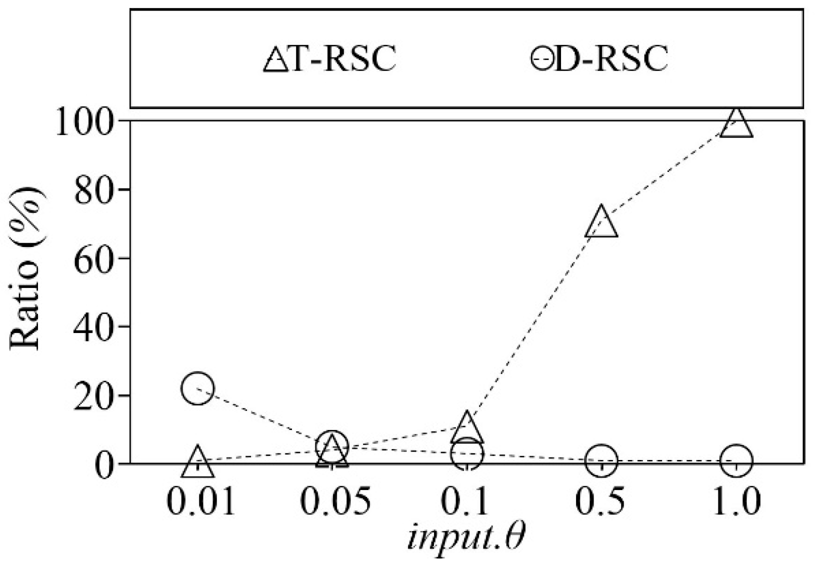
In this experiment, we compare the ratio between the number of diverse and top representative skyline points to the number of overall skyline points |S| with varied input.θ on the anti-correlated synthetic dataset with two dimensions, which contains 600 K data points. Figure 18 shows the ratio between the number of representative skyline points to |S| of both top and diverse representative skyline selection algorithms. The horizontal axis of Figure 18 indicates the input.θ and the vertical axis indicates the ratio of the representative skyline points in percentage. As shown in Figure 18, the ratio between the number of diverse representative skyline points and the number of overall skyline points |S| become smaller than the ratio between the number of top representative skyline points and the number of overall skyline points |S| as the input.θ increases.
The reason behind it is that diverse representative skyline points selection algorithm uses the root to singleton traversal. On the other hand, the top representative skyline points selection algorithm uses the singleton to root traversal. Moreover, depending on the input.θ value, the diverse representative skyline points selection algorithm chooses the representative points of the cluster. In the case of the top representative skyline points selection algorithm, it chooses the skyline points of the cluster with a smaller θ distance than input.θ, which contains the representative point of the root cluster.
4.2.11. Experiment 11. Ratio of the Representative Skyline Points to |S| on Real Dataset with Varied input.θ
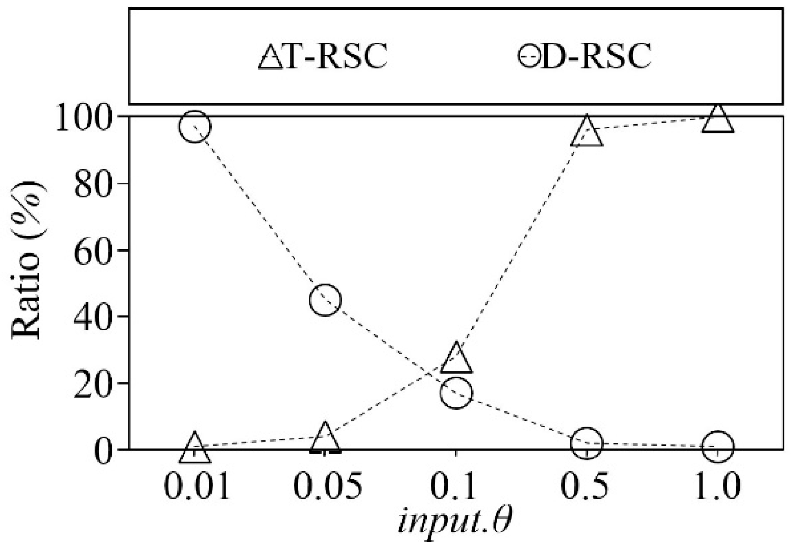
In this experiment, we compare the ratio between the number of diverse and top representative skyline points to the number of overall skyline points |S| with varied input.θ on real NBA dataset. Figure 19 shows the ratio between the number of representative skyline points to |S| of both top and diverse representative skyline selection algorithms. The horizontal axis of Figure 19 indicates the input.θ and the vertical axis indicates the ratio of the representative skyline points in percentage. As shown in Figure 19, the ratio between the number of diverse representative skyline points and the number of overall skyline points |S| and ratio between the number of top representative skyline points and the number of overall skyline points |S| changes drastically as the input.θ increases.
The main reason is the distribution of the NBA dataset. We can assume that the NBA dataset is densely populated. In addition, this sudden change in the ratio occurs because diverse representative skyline points selection algorithm uses root to singleton traversal. On the other hand, the top representative skyline points selection algorithm uses a singleton to root traversal. Moreover, depending on the input.θ value diverse representative skyline points selection algorithm chooses the representative points of the cluster. In the case of the top representative skyline points selection algorithm, it chooses the skyline points of the cluster with a smaller θ distance than input.θ, which contains the representative point of the root cluster.
5. Conclusions
In this paper, we have proposed a novel representative skyline query processing method based on the hierarchical agglomerative clustering method, which solves the problems of the existing methods. With the proposed method, once the hierarchical agglomerative clustering structure is created, changing the global threshold does not trigger the re-computation problem. Because we use centroid linkage to cluster the skyline points, our method shows the exact representatives in any dimension. In addition, we have defined a structure that enables us to obtain a set of top and diverse representative skyline points. This structure makes our method more flexible than the existing methods. Moreover, the representative skyline points found by our proposed method can show the full contour of the overall skyline points.
We have performed extensive experiments on both synthetic and real datasets with varying dimensions, cardinality and attribute correlation. Experimental results have demonstrated that the proposed method is superior compared with the existing state-of-the-art methods in terms of re-computation time consumption and quality of the representation.
As we use a naive method to create the dendrogram, one can argue that the proposed method has a computational overhead and memory inefficiency. Moreover, the proposed method may not be useful in continuous representative skyline query processing due to updating the hierarchical clustering requires recreation of the dendrogram. To solve such problems, in exchange for the quality of representation, we can use dimensionality reduction methods or space-filling curves to reduce the computational overhead of the dendrogram creation. On the other hand, by using the subspace partitioning algorithms to create the dendrogram can be another solution. Thus, in our future work, originating a new novel method of creating the scalable dendrogram from skyline points without the computational overhead is the future enhancement.
Author Contributions
Supervision, A.N.; Writing—review and editing, L.B. and A.N.
Funding
This research was supported by Basic Science Research Program through the National Research Foundation of Korea (NRF) funded by the Ministry of Education (NRF-2017R1D1A3B03035729).
Conflicts of Interest
The authors declare no conflict of interest.
References
- Ihm, S.Y.; Lee, K.E.; Nasridinov, A.; Heo, J.S.; Park, Y.H. Approximate convex skyline: A partitioned layer-based index for efficient processing top-k queries. Knowl. Based Syst. 2014, 61, 13–28. [Google Scholar] [CrossRef]
- Wang, S.; Ooi, B.C.; Tung, A.K.H.; Xu, L. Efficient skyline query processing on peer-to-peer networks. In Proceedings of the 23rd International Conference on Data Engineering (ICDE’07), Istanbul, Turkey, 15–20 April 2007; pp. 1126–1135. [Google Scholar]
- Koizumi, K.; Eades, P.; Hiraki, K.; Inaba, M. BJR-tree: Fast skyline computation algorithm using dominance relation-based tree structure. Int. J. Data Sci. Anal. 2018, 7, 17–34. [Google Scholar] [CrossRef]
- Lin, X.; Yuan, Y.; Zhang, Q.; Zhang, Y. Selecting stars: The k most representative skyline operator. In Proceedings of the 23rd International Conference on Data Engineering (ICDE’07), Istanbul, Turkey, 15–20 April 2007; pp. 86–95. [Google Scholar]
- Tao, Y.; Ding, L.; Lin, X.; Pei, J. Distance-Based Representative Skyline. In Proceedings of the 25th International Conference on Data Engineering (ICDE’09), Shanghai, China, 29 March–2 April 2009; pp. 892–903. [Google Scholar]
- Zhao, F.; Das, G.; Tan, K.L.; Tung, A.K.H. Call to order: A hierarchical browsing approach to eliciting users’ preference. In Proceedings of the 2010 ACM SIGMOD international Conference on Management of Data (SIGMOD’10), Indianapolis, IN, USA, 6–10 June 2010; pp. 27–38. [Google Scholar]
- Borzsony, S.; Kossmann, D.; Stocker, K. The skyline operator. In Proceedings of the 17th International Conference on Data Engineering (ICDE’01), Heidelberg, Germany, 2–6 April 2001; pp. 421–430. [Google Scholar]
- Chomicki, J.; Godfrey, P.; Gryz, J.; Liang, D. Skyline with Presorting: Theory and Optimizations. Intell. Inf. Process. Web Min. 2005, 31, 595–604. [Google Scholar]
- Godfrey, P.; Shipley, R.; Gryz, J. Maximal vector computation in large data sets. In Proceedings of the 31st International Conference on Very Large Data Bases (VLDB’05), Trondheim, Norway, 30 August–2 September 2005; pp. 229–240. [Google Scholar]
- Bartolini, I.; Ciaccia, P.; Patella, M. SaLSa: Computing the skyline without scanning the whole sky. In Proceedings of the 15th ACM International Conference on Information and Knowledge Management (CIKM’06), Arlington, VA, USA, 6–11 November 2006; pp. 405–414. [Google Scholar]
- Vlachou, A.; Doulkeridis, C.; Kotidis, Y. Angle-based space partitioning for efficient parallel skyline computation. In Proceedings of the 2008 ACM SIGMOD International Conference on Management of Data (SIGMOD’08), Vancouver, BC, Canada, 9–12 June 2008; pp. 227–239. [Google Scholar]
- Tan, K.L.; Eng, P.K.; Ooi, B.C. Efficient progressive skyline computation. In Proceedings of the 27th International Conference on Very Large Data bases (VLDB’02), Roma, Italy, 11–14 September 2001; pp. 301–310. [Google Scholar]
- Papadias, D.; Tao, Y.; Fu, G.; Seeger, B. An Optimal and Progressive Algorithm for Skyline Queries. In Proceedings of the 2003 ACM International Conference on Management of Data (SIGMOD’03), San Diego, CA, USA, 9–12 June 2003; pp. 467–478. [Google Scholar]
- Lee, K.C.; Lee, W.C.; Zhen, B.; Li, H.; Tian, Y. Z-SKY: An efficient skyline query processing framework based on Z-order. VLDB J. 2010, 19, 333–362. [Google Scholar] [CrossRef]
- Huang, J.; Ding, D.; Wang, G.; Xin, J. Tuning the Cardinality of Skyline. In Proceedings of the 10th Asia-Pacific Web Conference (APWeb’08) Workshops, Shenyang, China, 26–28 April 2008; pp. 220–231. [Google Scholar]
- Yuan, Y.; Lin, X.; Liu, Q.; Wang, W.; Yu, J.X.; Zhang, Q. Efficient computation of the skyline cube. In Proceedings of the 31st International Conference on Very Large Data Bases (VLDB’05), Trondheim, Norway, 30 August–2 September 2005; pp. 241–252. [Google Scholar]
- Xia, T.; Zhang, D.; Tao, Y. On skylining with flexible dominance relation. In Proceedings of the 24th International Conference on Data Engineering (ICDE’08), Cancun, Mexico, 7–12 April 2008; pp. 1397–1399. [Google Scholar]
- Koltun, V.; Papadimitriou, C.H. Approximately dominating representatives. Theor. Comput. Sci. 2007, 371, 148–154. [Google Scholar] [CrossRef] [Green Version]
- Nanongkai, D.; Sarma, A.D.; Lall, A.; Lipton, R.J.; Xu, J. Regret-minimizing representative databases. Proc. VLDB Endowment 2010, 3, 1114–1124. [Google Scholar] [CrossRef] [Green Version]
- Chen, L.; Wu, J.; Deng, S.; Li, Y. Service recommendation: Similarity-based representative skyline. In Proceedings of the 6th World Congress on Services (SERVICES’10), Miami, FL, USA, 5–10 July 2010; pp. 360–366. [Google Scholar]
- Asudeh, A.; Nazi, A.; Zhang, N.; Das, G. Efficient Computation of Regret-ratio Minimizing Set: A Compact Maxima Representative. In Proceedings of the 2017 ACM International Conference on Management of Data (SIGMOD’17), Chicago, IL, USA, 14–19 May 2017; pp. 821–834. [Google Scholar]
- Magnani, M.; Assent, I.; Mortensen, M.L. Taking the Big Picture: Representative skylines based on significance and diversity. VLDB J. 2014, 23, 795–815. [Google Scholar] [CrossRef]
- Salvador, S.; Chan, P. Determining the number of clusters/segments in hierarchical clustering/segmentation algorithms. In Proceedings of the 16th IEEE International Conference on Tools with Artificial Intelligence (ICTAI’04), Boca Raton, FL, USA, 6–8 November 2004; pp. 576–584. [Google Scholar]
- Kurita, T. An Efficient Agglomerative Clustering Algorithm using a Heap. Pattern Recognit. 1991, 24, 205–209. [Google Scholar] [CrossRef]
Figure 1.
An example of computing skyline points.

Figure 2.
Example of 3 diverse and 3 top representative skyline points.

Figure 3.
Overall process of RSC.

Figure 4.
An example of clustering step.

Figure 5.
An example of diverse representative skyline points selection.

Figure 6.
An example of top representative skyline points selection.

Figure 7.
Working process of LMethod.

Figure 8.
Visualization of the Anisotropic dataset.

Figure 9.
Representative skyline points of Anisotropic dataset.

Figure 10.
Comparison of re-computation time on synthetic dataset (varied d).

Figure 11.
Comparison of re-computation time on synthetic dataset (varied |P|).

Figure 12.
Comparison of diverse representation error on Anisotropic dataset.

Figure 13.
Comparison of diverse representation error on NBA dataset.

Figure 14.
Comparison of top representation error on Anisotropic dataset.

Figure 15.
Comparison of top representation error on NBA dataset.

Figure 16.
Comparison of number of cluster accesses on synthetic dataset.

Figure 17.
Comparison of number of cluster accesses on real dataset.

Figure 18.
Ratio of RSC result on synthetic dataset with varied input.θ.

Figure 19.
Ratio of RSC result on real dataset with varied input.θ.


Table 1.
Analysis of current representative skyline query processing methods.
| Method Name | Re-Computation | Diverse Representative | Top Representative |
|---|---|---|---|
| Max-Dom | √ | - | √ |
| δ-Sky | √ | - | √ |
| ε-Sky | √ | - | √ |
| ADR | √ | √ | - |
| Greedy | √ | √ | - |
| Call-to-Order | √ | - | - |
| SBRSA | √ | √ | - |
| RRMS | - | √ | - |
| Big Picture | √ | √ | - |
Table 2.
Detailed properties of experimental environment.
| Property | Value |
|---|---|
| CPU | 4 x Intel(R) Core(TM) i5-4570 (3.20 GHz) |
| RAM | Samsung PC3-12800 8 GB |
| OS | Ubuntu 16.04.3 LTS |
| HDD | Seageate ATA ST500D 500 GB(7200 RPM) |
Table 3.
Parameter settings.
| Parameter | Value Range | Default Settings |
|---|---|---|
| Dataset cardinality | 200 K, 400 K, 600 K, 800 K, 1 M | 600 K |
| input.θ | 0.01, 0.05, 0.1, 0.5, 1.0 | 0.1 |
| Dataset dimension | 2, 3, 4 | 2 |
| k | 2, 4, 6, 8, 10 | 6 |
© 2019 by the authors. Licensee MDPI, Basel, Switzerland. This article is an open access article distributed under the terms and conditions of the Creative Commons Attribution (CC BY) license (http://creativecommons.org/licenses/by/4.0/).
Share and Cite
MDPI and ACS Style
Battulga, L.; Nasridinov, A. Hierarchical Clustering Approach for Selecting Representative Skylines. Information 2019, 10, 96. https://0-doi-org.brum.beds.ac.uk/10.3390/info10030096
AMA Style
Battulga L, Nasridinov A. Hierarchical Clustering Approach for Selecting Representative Skylines. Information. 2019; 10(3):96. https://0-doi-org.brum.beds.ac.uk/10.3390/info10030096
Chicago/Turabian StyleBattulga, Lkhagvadorj, and Aziz Nasridinov. 2019. "Hierarchical Clustering Approach for Selecting Representative Skylines" Information 10, no. 3: 96. https://0-doi-org.brum.beds.ac.uk/10.3390/info10030096
Note that from the first issue of 2016, this journal uses article numbers instead of page numbers. See further details here.