Article

Performance Investigation of Peak Shrinking and Interpolating the PAPR Reduction Technique for LTE-Advance and 5G Signals

1
School of Electrical and Electronic Engineering, Technological University Dublin (TU Dublin), D08 X622 Dublin, Ireland
2
Department of Electronic Engineering, Maynooth Uiversity, Co. Kildare, W23 F2H6 Maynooth, Ireland
*
Author to whom correspondence should be addressed.
Submission received: 30 October 2019 / Revised: 2 December 2019 / Accepted: 18 December 2019 / Published: 28 December 2019
(This article belongs to the Special Issue Emerging Topics in Wireless Communications for Future Smart Cities)

Abstract

:
Orthogonal frequency division multiplexing (OFDM) has become an indispensable part of waveform generation in wideband digital communication since its first appearance in digital audio broadcasting (DAB) in Europe in 1980s, and it is indeed in use. As has been seen, the OFDM based waveforms work well with time division duplex operation in new radio (NR) systems in 5G systems, supporting delay-sensitive applications, high spectral efficiency, massive multiple input multiple output (MIMO) compatibility, and ever-larger bandwidth signals, which has demonstrated successful commercial implementation for 5G downlinks and uplinks up to 256-QAM modulation schemes. However, the OFDM waveforms suffer from high peak to average power ratio (PAPR), which is not desired by system designers as they want RF power amplifiers (PAs) to operate with high efficiency. Although NR offers some options for maintaining the efficiency and spectral demand, such as cyclic prefix based (CP-OFDM), and discrete Fourier transform spread based (DFT-S-OFDM) schemes, which have limiting effects on PAPR, the PAPR is still as high as 13 dB. This value increases when the bandwidth is increased. Moreover, in LTE-Advance and 5G systems, in order to increase the bandwidth, and data-rate, carrier aggregation technology is used which increases the PAPR the same way that bandwidth increment does; therefore, it is essential to employ PAPR reduction in signal processing stage before passing the signal to PA. In this paper, we investigate the performance of an innovative peak shrinking and interpolation (PSI) technique for reducing peak to average power ratio (PAPR) in orthogonal frequency division multiplexing (OFDM) based signals at waveform generation stage. The main idea behind the PSI technique is to extract high peaks, scale them down, and interpolate them back into the signal. It is shown that PSI technique is a possible candidate for reducing PAPR without compromising on computational complexity, compatible for existing and future telecommunication systems such as 4G, 5G, and beyond. In this paper, the PSI technique is tested with variety of signals in terms of inverse fast Fourier transform (IFFT) length, type of the signal modulation, and applications. Additional work has been carried out to compare the proposed technique with other promising PAPR reduction techniques. This paper further validates the PSI technique through experimental measurement with a power amplifier (PA) test bench and achieves an adjacent channel power ratio (ACPR) of less than –55 dBc. Results showed improvement in output power of PA versus given input power, and furthermore, the error vector magnitude (EVM) of less than 1 % was achieved when comparing of the signal after and before modification by the PSI technique.

1. Introduction

The new 5G wireless networks promise a faster data rate and more reliable service to today’s mobile users. New technologies are being designed by wireless engineers around the world everyday, and many of these new technologies, such as autonomous vehicle, virtual reality, and Internet of Things (IoT), are planing to adapt to the first commercial 5G networks in the early 2020s [1,2,3]. Millimeter-waves (mmWaves), small cells, massive multiple input multiple output (MIMO), full duplex, and beam-forming are main features of 5G systems that seem promising for fulfilling ultra-fast systems in demand [4]. In mm wave frequencies, the 5G NR supports up to 52.6 GHz applications, and this system uses orthogonal frequency division multiplexing (OFDM) for waveform generation [1]. It should be noted that this orthogonality is different from the multiple access schemes which may or may not be orthogonal as seen in orthogonal multiple access (OMA), and non-orthogonal multiple access (NOMA) schemes [4]. Although the orthogonality in multiple access scheme has also increment effect on peak to average power ratio (PAPR) for multiple users [5], in this paper only the PAPR of one user signal waveform is analysed. As, Fourier transform [6,7] plays an essential role in developing OFDM signals, it is fundamental to understand the connection of Fourier transform and creation of high peaks in any multi-carrier signal which has been used in many telecommunication systems [4].

1.1. Fast Fourier Transform; Origin of High Peak to Average Power Ratio or Crest Factor

A block diagram of OFDM is presented in Figure 1, which presents the process of generating orthogonal frequency division multiplexing (OFDM) at the transmitter and the receiver. The orthogonality characteristic is provided by Fourier transform which is applied to signal in form of inverse and discrete as IDFT in transmitter part, and as discrete form as DFT in the receiver part [8]. As result of Fourier transform, there are construction and destruction effects and some signal peaks cancel each other, and some add which creates high peaks in the time domain. The peak to average power ratio (PAPR) parameter for the signal S ( t ) can be calculated by (1).
P A P R d B = 10 log 10 P ( t ) m a x P ( t ) m e a n
where maximum power, or P m a x , and average power, or P m e a n can be measured as:
P m e a n = m e a n ( P ( t ) ) = m e a n ( abs ( S ( t ) ) 2 ) P m a x = m a x ( P ( t ) ) = m a x ( abs ( S ( t ) ) 2 ) ,
where S ( t ) is time domain signal and can be represented as:
S ( t ) = n = 0 N 1 s ( n ) e j 2 π t n N , t = 0 , 1 , , N 1
where N is the transform size or the number of sample points in the data frame, and j = 1 , s ( n ) is the signal in frequency domain.
It should be noted that the block diagram in Figure 1 represents the signal generation for one user only, and it should not be confused with multiple access techniques such as orthogonal frequency multiple access (OFDMA) for 4G techniques, or recently proposed non-orthogonal multiple access (NOMA) techniques for 5G techniques [9]. In practise, as the value measured from Equation (1), is completely random due to its nature, and it varies from 5 dB to 14 dB, for example, in a LTE signal with bandwidth of 512 Mhz; therefore, the probability of accordance of PAPR is considered to compare two signals together. This probability is defined and explained in Section 3.2.

1.2. Previous Peak to Average Power Ratio or Crest Factor Reduction Works

Here we present a summary of the most popular approaches for PAPR reduction in Table 1. In the literature, algorithms addressing PAPR reduction are also known as crest factor reduction (CFR) algorithms. In order to avoid confusion between crest factor (CF), and clipping and filtering (CF); a technique to reduce PAPR, for the remainder of the manuscript, only the phrase PAPR is used.
Among all techniques that are developed to reduce PAPR, a large proportion of the literature is focused on those categories shortlisted in Table 1 (e.g., see [11]). It is observed that clipping based techniques [12], are considered distortion based methods (which means that applying these methods result in out-of-band distortion); however, due to their good performance and simplicity they are considered one of the most practical PAPR reduction techniques [13]. As shown in Figure 2, the original LTE signal when clipped experiences an increase in its adjacent sideband power levels.
Clipping based techniques are developed based on the simple idea of limiting the signal in transmitter to a desired magnitude level without changing the phase [12,14]. As seen in Figure 2, when a sharp clipping technique is applied, about 20 dB distortion is added to the signal which is not desired. The sharp clipping process can be mathematically presented as:
S ( t ) = C R S ( t ) | S ( t ) | , when P ( t ) > C R S ( t ) = S ( t ) , when P ( t ) C R ,
where P ( t ) is time domain power of the LTE signal S ( t ) . C R denotes clipping ratio, and as it can be seen in the example presented in Figure 2, the C R is 0.0015 .
As shown in Figure 3, two stages of Fourier transform are required in order to remove the unwanted distortion added as a result of the sharp clipping process. These stages require extra computations in the system; however, one filter stage is not sufficient as the PAPR can rise. Clipping has to be preformed again, and in turn, more filtering. A number of loops through the clipping and filtering stages are required to have a clipped signal where distortion added to the main spectrum is minimised. An important benefit about this group of techniques is that they do not need to transfer extra information to the receiver to inform about the modification performed on the signal at the transmitter. For many coding based techniques, such as [15,16], SLM [17], or PTS [18,19] based algorithms, the receiver has to be informed about the modifications performed on the signal at the receiver side, and generally, a compensation block has to be added to the receiver side to reverse the process, and this normally effects the symbol error rate (SER), and error vector magnitude (EVM). Moreover, informing the receiver normally involves transmitting extra bits as side information. In 2011, a technique called DSI-SLM technique was developed [20], which is combination of two techniques of dummy sequence insertion (DSI), and the selected mapping (SLM) technique. The block diagram of DSI-SLM technique is presented in Figure 4.
DSI-SLM approach can reduce the PAPR by more than 4 dB; however, in order to achieve that performance the inverse discrete fast Fourier transform (IDFT) can require being implemented approximately 16 times, which in turn is computationally challenging. Moreover, due to the selection of the sequence with minimum PAPR at the right side of the above block diagram, the information about this selection also has to be sent to the receiver. For example, in order to have 16 selections, 4 extra bits have to be sent. Another challenge for implementing DSI-SLM compared to clipping based techniques is the necessity of implementing compensation algorithm in the receiver side. As seen in block diagram of Figure 4, M different phases ( P h . 1 , P h . 2 , …, P h . M ) are multiplied into the signal. The received signal at the receiver has to be divided by the same phase in order to extract the original signal, this means implementing a complex division block at the receiver, which has its own complications, as explained in [21]. There are some works aimed at improving these complications [22,23] and the authors have designed algorithms to avoid transferring extra bits; however, the complexity at the transmitter, and the channel security, remain challenging.

2. The Peak Shrinking and Interpolation (PSI) Technique

Although most of the recent research into PAPR reduction has concentrated on modified SLM and PTS methods, the most practical technique is a combination of clipping and filtering. The goal of of designing peak shrinking and interpolation (PSI) is to have a technique as practical as clipping, and as specific as windowing, an intermediate technique between windowing and clipping techniques. The idea is to simply find problematic peaks in power domain (time domain), extract them, shrink them, and put them back in their place.
A general block diagram for the PSI technique is illustrated in Figure 5. It is seen that first the signal is generated, the PSI technique splits the signal into a number of slices ( N s ), as shown in Figure 5.

2.1. Detection of a Peak and Its Surrounding

The rational behind the idea of splitting the signal into smaller slices, is to enable parallelization of the process, and looking at peaks closely, as the extent of the peaks varies considerably between slices. The zoomed window (the call-out) in Figure 5 shows slides overlapping (in this case by 1 % ), which helps to ensure that a peak point is not being missed by being on the border of a slice. In terms of identification of high peaks, comparison with threshold can be employed which can be considered similar to many other techniques [11]. Another approach for detecting high peaks is to find maximum point of each slice. An example of a particular example slice is shown in Figure 6.
The location of the peak occurring is indicated as P i n d e x . In a similar way, as seen in Algorithm 1, the address or index for second point before and after the high peak on the left side and right side is indicated as L i n d e x and R i n d e x , where L i n d e x = P i n d e x S U R and R i n d e x = P i n d e x + S U R and S U R indicates the surrounding or skirt of a peak. In should be noted that, unlike previous techniques that consider peaks only by the raised point, here, a peak is defined by its surrounding sample values also. As seen in Algorithm 1, peaks and surrounding points are detected. It should be noted that the process of finding peak points indicated by P i n d e x , can be performed in two ways. The first approach is to enforce a threshold value, which is essentially a crest detection technique. This approach results in a matrix containing a number of points, and each point is addressed in terms of surrounding points. The second approach is find the maximum point of each slice, and define the surrounding points. This technique simplifies the initial process; however, it often needs to be repeated as the PAPR is not satisfactory following the shrinking process performed on the detected peak. It can be concluded that there is trade-off between these two techniques, and depending to the hardware requirement, one can be preferred to another, as the enforcing threshold requires a number of bits to store the information of the peak and its surroundings. This study tested 100 instances of randomly generated signals. It was observed that for the first approach the maximum number of peaks found in each slice was 3, and this means 3 × 5 points have to be stored. This can be improved, as mentioned by the second approach, which requires storage for only 5 points; however, it should be noted that the loop might have to be repeated, and this will multiply the involved computational complexity in number of required iterations.
In the process of developing PSI algorithm, it was observed that the dimension of a peak and its surrounding is very important; therefore, the parameter named surrounding region ( S U R ) is defined in order to show the number of points around the main raised point. Simulations were performed for S U R = 4 , 3 , and 2, and it was found out that S U R = 2 was the most suitable value, as it did not add unnecessary complication, and resulted in changes smooth enough in order to satisfy the EVM target, discussed later. This means that two points on the left side of the peak point, and two points on the right side are considered for each peak; therefore, a total of five points are processed. It can be seen in Algorithm 1, that if a peak is very close to the beginning of the slice ( L i n d e x 0 ), then first point of signal in the slice is taken as left border point ( L i n d e x = 1 ). In the example shown in Figure 6, S U R = 2 , and therefore, L i n d e x = P i n d e x 2 , and R i n d e x = P i n d e x + 2 . It can be seen in Algorithm 1, that if the right side border is very close to the end of the slice ( R i n d e x N , the end point of the signal in the slice with address of N is considered for extraction ( R i n d e x = N ). It should be noted that in the cases mentioned, the number of extracted points will be less than five, and when interpolating the processed peak back to the signal, careful addressing should be preformed.
Algorithm 1 Defining the borders of a peak (surrounding borders)
  • S U R 2 ;
  • P i n d e x index of the peak;
  • L i n d e x Left side border;
  • R i n d e x Right side border;
  • if L i n d e x 0 then
  • L i n d e x = 1 ;
  • else
  • L i n d e x = P i n d e x S U R ;
  • end if;
  • if R i n d e x N then
  • R i n d e x P i n d e x + S U R ;
  • else
  • R i n d e x N ;
  • end if;

2.2. Peak Shrinking Process

Once the peak is detected and extracted, the shrinking process can be performed. Equation (5) shows that the shrinking process can be implemented by a multiplication. It should be noted that this multiplication is performed only on five data sample points when S U R = 2 , as number of data points is equal to ( 2 × S U R + 1 ) . Therefore, it does not need a large amount of memory. The shrinking process can be mathematically presented as:
P e a k S h = P e a k 0 × S R ,
where P e a k 0 is the signal before process, S R is the shrinking ratio, and P e a k S h is the resulting shrunk peak. In simulations we may modify the S R , to achieve different results. The shrinking process illustrated in examples in Figure 7a–c is performed with S R = 0.5 . As it is observed from Table 1, when S R = 0.5 , the performance is the best compared to when S R = 0.4 , 0.6 . It should be noted that when S R = 1 , it means that the peak is not shrunk; therefore, the PAPR remains the same. On the other hand, when S R is selected to be very small, this is the equivalent of removing the signal point. In the latter case, the E V M is degraded since there will be a sharp signal discontinuity. This has a similar effect to performing sharp clipping, and requires many filter stages to compensate. As the main aim here is to reduce the complexity of the system, S R is optimised.

2.3. Matching/Smoothing Algorithm in PSI Technique

Figure 7 presents two cases: (1) the case that the shrunk peak does not need smoothing process is presented, where it is seen that D R is 0.001 which is smaller than D m a x . It should be noted that by checking the EVM performance, the suitable value for D m a x is considered to be 0.005 .
Algorithm 2 Matching/smoothing algorithm (performed after the shrinking process)
  • D Absolute distance between power of borders;
  • D L Left side border point distance between peak surrounding and the rest of the signal;
  • D R Right side border point distance between peak surrounding and the rest of the signal;
  • D m a x Maximum value that D can have = 0.005 (normalised power);
  • if D L D m a x then
  •  Border point is shrunk with S R r e v . instead of SR;
  • end if
  • if D R D m a x then
  •  Border point is shrunk with S R r e v . instead of S R ;
  • end if;
For the next case (2) the peak definitely requires smoothing process, as D R is grater than D m a x , and the peak after the smoothing process is seen in Figure 7c.
It should be noted that in some cases, the peak can be found at the very beginning of the slice, or at the very end of signal ( L i n d e x = 0 or R i n d e x = N ). It can be understood that smoothing algorithm does not have access to the adjacent points to perform smoothing correctly, in order to avoid the scenario which happens 5 % of the times when a signal with length of 30 × 10 3 is tested, overlapped slicing, as seen in Figure 5 is recommended, which removes the scenario completely.

3. Performance Analysis of the PSI Technique

3.1. Analysing the Error Vector Magnitude (EVM)

Error vector magnitude (EVM) is a commonly used figure of merit to quantify the performance of a transmitter or receiver. It quantifies to what extent constellation points deviate from their ideal locations. It should be noted that in many works, root square mean (RMS) of EVM is used [25,26,27]; however, here, in order to analyse the worst case, we consider the maximum of EVM in each symbol as:
E V M m a x = 1 K n = 0 K 1 ( I i I m ) 2 + ( Q i Q m ) 2 P m a x × 100 m a x
where I i and Q i are the I and Q of an ideal signal without PSI modification, and I m and Q m are I and Q of a modified signal after being processed with PSI algorithm. Therefore, ( I i I m ) 2 + ( Q i Q m ) 2 is the measured error between the modified I and Q, and the ideal I and Q.
In order to provide a more comprehensive test of the technique, LTE signals were used for experimentation [28]. The E V M for signal processing on the transmitter should be minimised as much as possible. Here, over 100 randomly generated modulated signals with Offset QPSK (OQPSK) were tested and the E V M was measured as presented in Table 2. OFDM signals with various lengths of inverse fast Fourier transform (IFFT) ( K = 512 , 1024 , 2048 , 4096 , and 8192) were tested with different values of R P , and S R , and the E V M m a x in each case was measured and is presented. It was observed that the maximum EVM captured in Scenario 4 when K = 512 , R P = 10 , S R = 0.5 , and N S = 16 , and the E V M m a x had the lowest value in Scenario 6, when K = 2048 , R P = 5 , and S R = 0.5 .
Table 2 presents six scenarios, as in Scenario 1, R P = 5 , S R = 0.5 , N S = 16 ; Scenario 2, R P = 5 , S R = 0.5 , N S = 32 ; Scenario 3, R P = 10 , S R = 0.5 , N S = 16 ; Scenario 4, R P = 10 , S R = 0.5 , N S = 32 ; Scenario 5, R P = 5 , S R = 0.4 , N S = 16 ; and Scenario 6, R P = 10 , S R = 0.6 , N S = 16 .

3.2. PAPR Reduction Performance; Complementary Cumulative Discrete Function (CCDF), and Time Domain Signal Power Peak Reduction

In order to gauge the effectiveness of the proposed techniques, simulations were first carried out in Matlab [29]. When comparing signals with K = 512 , 1024, 4096, and 8192 analytically, it was expected to experience higher PAPR as K was increased. This is due to a higher probability of the presence of high peaks in general. In order to measure this probability the complementary cumulative distribution function (CCDF) was used, which can be represented as:
C C D F = P ( P A P R ( S ( t ) ) P A P R t h ) ,
where P A P R t h is a threshold PAPR, and P denotes the probability. Again, the modulation scheme used in these tests is offset quadrature shift key (OQPSK), and K is varied from 512 to 8192. It should be noted that the LTE toolbox used did not exceed IFFT length of 2048 [26,30]; however, as carrier aggregated signals in LTE-A and 5G technologies had increased IFFT lengths [31,32,33], in order to validate that this scheme is applicable for LTE-A signals and 5G signals, the test was performed for larger IFFT lengths of K = 4096 and 8192. The comparison of the original signal and the signal with PSI applied in the time domain is shown in Figure 8a, and the CCDF plot is presented in Figure 8b, in which the common point to look at the CCDF for performance comparison is at 10 4 . This means that, for example, an original signal with length of K = 1024 is 0.01 % likely to have PAPR of higher than 12 dB. It is shown that this value is reduced to about 7.2 dB by applying the PSI technique. It should be noted that any improvement in CCDF more than 4 dB aligns with IEEE standards [34], and can be considered a useful technique in practice. A full comparison is displayed in Table 3, which shows in case of K = 8192 , the PAPR is reduced by 4.4 dB. This reduction is same as the reduction for K = 4096 , however the point is that by doubling the value of K, the length of IFFT is doubled, and it is directly related to number of carrier aggregations or in other words, the bandwidth in 5G signal. This consistent performance makes PSI a reliable and adaptive technique for high bandwidth applications as seen in LTE-Advanced, and 5G signals.
An analysis is provided in order to demonstrate value of N S can effect the PAPR reduction performance. It is seen in Figure 9a that increasing the value of N S does not necessarily improve the PAPR reduction performance; here, 16 was the value used for N S . Figure 9b shows how PAPR reduction performance is improved by increasing the value of R P . However, it should be noted that the computational complexity is also affected by incremented R P . It was observed that choosing R P = 10 is sufficient to satisfy the rule of thumb minimum 4 dB PAPR reduction performance. When R P = 10 , it means that 10 iterations for the loop presented in Figure 11, are performed to search for peaks and shrink them. This is by means of employing a search for maximum power points. It should be noted that if threshold enforcement is employed instead of search for maximum point, the loop is replaced with iterative shrinking process, which in fact has same effect in terms of computational complexity. It is in Table 2 that changing N S , R P , and S R has a marginal effect on EVM. As observed from results in Figure 10, the SR value plays an important role for PAPR reduction performance. Therefore, furthermore in Section 3.4, the mathematical relationship between PAPR reduction, and the value of SR is modeled as seen in Figure 14.
It can be observed from the plot, and measurements, that when SR is selected about 0.6 and 0.7, the PAPR reduction achieves its optimum performance, which is 3.45 dB for this particular scenario. This simplifies the implementation of PSI as the S R r e v . has also same value of 0.7; therefore, it can be excluded. It should be noted that this analysis was performed in CCDF of 10 1 , and for full CCDF analysis, the reduction at CCDF of 10 4 was considered, which can be seen in Figure 8b.

3.3. Computational Complexity Comparison

As demonstrated in previous sections, simplicity and EVM performance makes the PSI algorithm a practical method. In this section computational complexity of PSI is analysed and compared with previous techniques. Comparison of the proposed technique was first performed with respect to a PAPR reduction technique implemented on an IC [13]. This technique is an implemented version of a clipping technique [12,14,35]. In general, when analysing the computational complexity, the number of additions and number of multiplications are studied. It should be noted that if an algorithm requires complex multiplications, or complex divisions, they all have to be transformed into real multiplications and additions. For example, as mentioned earlier about SLM based techniques [17,20,36], at the receiver, a compensation block including a complex division is required in order to extract the original transmitted signal [37]. The second parameter that plays an important role in implementing a PAPR reduction technique in hardware is the the memory that is required. Here we analyse the number of bits that are required for implementing a technique. By referring to the simplest example of a clipping based technique presented in Figure 3, it is observed that number of multiplications can be measured by the following:
n m u l , C F = n m u l , C l i p p i n g + n m u l , F F T + n m u l , F i l t e r i n g + n m u l , I F F T ,
where n m u l , C l i p p i n g is the number of multiplications needed for clipping; and as seen in Figure 3, it involves peak detection block, the defining threshold block, and at least one if/else for iterating each loop. The number of multiplications required for a filtering process is presented by n m u l , F i l t e r i n g , and number of multiplications required for performing FFT and IFFT processes is indicated by n m u l , F F T , and n m u l , I F F T . For FFT or IFFT, the number of needed multiplications is calculated from the following equation:
n m u l , I F F T = K log k
where n m u l , I F F T = 3072 , and here it is assumed that K = 1024 . It should be noted that for understanding the filtration process, it can be considered a convolution of two signals with same length in domain of frequency. Number of required multiplications for filtration, n m u l , F i l t e r i n g can be calculated by following formula:
n m u l , I F F T = K 2
where here is it assumed that K = 1024 , and therefore, n m u l , F i l t e r i n g = 1048576 .
It is known that for storage of complex numbers, log 2 n bits is required for absolute of each complex number, and log 2 n is required for storing every angle of every complex number. For example, if we assume a complex number with length of n, the number of needed bits is 2 log 2 n , in order to implement it digitally. When K = 1024 , considering the length of each filter, total 2 K log 2 n = 20 , 480 is required in order to implement CF technique. However, for implementing PSI technique, by referring to Figure 5 and Figure 11, the number of needed multiplications, n m u l , P S I can be calculated as:
n m u l , P S I = n m u l , P e a k + n m u l , B o r d e r s + n m u l , E x t r a c t i n g + n m u l , S h r i n k i n g + n m u l , S m o o t h i n g ,
where the n m u l , P e a k is the number of multiplications required for peak detection.
It should be noted that the process of detecting peaks, or enforcing the threshold, is very similar to CF technique. In the PSI technique there is a process for defining the borders, and the number of modifications required to do this process, n m u l , B o a r d e r s is two, which are for indicating the left border, L i n d e x and right border, R i n d e x . However, these pieces of information need to be temporarily stored, and therefore, two bits of memory are occupied. These indexes are replace by every run, so they do not have to be multiplied into the number of iterating loops. The peak extraction process needs n m u l , E x t r a c t i n g number of multiplications which is zero, as it does not require mathematical calculation; however, extracting each peak requires five bits of memory for each peak point and its surrounding points, two points at the left side and two points at the right side. To aid understanding, let us consider the following example, which shows an extracted peak and its surrounding points:
E x t r a c t e d P e a k P o w e r s e t = [ P ( t ) L i n d e x P ( t ) P i n d e x P ( t ) R i n d e x 1 P ( t ) R i n d e x ] = [ P ( t ) 81 P ( t ) 82 P ( t ) 83 P ( t ) 84 P ( t ) 85 ] = [ 0.002 0.018 0.02 0.004 0 ] ,
where P ( t ) indicates the sample point from the power of the signal S ( t ) , which is the square of absolute the signal as:
P ( t ) = | S ( t ) | 2 .
In order to implement the shrinking process itself, the five points are multiplied by a constant value of the shrinking ratio ( S R ); therefore, we see that n m u l , S h r i n k i n g = 5 . For storing the constant value, one bit of memory is occupied. The last algorithm employed in PSI technique is the smoothing, or matching the border points, and this involves two i f / t h e n loops and it is equivalent to two subtractions and two multiplications [24]. It should be noted that in general the total number of bits required for each PSI loop can be represented as:
n b i t , b o r d e r s = 2 b i t s × R P
where number of PSI loops is shown by R P , and by assuming that R P = 10 , number of required bits for PSI loop can be calculated as:
n m u l , B o a r d e r s = 20 b i t s
From (8) to (15), total computational complexity of PSI technique and CF technique can be calculated, and Table 4 presents a comparison in computational complexity among some the most popular CFR techniques. It should be noted that for techniques of PTS [18,38,39,40], SLM based techniques [20,36,41], the set ups of the algorithms are considered in a way that the PAPR reduction performance is comparable with the PSI technique. This means that number of IDFT processed in both mentioned categories, is considered to be 16, and the length of the signal is considered to be 1024, which indicates the number of bts for storing the phases that are multiplied into the input signal [17,41].
It can be seen in Table 4, that the newly developed technique of by two step peak clipping (TPC) [14], which shows 3.5 dB PAPR reduction with moderate EVM performance, has about double the complexity of the conventional CF, since there are two stages of clipping, and therefore, two stages of FIR filters. The outstanding computational complexity of the PSI technique, which is achieved by the idea of eliminating the filtration process, allows PSI to be considered a very good candidate for existing and future systems.

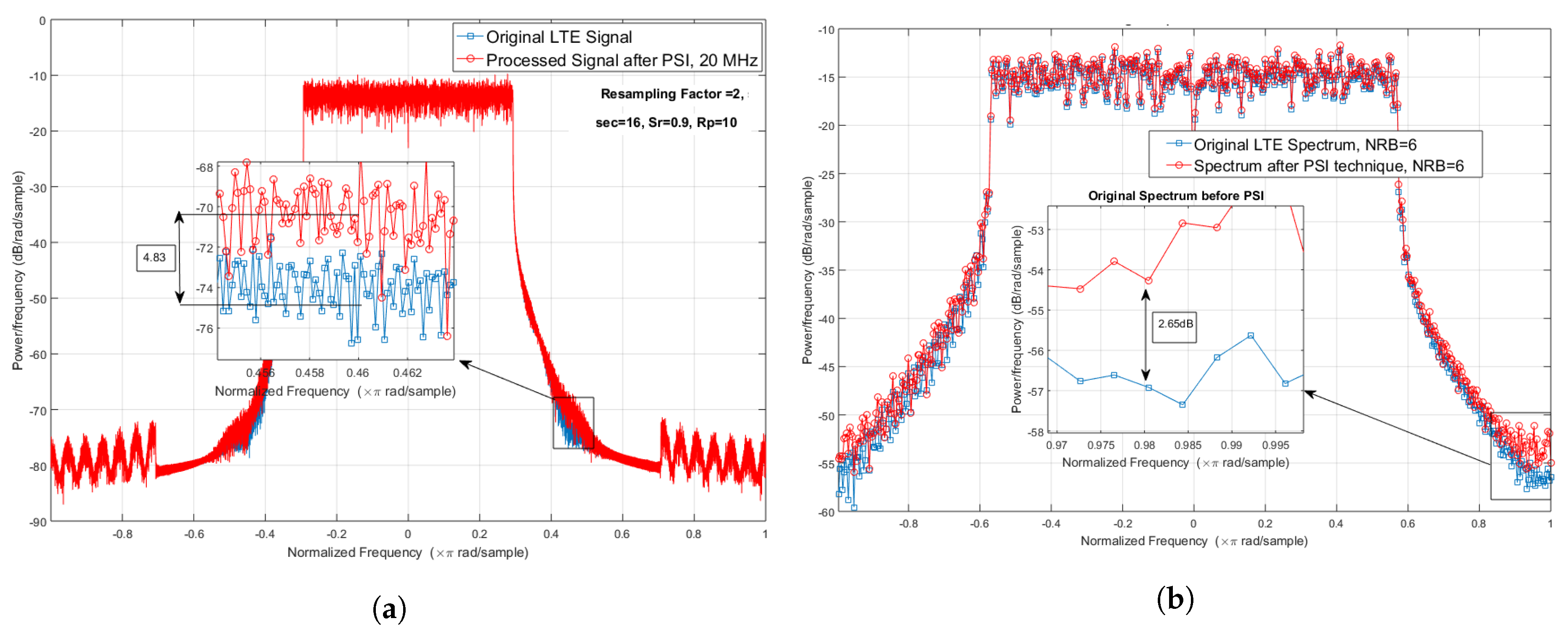
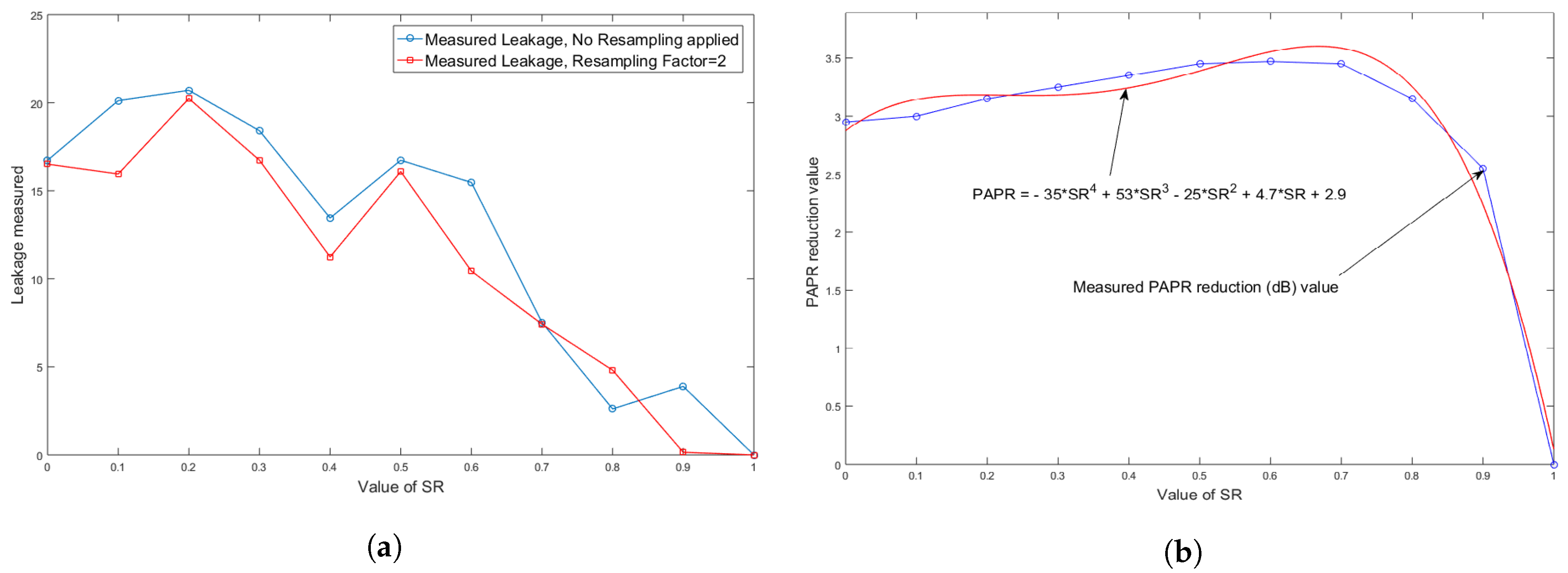
3.4. Signal Spectrum Leakage

As important as it is to analyse a PAPR performance, it should be always considered that by modifying the signal, additional distortion is not added. Here the spectra of the signal with and without PSI technique are compared, and any leakage is carefully measured. This indicates how well the signal is behaving with respect to allocated bandwidth frequency.
Figure 12a represents the spectrum of an LTE signal with a bandwidth of 20 Mhz, and as it is seen there is a slight different between the processed signal and original signal (indicated by red spectrum and blue spectrum in Figure 12 and Figure 13); however, this amount of leakage is normal due to the process of shrinking, and the smoothing algorithm keeps this slight different within acceptable range, as it does not interfere with adjacent channels. However, it should be noted that in case of 5G signals, considering carrier aggregation of for example 20 aggregation process, this leakage should be further tested. Here, the leakage behaviour, as well as PAPR reduction performance are mathematically modeled in order to have good estimation for signals with high bandwidth, and/or carrier aggregation. The PAPR reduction value is formulated as P A P R r e d u c t i o n = 35 S R 4 + 53 S R 3 25 S R 2 + 4.7 S R + 2.9 . Here, a simulation is performed to understand this effect more clearly. The leakage is also measured for variety of values of S R , and it should be noted that in both cases, the re-sampled signal is re-sampled in order to match, The analysis results are presented in Figure 14a,b. As it is observable from Figure 14a, the leakage is reduced by increasing the value of S R . The behaviour is reasonable, as a value of S R shows the amount of shrinking process. The optimum of value observed from other results ( S R o p t ) is sufficient in terms of PAPR reduction, EVM performance, and this leakage. Here, an analysis is presented that explains how PSI technique can be equally used for different types of LTE signal, as described in Table 5. A parameter known as number of resource block (NRB) [30] is varied and the spectrum is compared. The NRB indicates how many blocks of 180 K H z is occupied by the signal structure. The spectrum results in Figure 12a and Figure 13a are captured, when the original and also processed signals are both re-sampled with re-sampling factor of two.
It can be observed that the leakage caused does not reach the next harmony and it is acceptable. Figure 12b and Figure 14b shows the spectrum results when NRB values of 5, and 15 are employed, and the signal is not re-sampled. It should be noted that these tests are performed when N S = 16 , S R = 0.9 , and R P = 10 . Table 5, shows the structure of LTE standard and the PAPR reduction that can be achieved by applying the PSI technique on different settings. It can be seen that when NRB is increased, the length of IFFT is also increased (for instance, when NRB = 6, IFFT/FFT length = 128, and bandwidth is 1.4 ). The PSI technique was tested with all the varieties of signal, and as seen in the Table 5, the spectrum leakage remained small in all cases. It should be noted that here, we consider spectrum leakage very close to the main spectrum in both cases, with and without re-sampling process. The worst case shows about 9.29 dB leakage when NRB is 75. It should be noted that by optimising parameters of the PSI algorithm, such as SR, PR, and NS, the leakage is minimised, as shown in Figure 12a.
However, here in order to have clear picture, worse scenarios were considered. As the variation is comparably small, and close to the main spectrum, this comparison was performed; however, in many works, when the variation and spectrum reshaping is noticeably high, mathematical calculations for adjacent channel power ratio (ACPR) or adjacent channel leakage ratio (ACLR) must be measured. ACPR or ACLR is a measure that shows a ratio between the power of adjacent channel to the main channel’s power. In this paper, the comparison of the modified signal with the original signal without PSI applied are shown with red and blue colours in Figure 12 and Figure 13.
It should be noted that all the tests were performed based on LTE toolbox and QPSK, or OQPSK modulation schemes; however, according to LTE standard documents [28], if test model 3.1 or test model 3.2 are employed, the waveform is slightly different, since the modulation scheme in test model 3.1 is 64 Q A M and the modulation scheme in test model 3.2 is 16 Q A M . PSI was tested with the aforementioned test model signals; by running one test with each, it was found that the original signal with test model 3.1 experiences 12.1859 dB PAPR, and test model 3.2 experiences 16 Q A M PAPR. The PSI technique was able to reduce this PAPR to about 8 dB, which is very similar to QPSK and OQPSK schemes. However, further analysis for EVM for different test models can be performed in future studies.

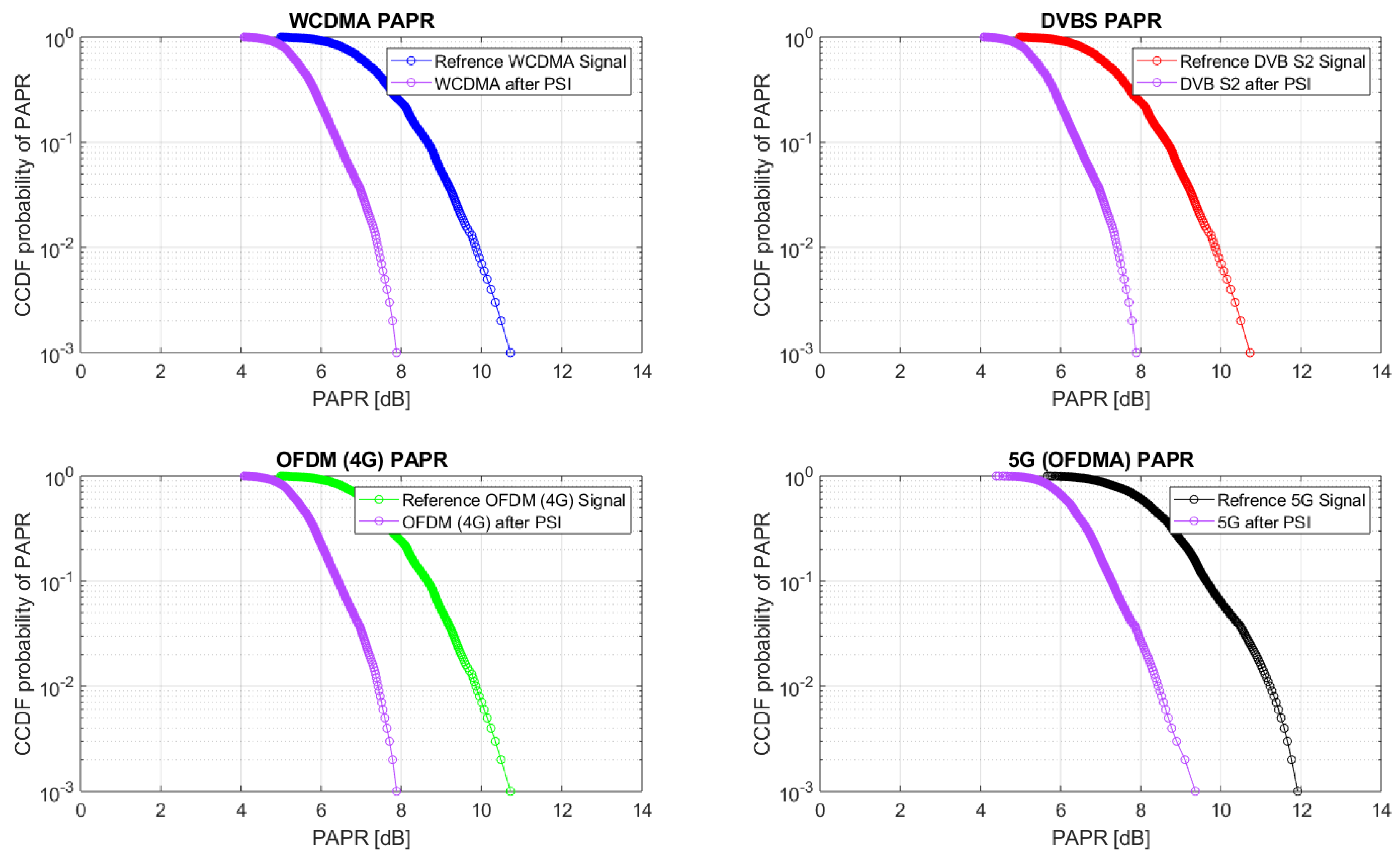
3.5. Testing PSI Performance with WCDMA, DVB S2, 4G, and 5G Signals

Wideband code division multiple access (WCDMA) is one of the earliest signals that experienced high PAPR [43]. Here, a 20 M H Z bandwidth signal was generated and tested with PSI technique. This test was also performed with Digital Video Broadcasting Satellite Second Generation (DVB S2) Signal, a typical 4G orthogonal frequency division multiplexing (OFDM) signal, and a 5G signal based on orthogonal frequency multiplexing division access (OFDMA) signals [44].
The necessity of applying PAPR reduction on DVB S2 signal is due to the need for maximising the power efficiency of amplitude phase shift key (APSK) transmission in satellite channels, as the bandwidth requirements are very limited, and as power efficiency is mostly effected by high power amplifiers (HPAs), and as explained about efficiency section, PAPR determines the efficiency of HPAs in modern signals. Therefore, it is beneficial to show that the PSI technique is usable in the DVB S2 case and for other types of signals. In order to have comparable test, the signals were simulated with close characteristics; for example, length of a inverse fast Fourier transform (IFFT) in three cases of WCDMA, DVB S2, and 4G signals was kept to 2048 in order to fulfil bandwidth of 20 M H Z . It was captured that by testing about 1000 symbols of these signals, the PAPR value fell on about 10.3 dB. As shown in previous test results, this value increases by extending the test to 10 , 000 symbols, as shown in Figure 8b and Figure 10. However, it should be noted that length of IFFT in 5G signals start at 4096, which effects the probability of PAPR value the same way that increasing bandwidth does, and therefore, as seen in Figure 15, the PAPR value of reference 5G signal is about 12 dB at CCDF of 10 3 . The probability of PAPR after the PSI technique is shown by purple colour plots in Figure 15. It is observed that in cases of WCDMA, DVB S2, and 4G signals, PSI reduces the PAPR by about 2.4 dB at CCDF of 10 3 ; it should be noted that this performance increases by looking at CCDF of 10 4 . Here, due to time limitation, the simulation was performed only 1000 times.

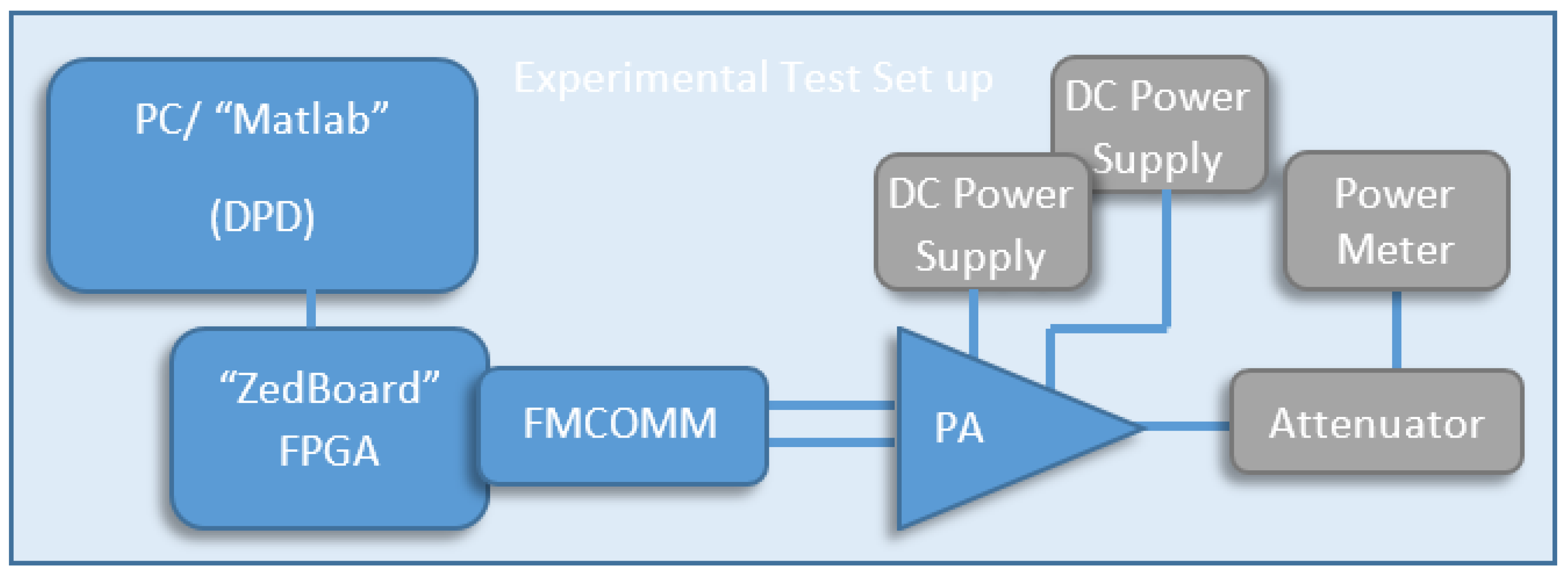
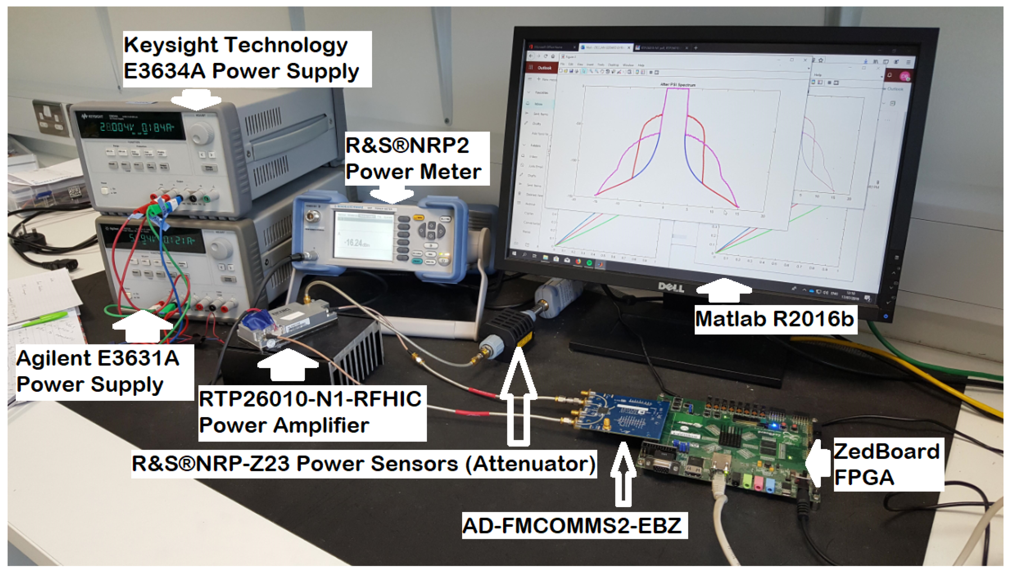
4. Experimental Validation

In this section, an implementation with an FPGA evaluation board is presented. The general implementation set up is shown Figure 16, and laboratory test bench in Figure 17. As seen in this figure, a Zedboard FPGA board (ZedBoard Zynq®-7000 ARM/FPGA SoC Development Board [45]) was connected to a computer running Matlab R2016b simulation tool. This connection can be established using the 10/100/1000 Ethernet port [46]. The Zedboard was connected to an AD-FMCOMMS2-EBZ board [47], which is a FMC board for the AD9361, a highly integrated agile RF transceiver [48]. However, due to the limitation of the instantaneous bandwidth less than or equal to 56 MHz, this limits implementation of DPD, in this experiment to 5 MHz bandwidth signals.
The signal was passed through to the power amplifier (PA). In this work, an RTP26010-N1 RFHIC was used for amplification [49]. This power amplifier from class Doherty [50] has maximum output power of 47 W.
A major component of the experimental validation is to confirm that the PSI technique does not apply additional distortion outside the main channel. As such, it is beneficial to experimentally validate the PSI technique on the bench with a nonlinear PA. Additional DPD linearisation was also applied to the signal in order to linearise the PA output and perform as close a test to a real world scenario as possible. The resulting spectrum and amplitude/amplitude (AM/AM) behaviour of PA was compared with and without DPD, and PSI technique. The DPD linearisation is widely used in many applications, such as cellular telecommunications and satellite linking, because of its relatively simple implementation [51,52,53]. Here a DPD based on the least squares (LS) optimisation technique was used [54]. For simplicity the number of coefficients was minimised; the AM/AM behaviour of PA is plotted in Figure 18b. The inverse of this dynamic nonlinearity was applied to the signal prior passing it through the PA. As mentioned earlier, as DPD relies on the initial response of PA, in order to operate, a wide-bandwidth should be considered; for example, if the signal generated has 5 MHz bandwidth, the bandwidth allowed for FMCOMM and FPGA should be able to compute 5 times that [47]. Therefore, the test signal presented in Figure 18a,b, had a 25 MHz bandwidth. It is seen in Figure 18a, that when a signal is passed through the PA, the distorted output signal has an ACPR or ACLR of approximately 30 dBc. Once DPD is applied, this distortion is reduced to 55 dBc. Applying the PSI to the signal also does not distort the spectrum beyond that of the pre-distorted signal. The PA AM/AM behaviour with and without DPD and PSI are shown, and again, the PSI technique does not impair the overall performance. It is important to note that by applying PSI technique allows the PA has to operate longer in more efficient mode. This can be seen by more frequent data points in the saturation region, as illustrated in the zoomed rectangle frame in Figure 18b. The test presented in Figure 17 and Figure 18a showed that about 1 dB increment in the output of PA was achieved by applying the PSI algorithm.

5. Conclusions

This article is an extension of work on a novel technique presented for PAPR reduction of OFDM based signals at the 2019 Wireless-Days Conference in Manchester [24]. A more than 4 dB PAPR reduction at CCDF of 10 4 or 0.0001 , while the EVM performance degraded by less than 1 % , was demonstrated. In order to explore the practicality of the PSI technique, more evaluations and tests have been performed. The CCDF analysis was tested using LTE signals with IFFT lengths of 4096 and 8192 (in the case of an aggregated signal), with bandwidths of 40 MHz and beyond. Furthermore, the PSI technique was tested with a Doherty PA and a FPGA evaluation board. It was seen that the DPD is able to operate almost in same way as it does without PSI; however, with PSI applied, the PA has more chance to operate in higher power region without experiencing non-linearity. It was observed from experimental tests that the back-off is improved by about 1 dB. Studies showed similar performance for 16 Q A M and 64 Q A M modulation schemes. For future work, generating co-sim block and compiling the algorithm directly on FPGA is recommended; this will indicate the exact amount of hardware resources required for implementing the proposed technique in hardware. It is expected that by optimising all the parameters of PSI algorithm, the output power value achievable can be increased further in future work. Moreover, bit error rate (BER) and symbol error rate (SER) can be investigated in future works.

Author Contributions

Conceptualization, S.M., R.F., D.M., and J.D.; Data curation, S.M., D.M., and J.D.; Funding acquisition, R.F.; Investigation, R.F.; Methodology, S.M.; Resources, R.F., and J.D.; Supervision, R.F., D.M., and J.D.; Validation, S.M., and J.D.; Writing—original draft, S.M.; Review, and editing, S.M., D.M., and J.D. All authors have read and agreed to the published version of the manuscript.

Funding

This publication has emanated from research conducted with the financial support of Science Foundation Ireland (SFI) and was co-funded under the European Regional Development Fund under grant number 13 / R C / 2077 .

Acknowledgments

The help and support of James Kinsella and Joanna O’Grady, are acknowledged and appreciated.

Conflicts of Interest

The authors declare no conflict of interest.

References

  1. Buritica, A. From Waveforms to MIMO: 5 Things for 5G New Radio; National Instruments: Austin, TX, USA, 2019. [Google Scholar]
  2. 5G: New Wave in the IoT Regime. Available online: https://www.microwavejournal.com/articles/ 33187-g-new-wave-in-the-iot-regime (accessed on 21 December 2019).
  3. Opportunities for High Frequency Materials in 5G and the IoT. Microw. J. 2019, 60, 88–96.
  4. Baig, I. A Precoding-Based Multicarrier Non-Orthogonal Multiple Access Scheme for 5G Cellular Networks. IEEE Access 2017, 5, 19233–19238. [Google Scholar] [CrossRef]
  5. Rajasekaran, A.S.; Vameghestahbanati, M.; Farsi, M.; Yanikomeroglu, H.; Saeedi, H. Resource Allocation-Based PAPR Analysis in Uplink SCMA-OFDM Systems. IEEE Access 2019, 7, 162803–162817. [Google Scholar] [CrossRef]
  6. Carslaw, H.S.H.S. Introduction to the Theory of Fourier’s Series and Integrals; Macmillan Publishers Ltd: London, UK, 1921; pp. 1874–1954. [Google Scholar]
  7. Levy, M.M. Fourier transform analysis. J. Br. Inst. Radio Eng. 1946, 6, 228–246. [Google Scholar] [CrossRef]
  8. Mohammady, S.; Sulaiman, N.; Sidek, R.M.; Varahram, P.; Hamidon, M.N. FPGA Implementation of Inverse Fast Fourier Transform in Orthogonal Frequency Division Multiplexing Systems. In Fourier Transform; Salih, S.M., Ed.; IntechOpen: Rijeka, Croatia, 2012; Chapter 6. [Google Scholar] [CrossRef] [Green Version]
  9. Usman, M.R.; Khan, A.; Usman, M.A.; Shin, S.Y. Joint non-orthogonal multiple access (NOMA) Walsh-Hadamard transform: Enhancing the receiver performance. China Commun. 2018, 15, 160–177. [Google Scholar] [CrossRef]
  10. Prasad, R. OFDM for Wireless Communications Systems; Artech House Universal Personal Communications Series; Artech House: London, UK, 2004. [Google Scholar]
  11. Rahmatallah, Y.; Mohan, S. Peak-To-Average Power Ratio Reduction in OFDM Systems: A Survey And Taxonomy. IEEE Commun. Surv. Tutor. 2013, 15, 1567–1592. [Google Scholar] [CrossRef]
  12. May, T.; Rohling, H. Reducing the peak-to-average power ratio in OFDM radio transmission systems. In Proceedings of the VTC ’98, 48th IEEE Vehicular Technology Conference. Pathway to Global Wireless Revolution (Cat. No.98CH36151), Ottawa, ON, Canada, 21–21 May 1998; Volume 3, pp. 2474–2478. [Google Scholar] [CrossRef]
  13. Texas Instruments. GC5328 Datasheet, Low-Power Wideband Digital Predistortion Transmit Processor; Texas Instruments: Dallas, TX, USA, 2009; Available online: http://www.ti.com/lit/ds/slws218a/slws218a.pdf (accessed on 21 December 2019).
  14. Chen, L.; Chen, W.; Liu, Y.; Yang, C.; Feng, Z. An Efficient Directional Modulation Transmitter With Novel Crest Factor Reduction Technique. IEEE Microw. Wirel. Compon. Lett. 2019, 1–3. [Google Scholar] [CrossRef]
  15. Jones, A.E.; Wilkinson, T.A.; Barton, S.K. Block coding scheme for reduction of peak to mean envelope power ratio of multicarrier transmission schemes. Electron. Lett. 1994, 30, 2098–2099. [Google Scholar] [CrossRef]
  16. Kwon, J.W.; Park, S.K.; Kim, Y. Peak-to-average power ratio reduction by the partial shift sequence method for space-frequency block coded OFDM systems. In Proceedings of the 2009 IEEE International Conference on Network Infrastructure and Digital Content, Beijing, China, 6 November 2009; pp. 890–893. [Google Scholar] [CrossRef]
  17. Varahram, P.; Ali, B. Peak to Average Power Ratio Reduction Based on Optimum Phase Sequence in Orthogonal Frequency Division Multiplexing Systems. In Advanced Transmission Techniques in WiMAX; Hincapie, R., Sierra, J.E., Eds.; IntechOpen: London, UK, 2012; pp. 217–238. [Google Scholar]
  18. Varahram, P.; Al-Azzo, W.F.; Ali, B.M. A low complexity partial transmit sequence scheme by use of dummy signals for PAPR reduction in OFDM systems. IEEE Trans. Consum. Electron. 2010, 56, 2416–2420. [Google Scholar] [CrossRef]
  19. Varahram, P.; Ali, B.M.; Al-Azzo, W. Low complexity ADRG-PTS scheme for PAPR reduction in OFDM systems. In Proceedings of the 13th International Conference on Advanced Communication Technology (ICACT2011), Gangwon-Do, South Korea, 13–16 February 2011; pp. 331–334. [Google Scholar]
  20. Mohammady, S.; Sidek, R.M.; Varahram, P.; Hamidon, M.N.; Sulaiman, N. A new DSI-SLM method for PAPR reduction in OFDM systems. In Proceedings of the 2011 IEEE International Conference on Consumer Electronics (ICCE), Berlin, Germany, 6–8 Spetember 2011; pp. 369–370. [Google Scholar] [CrossRef]
  21. Mohammady, S.; Sulaiman, N.; Sidek, R.; Varahram, P.; Hamidon, M.N. FPGA Implementation of Inverse Fast Fourier Transform in Orthogonal Frequency Division Multiplexing Systems; Intech Open Limited: London, UK, 2012. [Google Scholar]
  22. Razavi, S.; Sulaiman, N.; Sidek, R.M.; Mohammady, S.; Varahram, P. Analysis on the parameters of selected mapping without side information on PAPR performances. In Proceedings of the 2014 IEEE 5th Control and System Graduate Research Colloquium, Shah Alam, Malaysia, 4–5 August 2014; pp. 43–46. [Google Scholar] [CrossRef]
  23. Razavi, S.; Sulaiman, N.; Mohammady, S.; Sidek, R.M.; Varahram, P. Efficiency analysis of PAPR reduction schemes. In Proceedings of the 2012 International Symposium on Telecommunication Technologies, Kuala Lumpur, Malaysia, 26–28 November 2012; pp. 279–284. [Google Scholar] [CrossRef]
  24. Mohammady, S.; Farrell, R.; Malone, D.; Dooley, J. Peak Shrinking and Interpolating Technique for reducing Peak to Average Power Ratio. Wirel. Days (WD) 2019, 1–6. [Google Scholar] [CrossRef] [Green Version]
  25. Kotzer, I.; Har-Nevo, S.; Sodin, S.; Litsyn, S. An Analytical Approach to the Calculation of EVM in Clipped Multi-Carrier Signals. IEEE Trans. Commun. 2012, 60, 1371–1380. [Google Scholar] [CrossRef]
  26. Muntean, V.H.; Otesteanu, M. WiMAX versus LTE—An overview of technical aspects for next generation networks technologies. In Proceedings of the 2010 9th International Symposium on Electronics and Telecommunications, Timisoara, Romania, 11–12 November 2010; pp. 225–228. [Google Scholar] [CrossRef]
  27. Liu, Q.; Baxley, R.J.; Ma, X.; Zhou, G.T. Error vector magnitude optimization for OFDM systems with a deterministic peak-to-average power ratio constraint. In Proceedings of the 2008 42nd Annual Conference on Information Sciences and Systems, Princeton, NJ, USA, 19–21 March 2008; pp. 101–104. [Google Scholar] [CrossRef]
  28. ETSI Standards. LTE Evolved Universal Terrestrial Radio Access (E-UTRA) Base Station (BS) Radio Transmission and Reception (3GPP TS 36.104 Version 13.7.0 Release 13). 2017. Available online: https://www.etsi.org/deliver/etsi_tr/101400_101499/101477/01.01.01_60/tr_101477v010101p.pdf (accessed on 21 December 2019).
  29. LTE Tool Box in Matlab. The Mathworks, USA. Available online: https://uk.mathworks.com/products/lte.html?requestedDomain= (accessed on 21 December 2019).
  30. Rémy, J.; Letamendia, C. LTE Standards; Iste Series; Wiley: Hoboken, NJ, USA, 2014. [Google Scholar]
  31. Tsai, W.; Liou, C.; Peng, Z.; Mao, S. Wide-Bandwidth and High-Linearity Envelope- Tracking Front-End Module for LTE-A Carrier Aggregation Applications. IEEE Trans. Microw. Theory Tech. 2017, 65, 4657–4668. [Google Scholar] [CrossRef]
  32. Lu, F.; Xu, M.; Cheng, L.; Wang, J.; Shen, S.; Zhang, J.; Chang, G. Sub-Band Pre-Distortion for PAPR Reduction in Spectral Efficient 5G Mobile Fronthaul. IEEE Photonics Technol. Lett. 2017, 29, 122–125. [Google Scholar] [CrossRef]
  33. 5G. 5G vs 4G: No Contest. Available online: https://5g.co.uk/guides/4g-versus-5g-what-will-the-next-generation-bring/ (accessed on 21 December 2019).
  34. IEEE Standards, USA. IEEE 802.16e WiMAX OFDMA Signal Measurements and Troubleshootin; Agilent Application Note 1578; IEEE Standards: Piscataway, NJ, USA, 2011. [Google Scholar]
  35. Wang, Y.; Luo, Z. Optimized Iterative Clipping and Filtering for PAPR Reduction of OFDM Signals. IEEE Trans. Commun. 2011, 59, 33–37. [Google Scholar] [CrossRef]
  36. Bauml, R.W.; Fischer, R.F.H.; Huber, J.B. Reducing the peak-to-average power ratio of multicarrier modulation by selected mapping. Electron. Lett. 1996, 32, 2056–2057. [Google Scholar] [CrossRef] [Green Version]
  37. Mohammady, S.; Varahram, P.; Sidek, R.; Hamidon, M.N.; Sulaiman, N. FPGA Implementation of the Complex Division in Digital Predistortion Linearizer. Aust. J. Basic Appl. Sci. (AJBAS) 2010, 5028–5037. [Google Scholar] [CrossRef]
  38. Muller, S.H.; Huber, J.B. OFDM with reduced peak-to-average power ratio by optimum combination of partial transmit sequences. Electron. Lett. 1997, 33, 368–369. [Google Scholar] [CrossRef] [Green Version]
  39. Muller, S.H.; Huber, J.B. A novel peak power reduction scheme for OFDM. In Proceedings of the 8th International Symposium on Personal, Indoor and Mobile Radio Communications—PIMRC ’97, Helsinki, Finland, 1–4 September 1997; Volume 3, pp. 1090–1094. [Google Scholar] [CrossRef]
  40. Jawhar, Y.A.; Audah, L.; Taher, M.A.; Ramli, K.N.; Shah, N.S.M.; Musa, M.; Ahmed, M.S. A Review of Partial Transmit Sequence for PAPR Reduction in the OFDM Systems. IEEE Access 2019, 7, 18021–18041. [Google Scholar] [CrossRef]
  41. Mohammady, S.; Sulaiman, N.; Varahram, P.; Sidek, R.M.; Hamidon, M.N. Performance investigation between DSI-SLM and DSI-PTS schemes in OFDM signals. In Proceedings of the 2012 International Symposium on Telecommunication Technologies, Sarajevo, Bosnia Herzegovina, 25–27 October 2012; pp. 210–214. [Google Scholar] [CrossRef]
  42. Rohde Schwarz 5G Poster: Be ahead in 5G. Demystifying 5G NR. Available online: https://www.mobilewirelesstesting.com/wp-content/uploads/2018/05/5GNR-IO_Rohde-Schwarz_April-2018-Blasts.pdf (accessed on 21 December 2019).
  43. Lashkarian, N.; Tarn, H.; Dick, C. Crest Factor Reduction in Multi-carrier WCDMA Transmitters. In Proceedings of the 2005 IEEE 16th International Symposium on Personal, Indoor and Mobile Radio Communications, Berlin, Germany, 11–14 September 2005; Volume 1, pp. 321–325. [Google Scholar] [CrossRef]
  44. Mohammady, S.; Varahram, P. Introductory Chapter: Multiplexing History—How It Applies to Current Technologies. In Multiplexing; Mohammady, S., Ed.; IntechOpen: Rijeka, Croatia, 2019; Chapter 1. [Google Scholar] [CrossRef] [Green Version]
  45. Digilent ZedBoard Zynq®-7000 ARM/FPGA SoC Development Board. Available online: https://www.xilinx.com/products/boards-and-kits/1-elhabt.html.html (accessed on 21 December 2019).
  46. Digilentinc Zedboard Schematic. Available online: www.Zedboard.org (accessed on 21 December 2019).
  47. AD-FMCOMMS2-EBZ User Guide. Available online: https://wiki.analog.com/resources/eval/ user-guides/ad-fmcomms2-ebz (accessed on 21 December 2019).
  48. Analog Devices AD9361 Integrated Radio Frequency (RF) Agile Transceiver. Available online: https://www.analog.com/en/products/ad9361.html (accessed on 21 December 2019).
  49. GaN-SiC Pallet Amplifier RTP26010-N1. Available online: https://dtsheet.com/doc/841692/rfhic-rtp26010-n1 (accessed on 21 December 2019).
  50. Doherty, W.H. A New High Efficiency Power Amplifier for Modulated Waves. Proc. Inst. Radio Eng. 1936, 24, 1163–1182. [Google Scholar] [CrossRef]
  51. Mohammady, S.; Sidek, R.M.; Varahram, P.; Hamidon, M.N.; Sulaiman, N. A low complexity selected mapping scheme for peak to average power ratio reduction with digital predistortion in OFDM systems. Int. J. Commun. Syst. 2013, 26, 481–494. [Google Scholar] [CrossRef]
  52. Cheang, C.; Mak, P.; Martins, R.P. A Hardware-Efficient Feedback Polynomial Topology for DPD Linearization of Power Amplifiers: Theory and FPGA Validation. IEEE Trans. Circ. Syst. I Regul. Pap. 2018, 65, 2889–2902. [Google Scholar] [CrossRef]
  53. Prata, A.; Santos, J.C.; Oliveira, A.S.R.; Borges Carvalho, N. Agile All-Digital DPD Feedback Loop. IEEE Trans. Microw. Theory Tech. 2017, 65, 2476–2484. [Google Scholar] [CrossRef]
  54. Byrne, D.; Farrell, R.; Madhuwantha, S.; Leeser, M.; Dooley, J. Digital Pre-distortion Implemented Using FPGA. In Proceedings of the 2018 28th International Conference on Field Programmable Logic and Applications (FPL), Dublin, Ireland, 27–31 August 2018; pp. 453–4531. [Google Scholar] [CrossRef]
Figure 1. Block diagram of orthogonal frequency division multiplexing (OFDM) transmission [10].
Information 11 00020 g001
Figure 2. LTE signal spectrum with/without clipping technique (a); time domain LTE Signal with/without clipping technique (b).
Information 11 00020 g002
Figure 3. Example of conventional clipping and filtering technique.
Information 11 00020 g003
Figure 4. DSI-SLM PAPR reduction technique [20].
Information 11 00020 g004
Figure 5. Block diagram of proposed PSI technique [24].
Information 11 00020 g005
Figure 6. An example of a slice including a high peak.
Information 11 00020 g006
Figure 7. (a) An example of a peak border does not need matching/smoothing; (b) an example of a peak border that needs matching/smoothing; (c) an example of a peak border after the matching/smoothing process [24].
Information 11 00020 g007
Figure 8. (a) Signal power before and after PSI technique [24]. (b) CCDF probability of PAPR before and after PSI technique for K = 1024 , to K = 8192 [24].
Information 11 00020 g008
Figure 9. (a) PAPR reduction performance variation with N S [24]; (b) PAPR reduction performance variation with R P [24].
Information 11 00020 g009
Figure 10. CCDF result versus SR value.
Information 11 00020 g010
Figure 11. The PSI algorithm iteration loop block diagram [24].
Information 11 00020 g011
Figure 12. (a) Signal spectrum before and after PSI technique, when NRB = 100 [24]. (b) Signal spectrum before and after PSI technique for LTE when NRB = 6.
Information 11 00020 g012
Figure 13. (a) Signal spectrum SR = 0.7, NRB = 25 and re-sampling Factor = 2. (b) Signal spectrum when SR = 0.7 and NRB = 25.
Information 11 00020 g013
Figure 14. (a) Leakage behaviour versus SR. (b) PAPR reduction versus SR, and mathematical modelling.
Information 11 00020 g014
Figure 15. CCDF of PAPR reduction performance of PSI technique on multi signals.
Information 11 00020 g015
Figure 16. PA and DPD test diagram.
Information 11 00020 g016
Figure 17. FPGA laboratory test bench set up.
Information 11 00020 g017
Figure 18. (a) Spectrum of PA output signal with and without DPD, and PSI technique (FPGA test). (b) PA AMAM characteristic with and without DPD, and PSI technique (FPGA test).
Information 11 00020 g018
Table 1. Review of common peak to average power ratio (PAPR) reduction techniques.
TechniqueData RateDistortion-lessTransmitterReceiverSide Info.PAPR
(CFR)Loss ComplexityComplexityBitsReduction
Clipping basedNoNoLowLowNoHigh
Coding basedYesYesHighHighNoMedium
PTS basedYesYesHighLowYesHigh
SLM basedNoYesHighLowYesHigh
DSI basedYesYesLowLowNoWeak
Table 2. Maximum measured error vector magnitude (EVM) ( E V M m a x ) for PSI algorithm.
Length of the IFFT (K)Scenario 1Scenario 2Scenario 3Scenario 4Scenario 5Scenario 6
5120.1652%0.1652%0.2035%0.2405%0.2192%0.1857%
10240.0756%0.0756%0.0932%0.1143%0.1053%0.0840%
20480.0345%0.0345%0.0435%0.0542%0.0486%0.0381%
40960.0142%0.0169%0.0189%0.0237%0.0162%0.0156%
81920.0064%0.0083%0.0077%0.0105%0.0079%0.0070%
Table 3. PAPR reduction performance for different length of IFFT at 0.0001 CCDF.
Length of IFFT (K)Original Signal without CFRAfter PSIAmount of Reduction (dB)
102412 dB 7.3 dB 4.7 dB
2048 12.4 dB 7.7 dB 4.7 dB
4096 12.7 dB 8.3 dB 4.4 dB
8192 12.9 dB 8.5 dB 4.4 dB
Table 4. Computational complexity comparison.
Type of CFR TechniqueNumber of Required MultiplicationsNumber of Required Bits
Length of the IFFT ( K = 1024 ) ( n mul ) ( n bit )
Clipping and Filtering (CF) 10 6 10 3
Two Step Peak Clipping (TPC) [14] 2 × 10 6 10 3
DSI-SLM technique [20]478101024
DSI-PTS technique [41]67,112,6151024
Conventional SLM(C-SLM) technique [36] 95 , 620 1024
Peak Shrinking and Interpolation (PSI)144080
Table 5. LTE Signal structure [30,42].
LTENumber ofSignalLTESpectrumSpectrum
WindowingResource BlocksBandwidthIFFT/FFTLeakageLeakage
Size(NRB)(MHz)Size(No Re-Sampling)(Re-Sampling Factor = 2)
461.41281.160.94
61532560.220.08
425551200
6501010244.834.14
8751520483.669.29
81002020486.987.44

