Optimal Feature Aggregation and Combination for Two-Dimensional Ensemble Feature Selection

Abstract

Feature selection is a way of reducing the features of data such that, when the classification algorithm runs, it produces better accuracy. In general, conventional feature selection is quite unstable when faced with changing data characteristics. It would be inefficient to implement individual feature selection in some cases. Ensemble feature selection exists to overcome this problem. However, with the advantages of ensemble feature selection, some issues like stability, threshold, and feature aggregation still need to be overcome. We propose a new framework to deal with stability and feature aggregation. We also used an automatic threshold to see whether it was efficient or not; the results showed that the proposed method always produces the best performance in both accuracy and feature reduction. The accuracy comparison between the proposed method and other methods was 0.5–14% and reduced more features than other methods by 50%. The stability of the proposed method was also excellent, with an average of 0.9. However, when we applied the automatic threshold, there was no beneficial improvement compared to without an automatic threshold. Overall, the proposed method presented excellent performance compared to previous work and standard ReliefF.

1. Introduction

Feature selection is a way of reducing the dimensions/features of data such that, when the classification algorithm runs, it produces better accuracy. The common thing to do is to recognize the domain of the data and to form a set of more relevant features. However, as the amount of data increases, it becomes exhausting to sort relevant features manually. There are several benefits of feature selection, i.e., facilitating data visualization and data understanding, reducing computing time and data storage, and reducing overfitting due to the phenomenon of the curse of dimensionality and improving the performance [1].

There are many ways of building feature selection algorithms, but most feature selection algorithms are categorized into three types. Filter types use feature rank to determine the relevance of each feature [2,3,4,5,6,7,8]. Feature rank is obtained by calculating the correlation between each feature and its predictor class. Consequently, this type has a minimum of computational time. The second type is the wrapper. In this type, a classification algorithm used to determine the most relevant features, which are obtained by looking at the results of the classification algorithm [9,10,11,12]. In line with the wrapper type, the embedded type also uses a classification algorithm to determine the relevant features. The difference is that the feature selection algorithm is embedded in the classification algorithm, such as decision tree, random forest, and neural network [13,14,15].

There were many researches on feature selection in recent years. The research focused on how to optimize the feature selection algorithm. Some used the addition of optimization algorithm [16,17,18,19,20], i.e., genetic algorithm or particle swarm optimization, while some used the fuzzy approach [21,22,23,24,25] and, most recently, the ensemble approach [17,21,26,27,28,29,30,31,32,33]. In general, a conventional feature selection is quite unstable when faced with changing data characteristics. Well, mostly, each algorithm is applied to different cases. Therefore, it would be inefficient to implement a conventional feature selection in some cases, especially when it concerns big data. Ensemble feature selection exists to overcome this problem. With a reasonably simple approach like an ensemble classification, according to Pardo et al. [27], there are two categories, namely, homogeneous and heterogeneous.

Ensemble feature selection can reduce computing time and improve accuracy. The concept of ensemble feature selection is to divide the feature search space of the data into several subsets so as to reduce the complexity of the algorithm. At the end, each subset is combined to get the full results. However, with these advantages, some problems need to be overcome. Bolón–Canedo and Alonso–Betanzos [28] mentioned that some of the problems with ensemble feature selection are as follows:

• Optimal number of ensembles: because the basis of an ensemble is a partition, it is necessary to know the optimal number of partitions. Our research [32] on ensemble feature selection showed that five partitions are better than three and seven.
• Stability of feature selection: this relates to how well the ensemble feature selection produces the same selected features each time.
• Scalability: a conventional feature selection is less efficient in handling big data problems. Logically, ensemble feature selection can handle this problem because of the partition.
• Threshold for rankers: the problem of each feature selection algorithm that uses a filter approach is determining the threshold for the ranker. This threshold determines the number of reduced features.
• Feature aggregation: this problem is related to how to combine features from each subset in the ensemble to produce the most relevant features.
• Explainability: the main problem faced by each algorithm beyond feature selection is clarity of the results obtained. Researchers usually use two approaches, i.e., mathematical proofing or empirical proofing.

Our previous research [32], which focused on how to improve accuracy and computational time, still had a few limitations. The first involved how to calculate the stability of the ensemble feature. The second involved the determination of the threshold for the ranker. The third involved how to aggregate the subsets of features to produce the best result. The focus of this research is creating a new framework that can overcome the problems of stability, threshold, and aggregation of features.

The organization of this paper is as follows: Section 2 describes the dataset, evaluation measurement, and the proposed technique. Section 3 displays the results obtained from several experiments and contains a discussion of the results obtained. Finally, Section 4 concludes the paper.

2. Materials and Methods

2.1. Resources

In this research, an experiment was carried out using a Hewlett-Packard Laptop with an Intel (R) Core (TM) Processor i5-7200U central processing unit (CPU) @ 2.50 GHz, 2712 MHz, with two cores and four logical processors with 8 GB of random-access memory (RAM). This research used MATLAB with several libraries included.

2.2. Dataset

The dataset used in this research was taken from three sources: UCI Machine Learning Repository, Arizona State University feature selection dataset, NIPS 2003 challenge dataset, and Vanderbilt University’s gene expression dataset. There were 14 different datasets with multivariate characteristics and no missing data. These datasets were chosen based on differences in the number of samples, features, and classes, as well as because the datasets had different fields of knowledge. There are three categories or fields of knowledge, for example, artificial data, image data, and medical record data. The aim was to see whether the proposed method could overcome variations of these characteristics.

Table 1. Datasets.

No	Datasets	Categories	# of Samples	# of Features	# of Classes	Source
1	MADELON	Artificial data	2600	500	2	[34]
2	COIL20	Image data	1440	1024	20	[35]
3	GISETTE		7000	5000	2	[34]
4	USPS		9298	256	10	[35]
5	YALE		165	1024	15	[35]
6	ORL		400	1024	40	[35]
7	CTG	Medical record data	2126	23	3	[36]
8	11-TUMORS		174	12,533	11	[37]
9	LUNG CANCER		203	12,600	5	[37]
10	TOX_171		171	5748	4	[35]
11	PROSTATE_GE		102	5966	2	[35]
12	GLI_85		85	22,283	2	[35]
13	LYMPHOMA		96	4026	9	[35]
14	SMK_CAN_187		187	19,993	2	[35]

shows the characteristics of the datasets and their sources.

2.2.1. Artificial Data

MADELON is an artificial dataset consisting of 32 clusters. MADELON has five hypercube dimensions (an analog n-dimensional square and cube) and is labeled +1 and −1 at random. Five dimensions represent the five informative features. Then, out of the five features, 15 additional combinations are made to produce a total of 20 informative and redundant sets of features. The sequence of features and patterns in this dataset is randomized. MADELON is also one of five datasets in NIPS 2003.

2.2.2. Image Data

In this research, the proposed method was tested on five image datasets with different criteria, one of which was the number of classes. The first dataset was the Columbia University Image Library (COIL20). COIL 20 is a face image dataset consisting of 20 objects. Each object has 72 images that were taken five degrees apart when the object rotated on a turntable. The size of each image is 32 × 32 pixels, represented by a 1024-dimensional vector.

The second data was GISETTE. GISETTE is a handwritten number recognition dataset. The problem involves differentiating between numbers four and nine. The data are processed in such a way (normalized and centered) leading to a fixed size of 28 × 28. The sequence of features and patterns in this dataset is randomized, where information from the features is not provided to avoid bias in the feature selection process. GISETTE is one of five datasets in NIPS 2003.

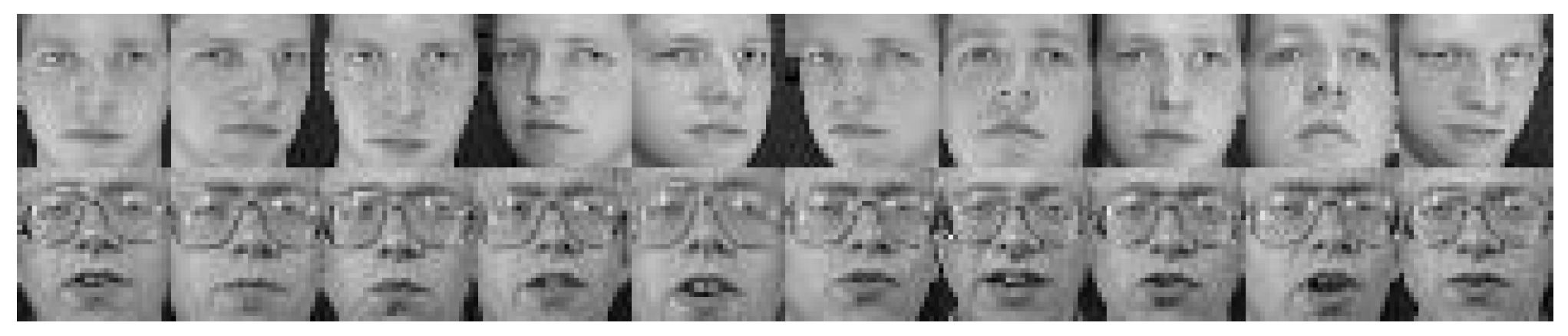
The third dataset was USPS. USPS is also a digit handwritten dataset. It is similar to GISETTE, but the digits used in USPS are all digits from 0–9. The digits are converted to a 16 × 16 image. Figure 1 shows sample images from the USPS dataset.

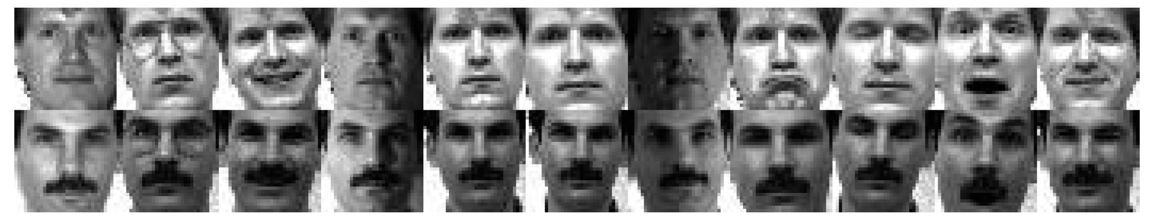
The fourth dataset was YALE. YALE is a face image dataset from 15 individuals. Each individual has 11 image variations, which are center-light, with glasses, happy, left-light, without glasses, normal, right-light, sad, sleepy, surprised, and winking. The total dataset includes 165 grayscale images in GIF format. Figure 2 shows sample images from the YALE dataset.

Similar to YALE, ORL is also a face image dataset. ORL contains 10 different images each of 40 distinct subjects. The images were taken several times, varying the illumination, facial looks (open/closed eyes), facial emotions (smiling/not smiling), and facial appearances (glasses/no glasses). The images were taken against a dark background with the subjects facing the camera (with tolerance for some side movement). Figure 3 shows sample images from the ORL dataset.

2.2.3. Medical Record Data

The proposed method was also tested using medical record datasets. There were six datasets tested, five of which were gene expression datasets. The first one was a cardiotocography (CTG) dataset. CTG includes medical record data for fetal heart rate and uterus contraction. CTG measures the fetal heart rate and, at the same time, monitors contractions in the uterus (uterus). CTG is different from an electrocardiogram (ECG). An ECG detects the heart rate by measuring the electrical activity produced by the heart during contractions. CTG uses ultrasound waves called Doppler waves to measure fetal movements. The way it works is by sending ultrasound waves into the mother’s body; then, when it hits the fetus, the ultrasound waves bounce back with varying strength. The bouncing waves are measured as the fetal heart rate. Contractions can be measured using the tocodynamometer found on CTG. The tocodynamometer measures the tension in the mother’s abdominal wall.

The 11-TUMORS dataset was from the Gene Expression Model Selector. The 11-TUMORS consists of 11 types of tumors in humans placed in a microarray. The 11 classes in this dataset included prostate, bladder/ureter, breast, colorectal, gastroesophageal, kidney, liver, ovary, and pancreatic cancer, as well as lung adenocarcinoma and lung squamous cell carcinoma.

LUNG CANCER was a dataset from the Gene Expression Model Selector. This dataset consisted of four types of lung cancer and normal samples. The total data is 203 specimens with 186 lung tumors and 17 healthy lung specimens. Of these, 125 adenocarcinoma samples were associated with clinical data and with histological slides from adjacent parts.

The other gene expression datasets were TOX_171, PROSTATE_GE, GLI_85, LYMPHOMA, and SMK_CAN_187. TOX_171 dataset is a kind of influenza disease effect on plasmacytoid dendritic cells. PROSTATE_GE is a prostate cancer dataset. GLI_85 stands for glioma, which is a malignant tumor of the glial tissue of the nervous system. LYMPHOMA is a cancer of the lymph nodes. SMK_CAN_187 is cancer caused by smoking.

2.3. Methods

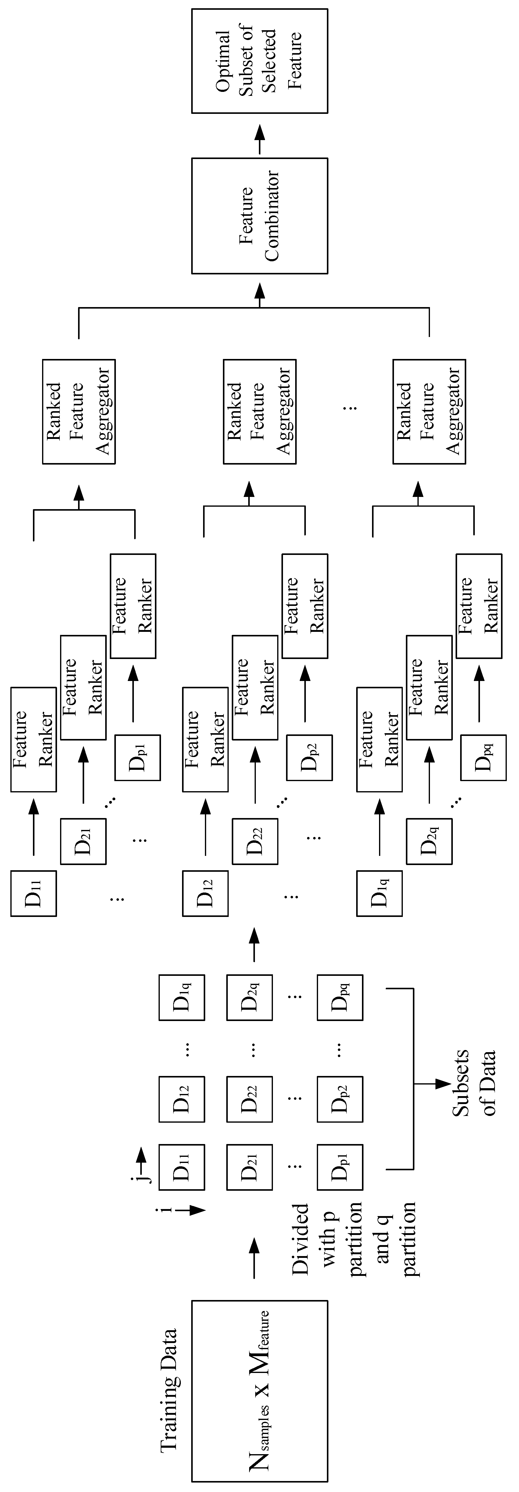
Firstly, the training data were partitioned into several subsets. Then, feature selection was performed on each subset of the data. The results of feature selection and feature ranking were then aggregated to get several new subsets of selected features. Subsets of selected features were then combined to get the most optimal feature subset. Guyon and Elisseeff [1] showed that selecting a subset of features is more useful for excluding redundant features than selecting the most relevant feature. Figure 4 shows a detailed illustration of the proposed framework.

2.3.1. Data Partitioning

Data normalization was carried out before partitioning the data. The purpose of data normalization is to uniform the distribution of values of the data. Equation (1) shows the simplest way of achieving data normalization.

$$norm\_data=\frac{\mathrm{data}-\min (\mathrm{data})}{\max (\mathrm{data})-\min (\mathrm{data})}.$$

(1)

the normalized data were then divided into training data and testing data with a ratio of 7:3. The training data with the N_samples × M_features dimension were then divided into several subsets. Equation (2) shows how the data partition was achieved.

$$tr.dat{a}_{partition}=\frac{1}{p}(N)\times \frac{1}{q}(M),$$

(2)

where p | N and q | M; both p and q are non-zero positive integers = {1, 2, …, N/M}; if p = q, then the equation becomes

$$tr.dat{a}_{partition}=\frac{1}{p}(N\times M)=\frac{1}{q}(N\times M).$$

(3)

2.3.2. Feature Ranker

ReliefF [5] is a Relief [3] filter method. The ReliefF feature selection method is an improvement of Relief that can deal with noisy, multiclass datasets with low bias. This algorithm works by estimating the features according to how well they distinguish neighbor samples. ReliefF is a ranker method; thus, a threshold is needed to obtain the subset of features. The following equation shows how to calculate the weight on Relief:

$$W_i=W_i-diff(x,nearHit)+diff(x,nearMiss),$$

(4)

where W is the weight, x is the feature vector, nearHit is the feature vector closest to x with the same class, and nearMiss is the feature vector closest to x with a different class. Weight W decreases if the difference between feature vectors in the same class is higher than feature vectors in different classes, and vice versa.

The calculation of diff(x, nearHit) and diff(x, nearMiss) using ReliefF is different from that using standard Relief. Whereas standard Relief uses Euclidean distance, ReliefF uses Manhattan distance. Equation (5) shows the calculation formulation using Manhattan distance using ReliefF.

$$diff(x,nearHit|nearMiss)={\displaystyle \sum _{i=1}^n}|x_i-nearHi{t}_i|+|x_i-nearMis{s}_i|.$$

(5)

After the weight W obtained, the next step is to sort W by the most significant value to get feature ranking using the following equation:

$$Relief{F}_{ranking}(p,q)={\displaystyle \sum _{i=1}^p\sum _{j=1}^q}sort(w_{i,j},“ascending”).$$

(6)

2.3.3. Ranked Feature Aggregator

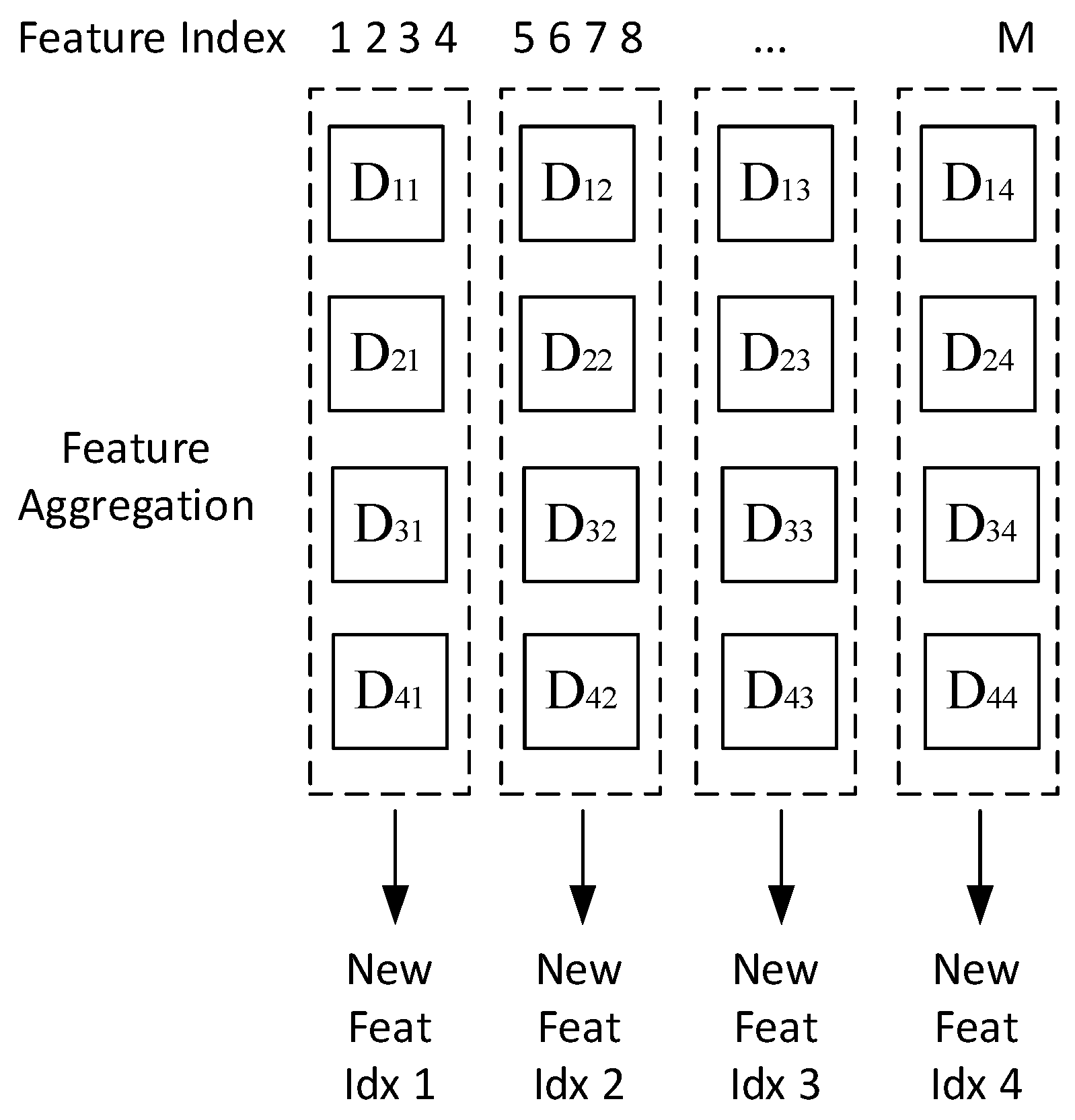
After ranking features in all subsets, the next step is to aggregate each of these features according to the index. Let us assume that the number of partitions in a row and column is the same (p = q). If the number of partitions is four, then there are 16 subsets formed {D₁₁, D₁₂, D₁₃, D₁₄, D₂₁, D₂₂, D₂₃, D₂₄, …, D₄₄}. Aggregation is performed for each subset of the same column {(D₁₁, D₂₁, D₃₁, D₄₁), (D₁₂, D₂₂, D₃₂, D₄₂), …}; this is because the same column has the same feature index and, thus, they can be compared. Figure 5 shows an illustration of feature aggregation.

As illustrated in Figure 5, a group of new features “New.Feat.Idxj” was obtained by finding the mode value of the feature in each subset D in the i row and j column. Equation (7) shows how the feature aggregation works.

$$New.Feat.Id{x}_j={\displaystyle \sum _{j=1}^q\sum _{i=1}^p}mode(D_{ij}).$$

(7)

The threshold k was then applied to these groups. This threshold is a percentage value of how many features reduce. There is a difference between the use of thresholds in ensemble and non-ensemble feature selection. In non-ensemble feature selection, a threshold is applied in all features. In ensemble feature selection, a threshold is applied in the subset of features.

2.3.4. Feature Combinator

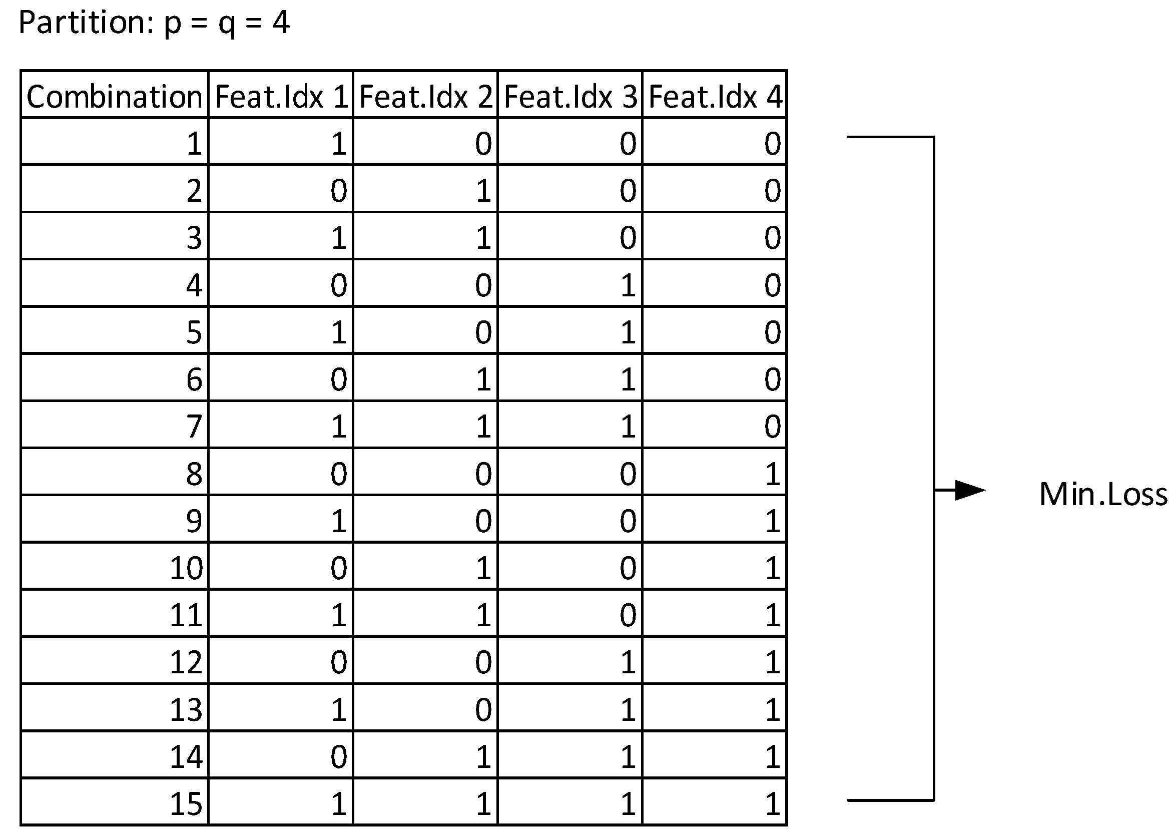
In our previous research [32], a combination was done by combining all features in each subset. Apparently, combining all subsets of features does not produce the best performance. Thus, to solve this problem, we looked for min.loss from all possible combinations of the subsets of features. Figure 6 shows all possible feature combinations if n = 4. Equation (7) shows all possible combination for subsets of features with n subsets.

$$All.Comb={\displaystyle \sum _{k=1}^n}\frac{n!}{k!(n-k)!},$$

(8)

$$Best.FeatSubs=min.Loss(All.Comb),$$

(9)

where n has the same value as p and q. If n = 4, the total possible combination is 15.

2.4. Evaluations

There are several ways to evaluate the performance of ensemble feature selection. The first involves the overall performance of the algorithm. In this evaluation, we can use calculation metrics such as accuracy, precision, recall, specificity, and F1-score.

$$Accuracy(ACC)=\frac{TP+TN}{TP+TN+FP+FN},$$

(10)

$$Precision(PRE)=\frac{TP}{TP+FP},$$

(11)

$$Recall(REC)=\frac{TP}{TP+FN},$$

(12)

$$Specificity(SPE)=\frac{TN}{TN+FP},$$

(13)

$$F1-score(F1)=2(\frac{Precision\times Recall}{Precision+Recall}),$$

(14)

where TP is true positive, TN is true negative, FN is false negative, and FP is false positive.

The second evaluation approach involves the stability of the ensemble feature selection itself. There are three categories for stability measurement, which are stability by index/subset, stability by rank, and stability by weight [38,39]. Stability by rank and weight has a major drawback that does not allow stability calculations on two subsets of features that have different numbers of features. On the contrary, stability by index/subset can deal with different sizes of feature vectors. The mechanism involves the subset of a feature represented as a binary vector, where selected features are represented as 1 and non-selected features are represented as 0. However, stability by rank and weight is more representative when measuring the stability of ranking-based feature selection.

We used these three types of stability to see variations in their stability values. Equation (15) shows a measure of stability by index/subset, i.e., Hamming distance.

$$Hamming(S_i,S_j)={\displaystyle \sum _{k=1}^M}|S_{ik}-S_{ik}|,$$

(15)

$$Normalize\_Hamming(S_i,S_j)=1-\frac{Hamming(S_i,S_j)}{M},$$

(16)

where S_i is subset feature i, and S₂ is subset feature j. M is the total number of features in the dataset. The drawback of this stability measure is that it does not depend on feature rank.

Equation (17) shows a measure of stability by rank, i.e., Spearman’s correlation.

$$Spearman(R_i,R_j)=1-\frac{6\sum d^2}{M(M^2-1)},$$

(17)

where R_i is ranked feature i, and R_j is ranked feature j. The distance between the same feature in R_i and R_j is notated by d. The drawback of this stability measure is that it cannot handle subsets of features from different cardinality, and that two features must at the same size.

Equation (18) shows a measure of stability by weight, i.e., Pearson’s correlation. For Spearman and Pearson correlations, we use the interpolation method to overcome the problem of differences in the number of features.

$$Pearson(W_i,W_j)=\frac{\sum (W_{it}-{\mu }_{w_i})(W_{jt}-{\mu }_{w_j})}{\sqrt{\sum {(W_{it}-{\mu }_{w_i})}^2\sum {(W_{jt}-{\mu }_{w_j})}^2}},$$

(18)

where W_i is weight feature i, and W_j is ranked feature j. ${\mu }_{w_i}$ is the mean of W_i between the same feature in Ri and Rj. The drawback of this stability measure is that two subsets of features must have the same size.

3. Results and Discussion

In this section, we describe some of the results obtained. We evaluated the proposed method based on several criteria. First, the overall performance was judged based on the values of accuracy, recall, specificity, precision, F1-score, and the number of features selected. In this evaluation, we compared the proposed method with previous two-dimensional (2D) ensemble methods and the standard ReliefF. The most important thing from feature selection is knowing which features/subsets of features are relevant. By using a combination method to combine subsets of features and obtain features that produce the smallest loss, we could deduce which subset of features was the most relevant. The next evaluation approach involved measuring the stability of the proposed method. The last evaluation approach involved looking at the effect of the automatic threshold on the proposed method.

3.1. Feature Selection Performance

Table 2. Feature selection performance.

Datasets	Algorithms	ACC	REC	SPE	PRE	F1
MADELON	ReliefF	75.26	73.85	76.67	75.99	0.75
	CFS	48.21	51.79	44.62	48.33	0.50
	mRMR	70.00	73.08	66.92	68.84	0.71
	FCBF	69.87	67.95	71.79	70.67	0.69
COIL20	ReliefF	94.44	100.00	94.15	47.83	0.65
	CFS	93.98	100.00	93.66	45.83	0.63
	mRMR	94.21	100.00	93.90	46.81	0.64
	FCBF	92.59	100.00	92.20	40.74	0.58
USPS	ReliefF	88.45	95.48	87.05	59.60	0.73
	CFS	89.17	96.13	87.78	61.15	0.75
	mRMR	89.60	94.84	88.55	62.38	0.75
	FCBF	86.20	93.98	84.64	55.04	0.69
CTG	ReliefF	98.27	99.40	94.33	98.40	0.99
	CFS	96.86	98.19	92.20	97.79	0.98
	mRMR	86.03	94.15	57.45	88.61	0.91
	FCBF	97.65	98.39	95.04	98.59	0.98
11-TUMORS	ReliefF	67.31	50.00	68.00	5.88	0.11
	CFS	61.54	0.00	64.00	0.00	NaN
	mRMR	76.92	50.00	78.00	8.33	0.14
	FCBF	55.77	0.00	58.00	0.00	NaN

shows the performance evaluation of feature selection. There were four feature selection methods compared, including ReliefF as a baseline, correlation feature selection (CFS), minimum-redundancy maximum-relevancy (mRMR), and fast correlation-based filter (FCBF). We tested them in five datasets representing each field of knowledge. From the comparison results, it was found that ReliefF had the best performance among other methods in three datasets. Therefore, ReliefF was used as a baseline in this paper.

3.2. Overall Performance

Table 3. Performance evaluation.

Datasets	Algorithms	ACC	REC	SPE	PRE	F1	# of Selected Features
MADELON	ReliefF	75.59	75.54	75.64	75.67	0.76	125
	2D ensemble	69.77	69.74	69.79	69.75	0.70	108.5
	Proposed Method	73.15	73.18	73.13	73.15	0.73	58.9
COIL20	ReliefF	93.43	98.61	93.15	43.90	0.61	256
	2D ensemble	95.42	100.00	95.17	52.60	0.69	224.1
	Proposed Method	96.00	99.09	95.83	55.81	0.71	157.1
GISETTE	ReliefF	93.29	92.74	93.84	93.78	0.93	1250
	2D ensemble	93.28	93.05	93.51	93.49	0.93	1091.9
	Proposed Method	93.87	93.86	93.88	93.88	0.94	700.7
USPS	ReliefF	88.64	95.88	87.19	60.06	0.74	64
	2D ensemble	90.12	95.85	88.97	63.56	0.76	57.6
	Proposed Method	90.12	95.85	88.97	63.56	0.76	57.6
YALE	ReliefF	54.69	58.33	54.41	9.25	0.16	256
	2D ensemble	56.33	70.00	55.43	9.38	NaN	222.9
	Proposed Method	60.00	66.67	59.57	9.88	0.17	143
ORL	ReliefF	60.83	50.00	61.11	3.16	0.07	256
	2D ensemble	64.08	43.33	64.62	2.99	0.06	224.4
	Proposed Method	66.00	56.67	66.24	4.04	0.08	127.9
CTG	ReliefF	98.43	99.23	95.59	98.76	0.99	6.00
	2D ensemble	98.60	99.38	95.88	98.84	0.99	4.5
	Proposed Method	98.85	99.52	96.52	99.02	0.99	2.7
11-TUMORS	ReliefF	71.54	80.00	71.20	13.33	0.23	3134
	2D ensemble	74.04	55.00	75.04	9.08	0.22	2715.6
	Proposed Method	77.12	50.00	78.47	9.13	0.22	1320.5
LUNG CANCER	ReliefF	89.50	74.00	90.91	47.30	0.56	3150
	2D ensemble	90.00	82.00	90.73	44.23	0.57	3151.5
	Proposed Method	93.33	94.00	93.27	56.35	0.70	866.8
TOX_171	ReliefF	64.12	68.35	62.60	40.14	0.50	1437
	2D ensemble	52.94	60.27	50.29	30.49	0.40	1360.30
	Proposed Method	65.88	66.15	65.81	41.29	0.50	678.2
PROSTATE_GE	ReliefF	85.67	85.33	86.00	86.78	0.86	1492
	2D ensemble	80.67	80.67	80.67	82.04	0.81	1363.4
	Proposed Method	91.33	90.00	92.67	92.61	0.91	470.4
GLI_85	ReliefF	80.40	64.11	87.03	72.27	0.66	5571
	2D ensemble	80.40	63.75	87.52	70.72	0.65	5572
	Proposed Method	84.80	73.04	89.80	76.07	0.74	1671.6
LYMPHOMA	ReliefF	66.07	83.13	51.24	60.38	0.70	1007
	2D ensemble	64.29	72.20	57.24	60.83	0.66	874.9
	Proposed Method	76.79	89.73	64.95	70.51	0.79	412.1
SMK_CAN_187	ReliefF	57.68	52.22	62.76	57.03	0.54	4999
	2D ensemble	63.21	61.11	65.17	62.44	0.62	5000
	Proposed Method	71.07	68.52	73.45	70.95	0.69	2750

shows the performance evaluation of the proposed method. The proposed method was compared with the previous 2D ensemble methods and the standard ReliefF. We can see that the proposed method outperformed the two comparison methods in all datasets except one, MADELON. When viewed in the MADELON dataset, the proposed method improved the accuracy results from the previous method by 3%, although it was still inferior to the ReliefF standard by a difference of 2%. Exploring further, we found that there were some unsatisfactory results, especially for F1-score. The F1-score for the YALE and ORL datasets was very low, ranging from 0.05 to 0.17. These results were obtained because the recall was too high, but the precision was small. This problem could be overcome using other classification methods.

Another point of performance evaluation was the number of relevant features selected. From these results, the proposed method produced the fewest number of features compared to the other two methods. This result relates to the aggregation and combination method used. As stated earlier, aggregation was done for each subset of features, not the full features in the data. This mechanism is akin to doing multiple thresholds in the ensemble partition. For combinations, the mechanism is to choose a subset of features that have a minimum loss, and those selected have the smallest combination, automatically having the fewest number of features. Overall, the proposed method outperformed the two other methods with a difference of 0.5–14% in terms of accuracy and reduced 50% of features compared other methods.

3.3. Subset of Relevant Features

The primary purpose of feature selection is to determine the features/subset of features that are relevant and not relevant in a dataset. Therefore, in this evaluation, we described which subsets of features were relevant in the tested dataset.

Table 4. Subset of selected features.

Dataset	#1 Run	#2 Run	#3 Run	#4 Run	#5 Run	#6 Run	#7 Run	#8 Run	#9 Run	#10 Run	Intersection
MADELON	10	8	11	15	10	8	14	14	10	13	2 and 4
YALE	12	11	9	10	11	13	15	10	5	15	1 and 4
ORL	5	3	6	3	7	12	7	12	3	12	1 and 3
CTG	13	12	9	11	8	9	9	11	9	9	1 and 4
TOX_171	1	13	7	4	5	8	1	15	13	9	1 and 3
PROSTATE_GE	8	8	8	5	2	1	7	8	8	13	1 and 4
GLI_85	1	8	6	1	5	2	1	1	2	1	1 and 2
LYMPHOMA	1	7	8	9	11	6	4	8	7	12	1 and 4
SMK_CAN_187	2	14	9	3	3	7	2	12	15	10	2 and 4

shows the results of the most relevant subsets of features (with a minimum loss) for 10 trials of each dataset.

For the MADELON dataset, the #1 run resulted in minimum loss with the 10th combination; referring to Figure 6, this means that the feature subsets contained in the combination were the second and fourth feature subsets. Then, for 10 trials, we found that the highest intersection involved the second and fourth subset features. For the CTG dataset, most intersections were in the subsets of the first and fourth features. The features listed in the first subset were the first features, and those listed in the fourth subset were the 20th and 22nd features. If observed further, the first feature in the CTG dataset was the Fetal Heart Rate (FHR) baseline, the 20th feature was the variance histogram, and the 22nd feature was the FHR pattern. These results indicate that, by using this combination, we could also determine which subsets of features were most relevant in a dataset.

3.4. Stability Measurement

Each stability measurement has its advantages and disadvantages. This evaluation was carried out to measure the stability of the proposed method. This also elaborated on the capabilities of the considered stability measures. By using Hamming distance, we converted the feature ranking into a binary representative.

Table 5. Feature generation of the proposed method on the CTG dataset.

Iteration	Selected Feature	Feature Representative
1	[1 13 22 20]	[1000000000001000000101]
2	[13 22 18]	[0000000000001000010001]
3	[1 22 20]	[1000000000000000000101]
4	[1 7 22]	[1000001000000000000001]
5	[22]	[0000000000000000000001]
6	[1 22 20]	[1000000000000000000101]
7	[1 22]	[1000000000000000000001]
8	[1 7 22 20]	[1000001000000000000101]
9	[3 22]	[0010000000000000000001]
10	[3 22]	[0010000000000000000001]

shows the feature generated on the CTG dataset from the proposed method in 10 iterations.

Table 6. Stability measurement comparison on the CTG dataset.

			Hamming	Spearman	Pearson
A	[1 13 22 20]	[1000000000001000000101]	0.991	0.800	0.908
B	[13 22 18]	[0000000000001000010001]
A1	[1 7 22 20]	[1000001000000000000101]	0.991	0.800	0.915
B1	[3 22]	[0010000000000000000001]
A2	[1 22 20]	[1000000000000000000101]	0.991	1.000	0.931
B2	[13 22 18]	[0000000000001000010001]
A1	[3 22]	[0010000000000000000001]	0.995	1.000	1.000
B2	[1 22]	[1000000000000000000001]

shows the performance comparison of stability measurement on the CTG dataset. From this result, it can be said that the measurement of stability using Hamming distance had an outstanding value. This is because the difference was based only on binary values. Spearman stability showed that, if the features had the same amounts and similarities, the result was 1. Stability using Pearson’s correlation in this experiment had more variation values. Overall, the proposed method had excellent stability, ranging from 0.8–1.

3.5. Applying Automatic Threshold

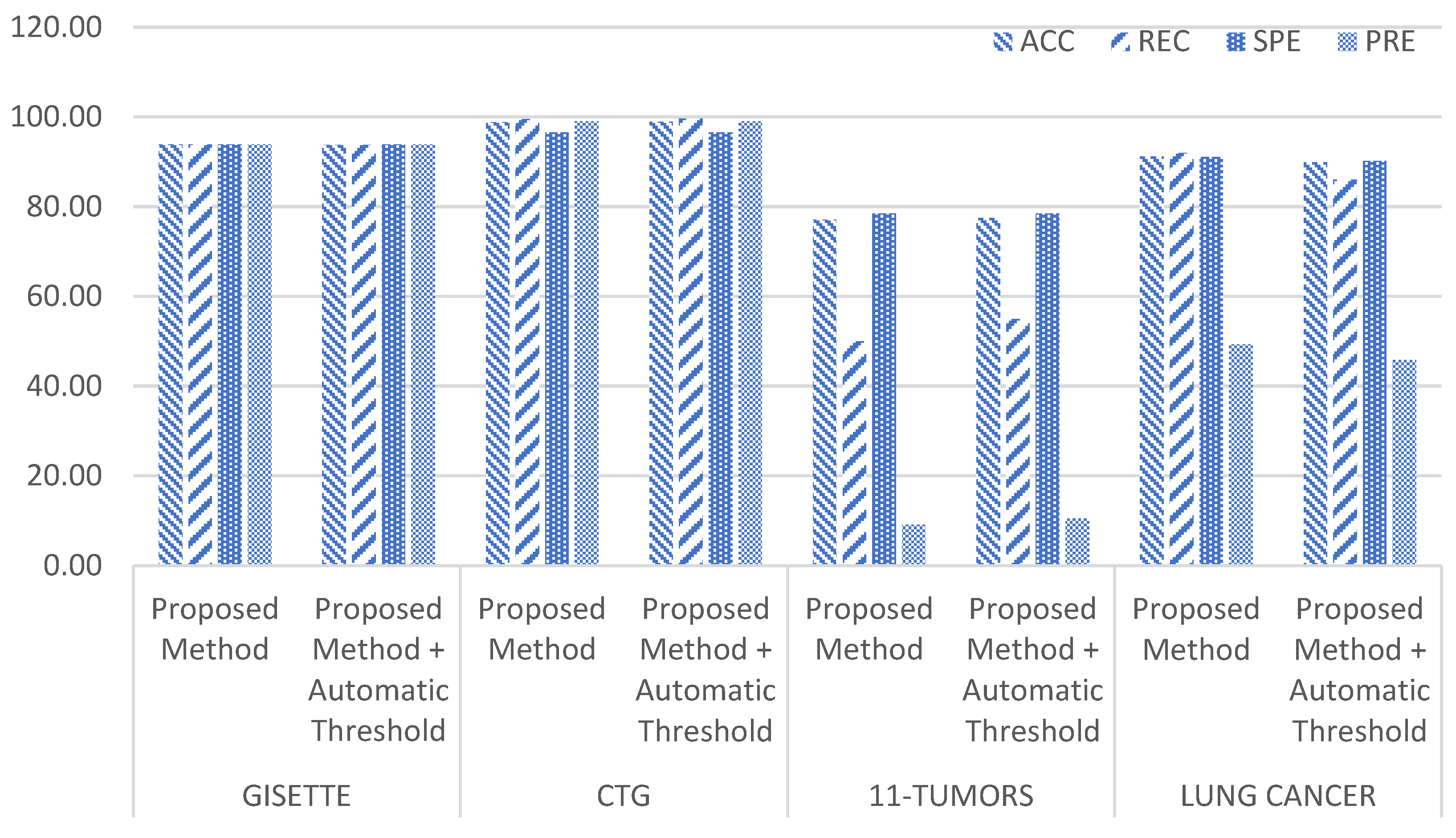
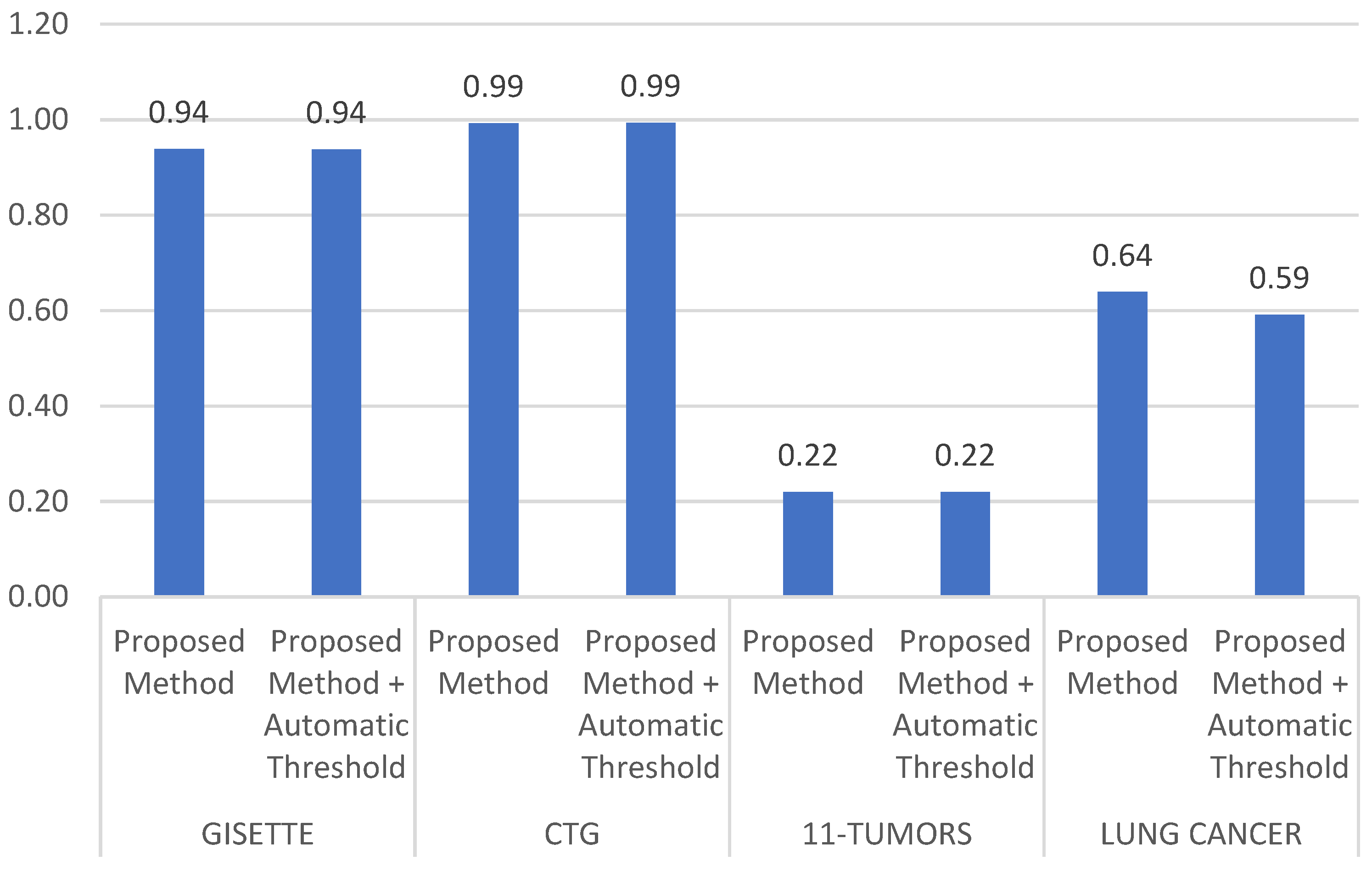
We also applied an automatic threshold to the proposed method. The automatic threshold used was the mean of the ranking weight. Figure 7 and Figure 8 show the results of a comparison between the proposed method without an automatic threshold and that using the automatic threshold. The result was not significant; in some cases, the results with an automatic threshold surpassed those without an automatic threshold, and vice versa.

4. Conclusions and Future Works

In this paper, we presented an improvement of the homogeneous distribution ensemble feature selection with a two-dimensional partition method. The improvement was in the feature aggregation and feature combination. From the results obtained, the proposed method optimally always produced the best performance in terms of both accuracy and feature reduction. The accuracy comparison between the proposed method and other methods was 0.5–14%, and it reduced more features than other methods by 50%. The stability of the proposed method was also excellent, with an average of 0.95. Finally, using the proposed method, we could determine which combination of subsets of features produced a better result.

Although the proposed method gave excellent performance, there were still some limitations that need to be addressed. The future work of this research will focus on how to implement an effective and efficient automatic threshold using this method. we will also study how to improve F1-scores by implementing other classification methods such as deep learning.

References

- Guyon, I.; Elisseeff, A. An Introduction to Variable and Feature Selection. J. Mach. Learn. Res. 2003, 3, 1157–1182. [Google Scholar]
- Durgabai, R.P.L. Feature Selection using ReliefF Algorithm. Int. J. Adv. Res. Comput. Commun. Eng. 2014, 3, 8215–8218. [Google Scholar] [CrossRef]
- Kira, K.; Rendell, L.A. Feature selection problem: Traditional methods and a new algorithm. In Proceedings of the Tenth National Conference on Artificial Intelligence, San Jose, CA, USA, 12–16 July 1992. [Google Scholar]
- Kononenko, I. Estimating attributes: Analysis and extensions of RELIEF. In Proceedings of the Machine Learning: ECML-94; Bergadano, F., De Raedt, L., Eds.; Springer: Berlin/Heidelberg, Germany, 1994; pp. 171–182. [Google Scholar]
- Kononenko, I.; Šimec, E.; Robnik-Šikonja, M. Overcoming the Myopia of Inductive Learning Algorithms with RELIEFF. Appl. Intell. 1997, 7, 39–55. [Google Scholar] [CrossRef]
- Urbanowicz, R.J.; Meeker, M.; La Cava, W.; Olson, R.S.; Moore, J.H. Relief-based feature selection: Introduction and review. J. Biomed. Inform. 2018, 85, 189–203. [Google Scholar] [CrossRef]
- Hall, M. Correlation-Based Feature Selection for Machine Learning. Master’s Thesis, University of Waikato Hamilton, Hamilton, New Zealand, 1999. [Google Scholar]
- Chormunge, S.; Jena, S. Correlation based feature selection with clustering for high dimensional data. J. Electr. Syst. Inf. Technol. 2018, 5, 542–549. [Google Scholar] [CrossRef]
- Kohavi, R.H.; John, G. Wrappers for feature subset selection. Artif. Intell. 1997, 97, 273–324. [Google Scholar] [CrossRef] [Green Version]
- Foithong, S.; Pinngern, O.; Attachoo, B. Feature subset selection wrapper based on mutual information and rough sets. Expert Syst. Appl. 2012, 39, 574–584. [Google Scholar] [CrossRef]
- Lee, S.J.; Xu, Z.; Li, T.; Yang, Y. A novel bagging C4.5 algorithm based on wrapper feature selection for supporting wise clinical decision making. J. Biomed. Inform. 2018, 78, 144–155. [Google Scholar] [CrossRef]
- Wang, A.; An, N.; Chen, G.; Li, L.; Alterovitz, G. Accelerating wrapper-based feature selection with K-nearest-neighbor. Knowl.-Based Syst. 2015, 83, 81–91. [Google Scholar] [CrossRef]
- Chen, Y.; Wang, Z.B. Feature selection based convolutional neural network pruning and its application in calibration modeling for NIR spectroscopy. Chemom. Intell. Lab. Syst. 2019, 191, 103–108. [Google Scholar] [CrossRef]
- Zhang, X.; Wu, G.; Dong, Z.; Crawford, C. Embedded feature-selection support vector machine for driving pattern recognition. J. Frankl. Inst. 2015, 352, 669–685. [Google Scholar] [CrossRef]
- Rajeswari, K.; Vaithiyanathan, V.; Neelakantan, T.R. Feature Selection in Ischemic Heart Disease identification using feed forward neural networks. Procedia Eng. 2012, 41, 1818–1823. [Google Scholar] [CrossRef] [Green Version]
- Ghaemi, M.; Feizi-Derakhshi, M.-R. Feature selection using Forest Optimization Algorithm. Pattern Recognit. 2016, 60, 121–129. [Google Scholar] [CrossRef]
- Das, A.K.; Das, S.; Ghosh, A. Ensemble feature selection using bi-objective genetic algorithm. Knowl.-Based Syst. 2017, 123, 116–127. [Google Scholar] [CrossRef]
- Singh, S.; Singh, A.K. Web-Spam Features Selection Using CFS-PSO. Procedia Comput. Sci. 2018, 125, 568–575. [Google Scholar] [CrossRef]
- Kar, S.; Sharma, K.D.; Maitra, M. Gene selection from microarray gene expression data for classification of cancer subgroups employing PSO and adaptive K-nearest neighborhood technique. Expert Syst. Appl. 2015, 42, 612–627. [Google Scholar] [CrossRef]
- Vafaee Sharbaf, F.; Mosafer, S.; Moattar, M.H. A hybrid gene selection approach for microarray data classification using cellular learning automata and ant colony optimization. Genomics 2016, 107, 231–238. [Google Scholar] [CrossRef]
- Ebrahimpour, M.K.; Eftekhari, M. Ensemble of feature selection methods: A hesitant fuzzy sets approach. Appl. Soft Comput. J. 2017, 50, 300–312. [Google Scholar] [CrossRef]
- Sheeja, T.K.; Kuriakose, A.S. A novel feature selection method using fuzzy rough sets. Comput. Ind. 2018, 97, 111–121. [Google Scholar] [CrossRef]
- Wang, L.; Meng, J.; Huang, R.; Zhu, H.; Peng, K. Incremental feature weighting for fuzzy feature selection. Fuzzy Sets Syst. 2019, 368, 1–19. [Google Scholar] [CrossRef]
- Chen, J.; Mi, J.; Lin, Y. A graph approach for fuzzy-rough feature selection. Fuzzy Sets Syst. 2019, 1. [Google Scholar] [CrossRef]
- Liu, Z.; Zhao, X.; Li, L.; Wang, X.; Wang, D. A novel multi-attribute decision making method based on the double hierarchy hesitant fuzzy linguistic generalized power aggregation operator. Information 2019, 10, 339. [Google Scholar] [CrossRef] [Green Version]
- Xia, J.; Liao, W.; Chanussot, J.; Du, P.; Song, G.; Philips, W. Improving Random Forest With Ensemble of Features and Semisupervised Feature Extraction. IEEE Geosci. Remote Sens. Lett. 2015, 12, 1471–1475. [Google Scholar]
- Seijo-Pardo, B.; Porto-Díaz, I.; Bolón-Canedo, V.; Alonso-Betanzos, A. Ensemble feature selection: Homogeneous and heterogeneous approaches. Knowl.-Based Syst. 2017, 118, 124–139. [Google Scholar] [CrossRef]
- Bolón-Canedo, V.; Alonso-Betanzos, A. Ensembles for feature selection: A review and future trends. Inf. Fusion 2019, 52, 1–12. [Google Scholar] [CrossRef]
- Seijo-Pardo, B.; Bolón-Canedo, V.; Alonso-Betanzos, A. On developing an automatic threshold applied to feature selection ensembles. Inf. Fusion 2019, 45, 227–245. [Google Scholar] [CrossRef]
- Drotár, P.; Gazda, M.; Vokorokos, L. Ensemble feature selection using election methods and ranker clustering. Inf. Sci. 2019, 480, 365–380. [Google Scholar] [CrossRef]
- Chiew, K.L.; Tan, C.L.; Wong, K.S.; Yong, K.S.C.; Tiong, W.K. A new hybrid ensemble feature selection framework for machine learning-based phishing detection system. Inf. Sci. 2019, 484, 153–166. [Google Scholar] [CrossRef]
- Alhamidi, M.R.; Arsa, D.M.S.; Rachmadi, M.F.; Jatmiko, W. 2-Dimensional homogeneous distributed ensemble feature selection. In Proceedings of the 2018 International Conference on Advanced Computer Science and Information Systems, ICACSIS 2018, Yogyakarta, Indonesia, 27–28 October 2018. [Google Scholar]
- Dowlatshahi, M.B.; Derhami, V.; Nezamabadi-Pour, H. Ensemble of filter-based rankers to guide an epsilon-greedy swarm optimizer for high-dimensional feature subset selection. Information 2017, 8, 152. [Google Scholar] [CrossRef] [Green Version]
- Guyon, I. NIPS 2003 Workshop on Feature Extraction and Feature Selection Challenge. Available online: http://clopinet.com/isabelle/Projects/NIPS2003/#links (accessed on 17 July 2018).
- Feature Selection Dataset. Available online: http://featureselection.asu.edu/datasets.php (accessed on 2 April 2018).
- Dheeru, D.; Karra Taniskidou, E. Machine Learning Repository. Available online: http://archive.ics.uci.edu/ml (accessed on 2 April 2018).
- Gene Expression Model Selector. Available online: http://gems-system.org (accessed on 10 May 2018).
- Mohana Chelvan, P.; Perumal, K. A Survey on Feature Selection Stability Measures. Int. J. Comput. Inf. Technol. 2016, 5, 98–103. [Google Scholar]
- Khaire, U.M.; Dhanalakshmi, R. Stability of feature selection algorithm: A review. J. King Saud Univ. Comput. Inf. Sci. 2019, in press. [Google Scholar] [CrossRef]
Figure 1.
Sample images in USPS dataset. (http://www.cad.zju.edu.cn/home/dengcai/Data/USPS/images.html).
Figure 2.
Sample images in YALE dataset (http://www.cad.zju.edu.cn/home/dengcai/Data/Yale/images.html).
Figure 3.
Sample images in ORL dataset (http://www.cad.zju.edu.cn/home/dengcai/Data/ORL/images.html).
Figure 4.
2-dimensional distribution ensemble feature selection framework.
Figure 5.
Illustration of feature aggregation in ensemble feature selection.
Figure 6.
All possible feature combinations in ensemble feature selection with p = q = 4.
Figure 7.
Performance (accuracy, recall, specificity, precision) comparison of the proposed method without automatic threshold with the proposed method + automatic threshold.
Figure 8.
F1-Score comparison of the proposed method without automatic threshold with proposed method + automatic threshold.