A GARCH Model with Artificial Neural Networks


Department of Information Systems, Business Statistics and Operations Management, The Hong Kong University of Science and Technology, Clear Water Bay, Hong Kong, China
*
Author to whom correspondence should be addressed.
Information 2020, 11(10), 489; https://0-doi-org.brum.beds.ac.uk/10.3390/info11100489
Submission received: 3 October 2020
/
Revised: 16 October 2020
/
Accepted: 17 October 2020
/
Published: 20 October 2020
Abstract
:In this paper, we incorporate a GARCH model into an artificial neural network (ANN) for financial volatility modeling and estimate the parameters in Tensorflow. Our goal was to better predict stock volatility. We evaluate the performance of the models using the mean absolute errors of powers of the out-of-sample returns between 2 March 2018 and 28 February 2020. Our results show that our modeling procedure with an ANN can outperform the standard GARCH(1,1) model with standardized Student’s t distribution. Our variable importance analysis shows that Net Debt/EBITA is among the six most important predictor variables in all of the neural network models we have examined. The main contribution of this paper is that we propose a Long Short-Term Memory (LSTM) model with a GARCH framework because LSTM can systematically take into consideration potential nonlinearity in volatility structure at different time points. One of the advantages of our research is that the proposed models are easy to implement because our proposed models can be run in Tensorflow, a Python package that enables fast and automatic optimization. Another advantage is that the proposed models enable variable importance analysis.
1. Introduction
GARCH models are popular in finance and economic literature. Bollerslev [1] introduced a GARCH(1,1) model in which the residual term follows a standardized Student’s t distribution. Nikolaev et al. [2] suggested that the GARCH model takes into account the dynamics of time-dependent variance and therefore incorporated a GARCH model into non-linear neural networks. So and Yu [3] compared multiple GARCH models on their performance in value at risk estimation. So and Wong [4] developed expected shortfall and median shortfall estimation under GARCH models. Chen and So [5] extended the GARCH model to have threshold nonlinearity. Chen et al. [6] studied Markov switching GARCH models for volatility forecasting. So and Xu [7] used GARCH models to capture more intraday information. Efimova and Serletis [8] modeled oil, natural gas, and electricity markets using a multivariate GARCH model because it allows for rich dynamics in the variance–covariance structure. Their finding is higher precision in key estimates achieved by using a less computationally demanding model. Kristjanpoller and Minutolo [9] extended their model by applying an artificial neural network (ANN) to the GARCH model. Zhipeng and Shenghong [10] extended the BEKK–GARCH model by applying the Markov regime switching method that incorporates state transformation. Escobar-Anel et al. [11] introduced a class of GARCH models. The daily return at time t can be modeled as follows:
where is a single period return. introduces flexibility so that non-Normal models can be generated. The variable measures the impact of market risk from and r is a risk-free rate. is a non-negative function as that the variances in the model are non-negative. The class of GARCH models can incorporate important empirical characteristics of financial asset returns and derivatives, such as jumps, and have a recursive closed form for a conditional moment generating function. They noted that the class GARCH model can accommodate dynamic volatility, enabling efficient option pricing and an assessment of risks. Mercuri [12] extended the GARCH model for option pricing by defining a tempered stable distribution, which enables lighter tail of real financial data.
A standard GARCH model, however, may not capture the information and predict the distributions of returns effectively because the relationship between the current variance and the variance on the previous day may not be linear. Nikolaev et al. [13] found that for the dataset consisting of DEM/GBP currency exchange rates between 3 January 1984 to 31 December 1991, an RNN–GARCH model’s performance can improve statistical characteristics, where RNN is a recurrence neural network. Nikolaev et al. [2] suggested that their recurrent network has better results and is more accurate than linear models. Kristjanpoller and Minutolo [9] applied an artificial neural network to the GARCH model because with this approach a neural network architecture can help to detect nonlinear patterns. They noted that by incorporating nonlinearity into the GARCH model, an ANN–GARCH model shows a 25% reduction in mean absolute percentage errors for gold spot price and gold future price data collected from Bloomberg. Kristjanpoller and Minutolo [14] showed that an ANN–GARCH model improves the prediction of future oil prices. Liu et al. [15] used an asymmetric GARCH process for deposit insurance pricing in which the conditional covariance depends on the conditional variance, the square root of the conditional variance and the perturbation from the previous period. Kim and Won [16] proposed a hybrid model integrating Long Short-Term Memory (LSTM) with multiple GARCH-type models to incorporate nonlinearities in the model. Ardia et al. [17] defined different tail and asymmetry parameters for different states in a GARCH model in order to incorporate regime changes in their volatility dynamics. Cheikh et al. [18] applied a logistic function in the conditional variance equation of a GARCH model in order to capture the asymmetric behavior of bad news compared to good news.
To summarize, GARCH models are popular in finance and economic literature [1,2,3,5,6,7,8,9,10,11,12]. However, standard GARCH models may not capture the volatility dynamic adequately because the relationship between the current variance and the variance on the previous day may not be linear [2,9,13,14,15,16,17,18]. Kristjanpoller and Minutolo [14] showed that an ANN–GARCH model improves the prediction of future oil prices. Kim and Won [16] proposed a hybrid model integrating LSTM with multiple GARCH-type models to incorporate nonlinearities in the model. These inspired us to develop a hybrid model: LSTM model in the GARCH framework.
There are several notable differences between our proposed models and Kristjanpoller and Minutolo [14]’s model. Firstly, our models systematically incorporate information on the previous days through the use of LSTM, but the approach taken by Kristjanpoller and Minutolo [14] was simply to apply ANN on mostly GARCH forecasts, the square of the oil price return and other financial series to output volatility forecast. Secondly, we use the characteristics of the stock index as inputs. Their first models are built by GARCH forecast and the square of the oil price returns. When their initial model is stable, they include four financial series of data. The list of input variables in their model then changes with time. Consequently, their model building process requires much more time and computation power. Thirdly, the objective functions are deterministic while our objective function takes into account the probabilistic nature of returns. Their objective functions are heteroscedasticity adjusted mean squared error and heteroscedasticity adjusted mean squared error but our objective function is the negative loglikelihood function.
There are obvious differences between our proposed models and Kim and Won [16]’s model. Firstly, their LSTM model inputs include the parameters of GARCH, EGARCH, and EWMA at different times in order to measure the trend factors at different times, indicating that they carried out multiple optimizations for calculation of inputs. This requires more time for training and may accumulate errors in inputs due to a substantial number of objective functions for optimizations. Secondly, their model is more complex than our proposed models, meaning that their model is more prone to overfitting. Thirdly, the objective functions are deterministic while our objective function takes into account the probabilistic nature of returns. Their objective functions are mean absolute error (MAE), mean squared error, heteroscedasticity adjusted MSE and heteroscedasticity adjusted MAE but our objective function is the negative loglikelihood function.
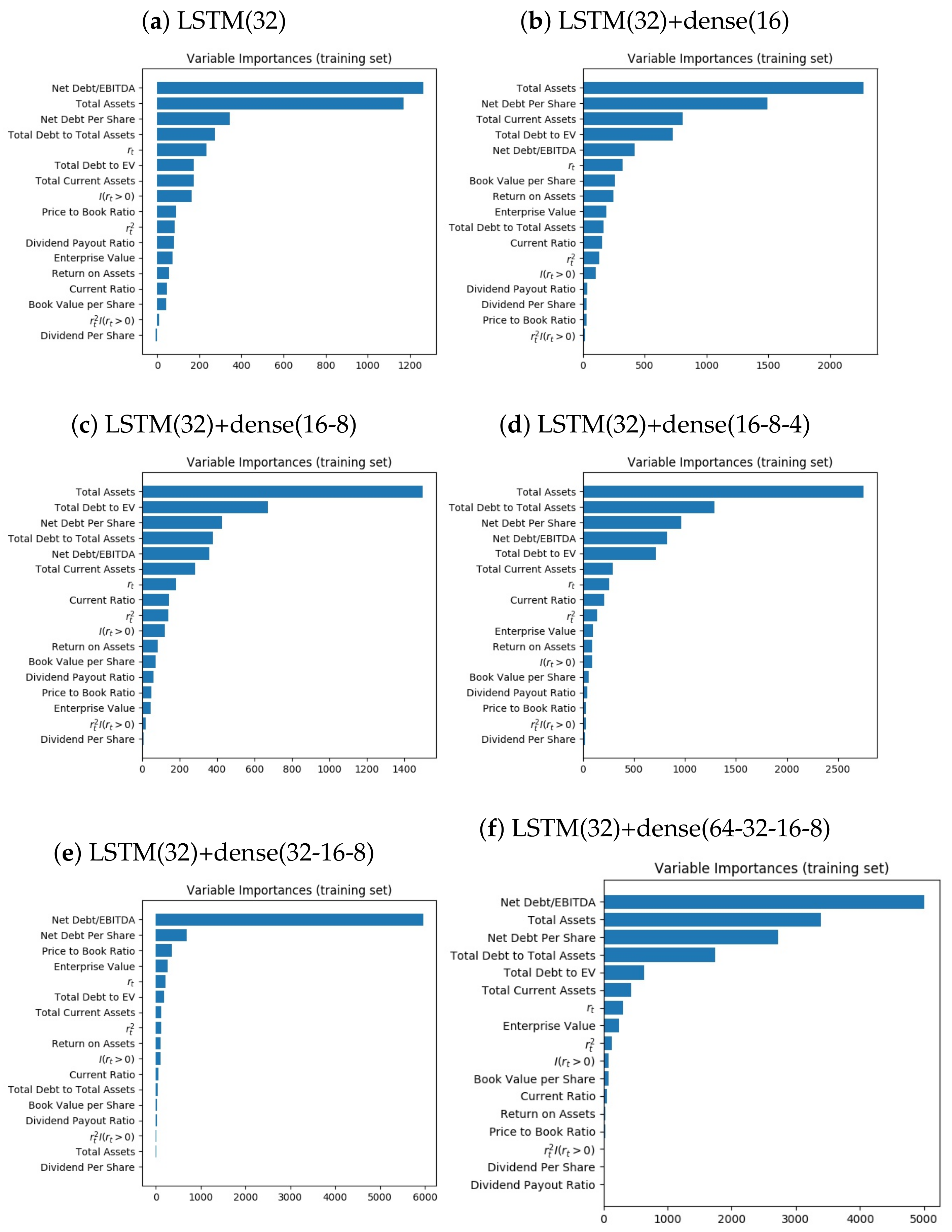
The main contribution of this paper is that it proposes an LSTM model with a GARCH framework. LSTM can systematically take into consideration the potential nonlinearity in a volatility structure at different time points. Therefore, our models are more robust and comprehensive in predicting the volatility of returns. To examine the accuracy of our models, we need to visualize the recurrent network model performances and evaluate metrics of model performances. In order to visualize the recurrent network model performances, we compare the actual returns with the predicted standard deviations and compare the actual squared returns with the predicted variances. In general, the predicted standard deviations increase when the returns fluctuates rapidly. For some of the models, actual and the predicted variance are very close. In addition, to evaluate metrics in the recurrent network models, we calculate the mean absolute errors of absolute returns for the recurrent network models, and compare them with those for the GARCH(1,1) model with standardized Student’s t distribution. The results show that two of the recurrent network models outperform the GARCH(1,1) model with standardized Student’s t distribution. As a result that the models are complex and our aim was to understand the models better, we calculate the variable importance of each of the variables in the data set. The idea of variable importance in this paper is the difference in loglikelihood after removing the variable of interest. Our result shows that Net Debt/EBITA is important in all of the recurrent network models we have examined.
There are two main advantages of the proposed models. The first advantage is that they are easier to implement because the program runs are carried out in Tensorflow. As mentioned in Heaton et al. [19] and Chen et al. [20], it is convenient to set up ANN architectures in Tensorflow. The computational efficiency, which is demonstrated in our numerical experiments, is also an attractive feature of Tensorflow. In Nikolaev et al. [13] and Kristjanpoller and Minutolo [9], it was necessary to write down and compute the derivatives. In Tensorflow, with a standard layer like LSTM, the optimization is automatic and fast after defining the objective function, network structure and commonly used optimization algorithm. The second advantage is that the proposed models enable variable importance analysis. Nikolaev et al. [13], Nikolaev et al. [2], Kristjanpoller and Minutolo [9], and Kristjanpoller and Minutolo [14] did not provide variable importance analysis and therefore did not allow for a thorough understanding by readers of what variables are important in their models. Our paper provides a metric for accessing variable importance to demonstrate which variables are important.
2. GARCH–ANN Construction
2.1. Network Architecture
To forecast variance, the methodology in this study follows a hybrid model: LSTM model and GARCH framework. The model first defines that the return follows a standardized Student’s t distribution with conditional variance . The conditional variance is then modeled by LSTM. The objective function for parameter estimation is the negative loglikelihood.
The GARCH model is commonly used for return modeling because it takes into account the dynamic nature of the conditional variance of the return. The GARCH(1,1) model can be expressed as
The stationary condition of the GARCH(1,1) model is . In Formulas (1) and (2), the return at time t, , follows a normal distribution with mean zero and variance , given the information up to time . The variance at time t is the linear combination of the conditional variance and the squared return at time .
In the GARCH(1,1) model, the current conditional variance is a linear function of conditional variance and the squared return on the previous day. However, this assumption may not hold because the relationship may not be linear. Nikolaev et al. [13] showed that dynamic recurrent network yields results with improved statistical performance. Nikolaev et al. [2] showed an improved result after using a nonlinear recurrent network. The target variable return can be modeled as
where is Student’s t distribution with mean 0, variance 1 and degrees of freedom . Assume that is an information vector at time t.
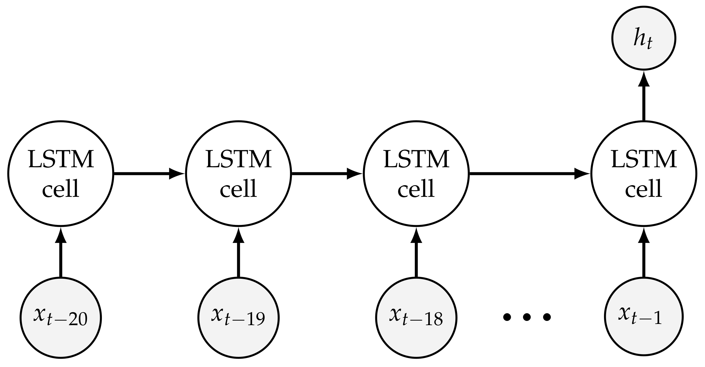
The architecture of is shown in Figure 1. In the model, we use the data on the previous 20 days to predict the conditional variance of the current returns, . If the period used for predicting the variance of the current return is too long, the risk is that the prediction decreases owing to the fact that the earlier data may not reflect the future return structure. If the period used for predicting the variance of the current return is too short, the risk is that the available information may not be utilized to predict the variance of the returns. However, the numbers of days of data used for prediction of the returns can be changed according to users’ preferences.
Assume that input row vector in LSTM cell is . The LSTM cell can be represented by
where is the m-th element of for . The terminology in LSTM models can be found in Hochreiter and Schmidhuber [21] and Gers et al. [22]. Here, , , and are parameters to be estimated in the model; and are activation functions of output gate and input gate respectively, and the default activation functions are sigmoid functions in Tensorflow; is internal state; is an activation function for cells and the default activation function is a hyperbolic tangent function in Tensorflow; is a differentiable function that scales an memory cell from an internal state, and the default function, , is a hyperbolic tangent function in Tensorflow. Equations (3) and (4) compute the output and input gate activation, respectively. In Equation (5), the internal state is calculated by adding squashed and gated input to the previous internal state . Then, in Equation (6), the cell output is calculated by multiplying the output gate activation with internal states squashed by .
LSTM models can help understand the long-distance relationship between volatility and the explanatory variables. He et al. [23] compared an LSTM model with other neural network models when predicting students’ performance in a specific course. They discussed that LSTM can memorize longer sequence and achieve better results for tasks requiring understanding of long-distance relationship.
After running 20 LSTM cells as specified in Figure 1, we use a deep network to output . Assume that is a deep neural network as in Feng et al. [24]. Then, can be represented by
where is a deep learning architecture consisting of dense layers. In the deep learning architecture with function , the number of hidden units and number of layers are as specified in Feng et al. [24]. The activation functions may not be Rectified Linear Unit (RELU) functions because we experimented with different activation functions and found that the model performance depends on the activation functions.
In the neural network, the backpropagation and chain rule are used when computing the gradients of the objective function. The LSTM layer is considered to be the first layer in Tensorflow and, therefore, we can use the default functions without worrying about gradient issues. However, when considering the activation functions in , we prefer the activation functions that do not result in diminishing/exploding gradient issue. To assess this issue, we tried an RELU and identity function. In our experiment, the identity function works better for this network because RELU may introduce a zero gradient in some regions.
To model non-negative volatility, a mapping from neural network output to a non-negative number is required. Dugas et al. [25] introduced a softplus function as sigmoid’s primitive. They discussed that a softmax function is differentiable and has positive derivatives. Senior and Lei [26] explained that the reason for using a softplus function in neural network is that unlike an RELU, a softplus function does not have a zero gradient in regions, which enables easier training. They found that a neural network with a softplus function shows an improved performance and faster convergence. Consequently, we apply a softplus function to the output from LSTM cells in (7).
2.2. Objective Function
We follow the approach by Nikolaev et al. [2] who applied a maximum likelihood approach in their proposed models. Assume that denotes Student’s t density function with a mean , variance , and degree of freedom . The objective function is
where
The default optimization in Tensorflow is to minimize the objective function and therefore the negative loglikelihood objective function is used.
3. Data Processing
The target stock is the S&P 500 Index. After the removal of data entries for holidays, the data consisted of 17 variables with 5032 observations between 29 February 2000 and 28 February 2020 from the Bloomberg Terminal. In the data, the target variable is the daily percentage change in prices. Assume that is the price at time t. According to the definition from Bloomberg, the daily percentage change in prices can be written as
Denote an indicator function as . Variables in the data set and their summary statistics are as follows:
Table 1 shows the S&P 500 Index variables collected from the Bloomberg terminal. In Table 1, Total Assets, Total Current Assets, Net Debt Per Share, Book Value per Share, and Enterprise Value have a substantially higher mean, standard deviation, and range than other variables, indicating that additional effort in normalization or standardization may be needed in order to simplify the training for the neural networks.
Then, we have done the following steps to create training and testing instances for program runs:
- Read the data by pandas in Python.
- Normalize the data set. Assume that x is a vector. We normalize it by
- Create the instances by labeling the data on the previous 20 days as the input and labeling the current return as the target variable.
- Create the training instances (90%) and testing instances (10%).
- Shuffle the training instances.
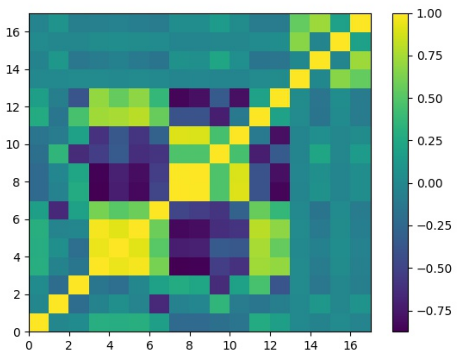
Normalization is crucial for simplifying the tasks in a neural network. Shavit [27] concluded that proper normalization simplifies neural network’s task and improves its ability to control the process. Jayalakshmi and Santhakumaran [28] showed that the performance of diabetes classification is dependent on the normalization method. Yin et al. [29] applied min-max normalization images. As a result that normalization is widely used and can help to simplify the task in the neural network, we opted to apply normalization technique. The interrelationship of the data after normalization can be visualized by the correlation matrix graph shown in Figure 2.
Most of the variables do not have a strong linear relationship, justifying the use of a neural network. After normalization, the instances are created by labeling the data on the previous 20 days as the input and labeling the current return as the target variable. As shown in Figure 1, the inputs and outputs are and for , respectively. The next step is to split the data set into training instances (90%) and testing instances (10%). The instances with the 90% earliest dates are training instances and the rest of instances are testing instances. The target variables for training are in between 28 March, 2000 and 1 March, 2018 while the target variables for testing are in between 2 March, 2018 and 28 February, 2020. The final step is to shuffle the training instances so as to avoid an effect from the ordering of training instances.
4. Training
We have the following specifications for program runs:
- The instances during training are split into batches with size 500 for optimization.
- The optimization algorithm is Adam [30].
- The number of epochs it can tolerate for no improvement is 10.
- The maximum number of epochs is 1000.
During training, the instances are split into batches with a size of 500 for optimization. According to Goodfellow et al. [31], with the minibatch method, the gradient is computed on more than one occasion but fewer than full training examples. They listed a number of reasons for using minibatches in deep neural networks. Minibatches provide a more linear return of accuracy. They also noted that in order to maintain stability due to the high variance in estimation of the gradient, small learning rate needs to be set.
To address the problem of setting appropriate learning rates at each epoch, Adam [30], an adaptive learning rate algorithm, is used in neural network training.The core idea of Adam is that it incorporates a bias correction. In commonly used optimization algorithms such as RMSprop [32], they did not take into account the bias correction even though they accumulated the first order moments and second order moments in the (exponential) average equations. Goodfellow et al. [31] discussed that with early stopping, the algorithm can halt whenever overfitting begins to occur. The number of epochs it can tolerate for no improvement, which is referred as patience in keras, is set to be 10. The maximum number of epochs is 1000, which enables the program to continue running before early stopping. Special care is needed in defining the distribution within the Tensorflow package. Student’s t distribution in Python needs to be standardized by in order to produce the desired results.
5. Empirical Results
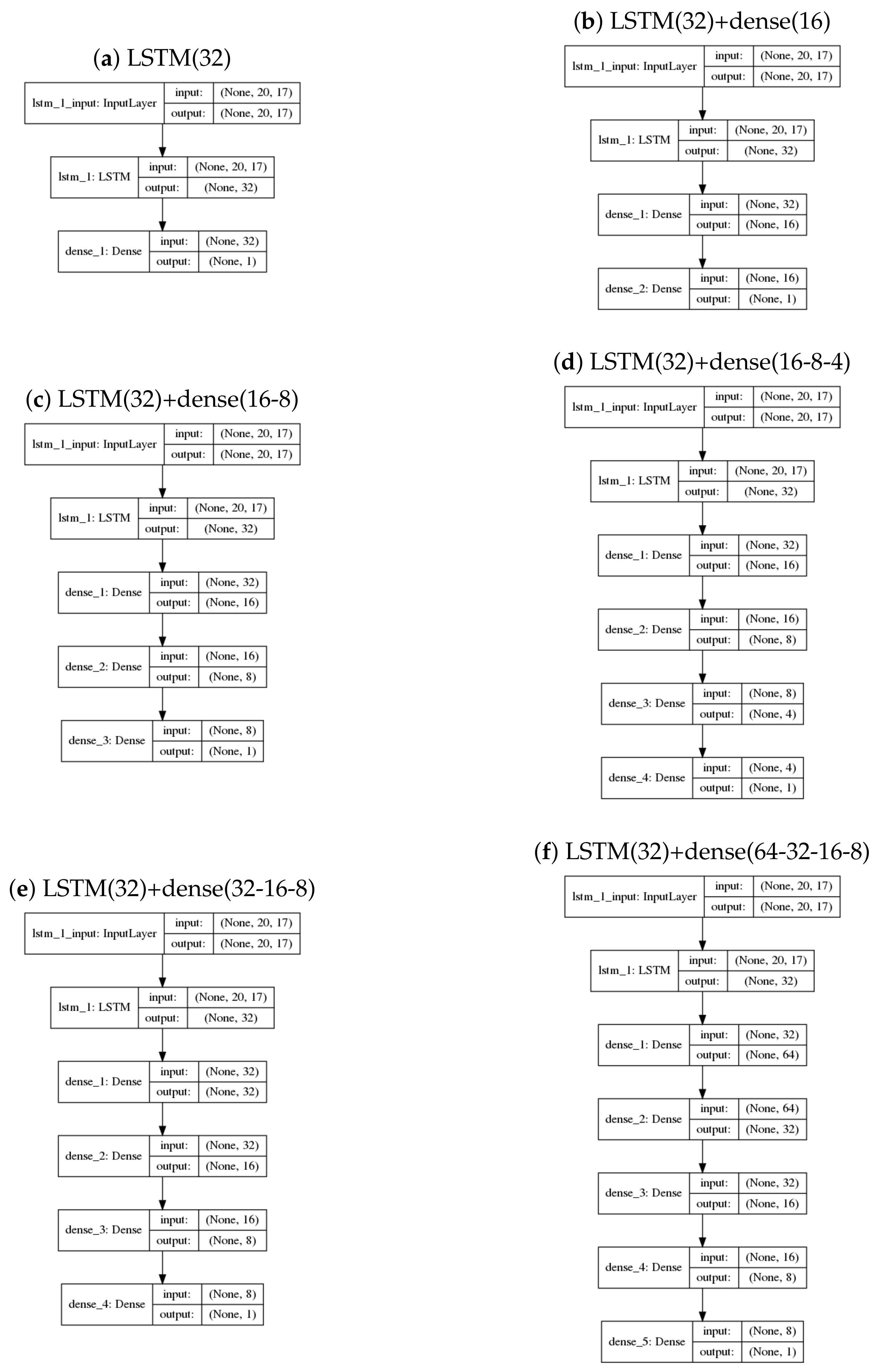
We have produced network diagrams shown in Figure 3 for reference. The shape of each neural network and the names of the layers have been shown in order to give a more extensive view of the architecture. For example, in Figure 3a, the input layer is of dimension 20 × 17 because we use 20 days of data with 17 variables. Architectures such as LSTM(32)+dense(16) and LSTM(32)+dense(16-8) are shown in captions of Figure 4. LSTM(32)+dense(16) means an LSTM layer with 32 units, followed by a dense layer with 16 units. LSTM(32)+dense(16-8) means an LSTM layer with 32 units, followed by two dense layers with 16 units and 8 units, respectively. As LSTM(32)+dense(16-8) contains one more layer than LSTM(32)+dense(16), LSTM(32)+dense(16-8) contains more parameters than LSTM(32)+dense(16). The reason for an LSTM layer with different dense layers in the table is that we would like to see if the difference in dense layers can result in different out-of-the-sample mean absolute error.
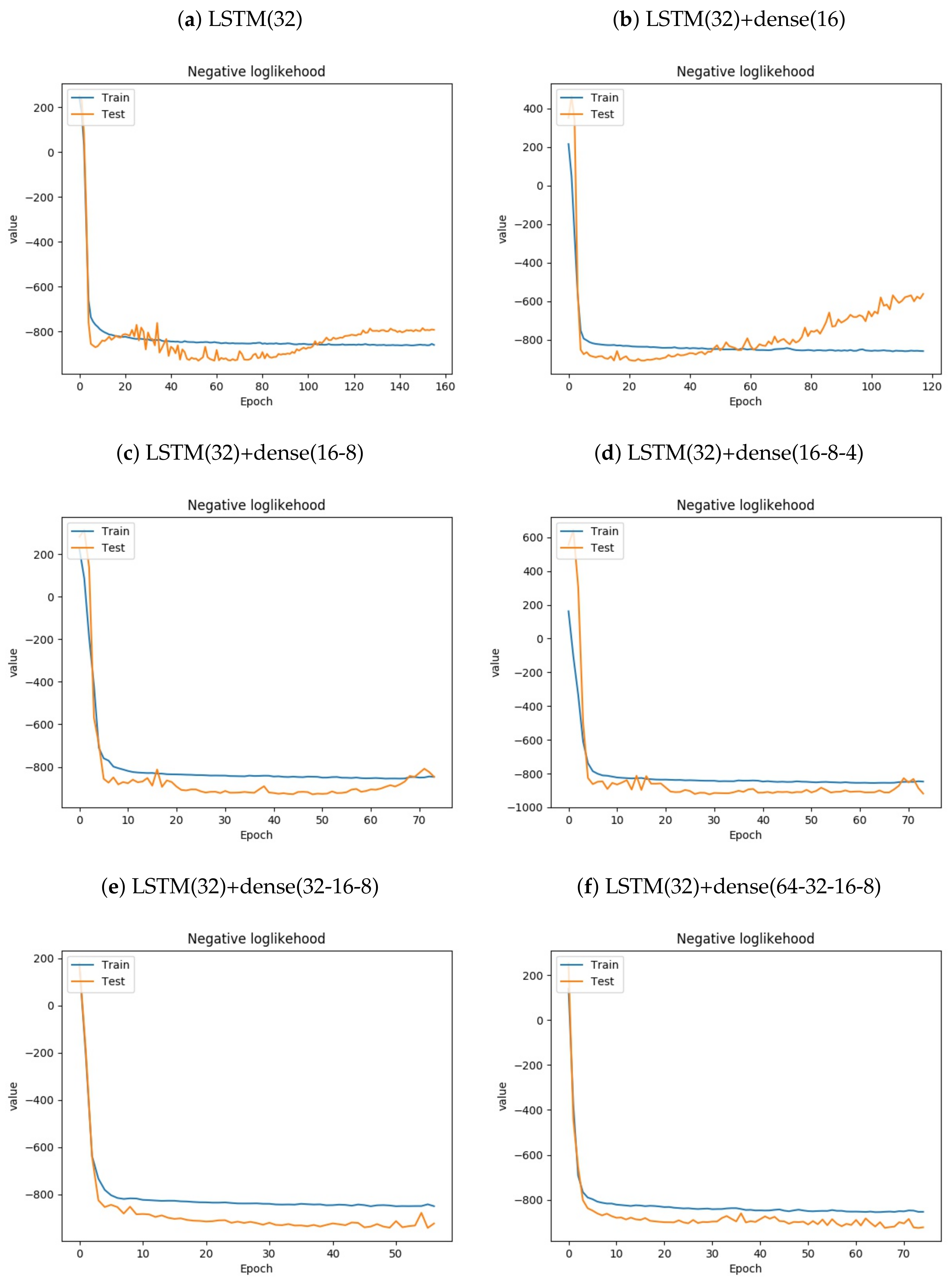
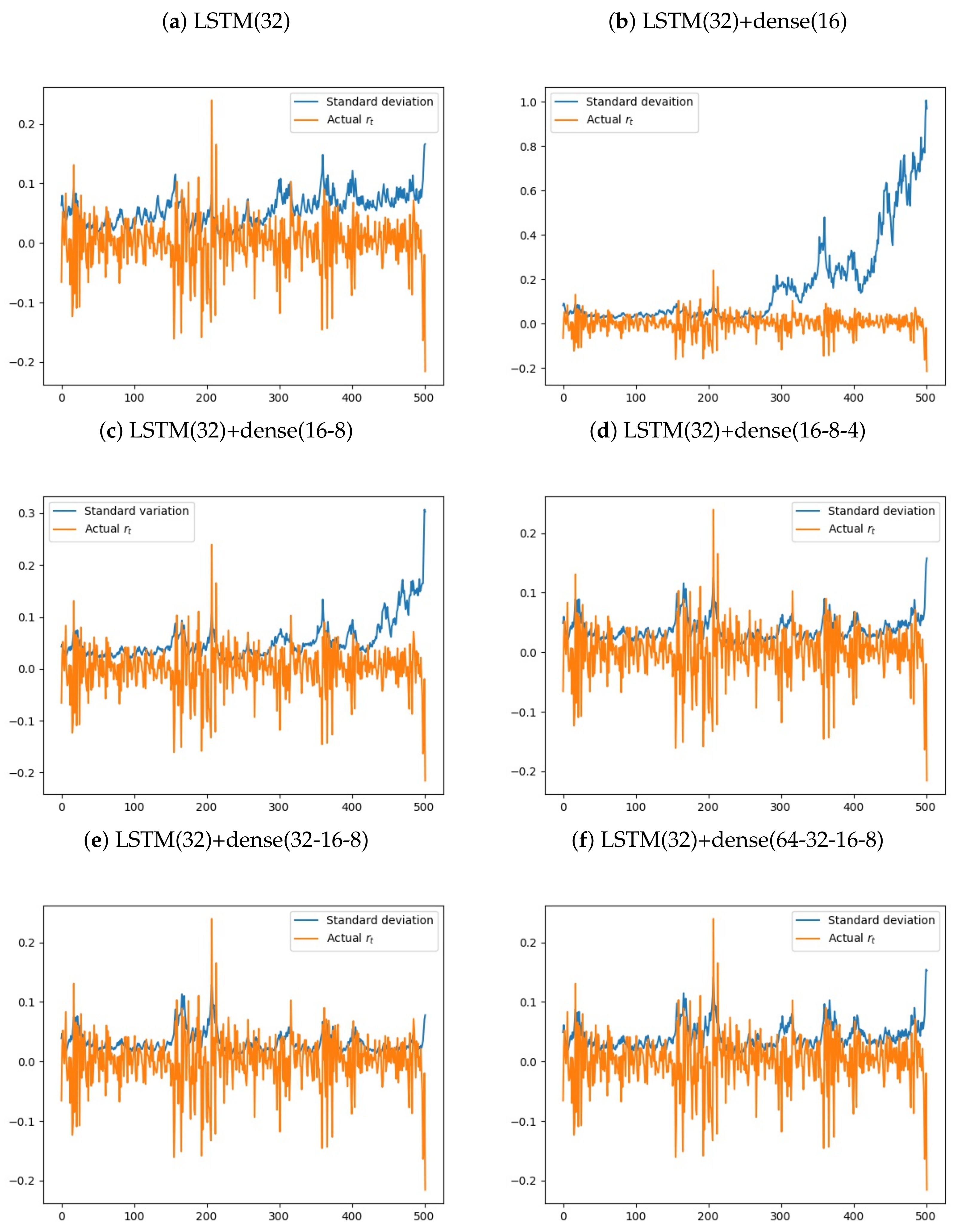
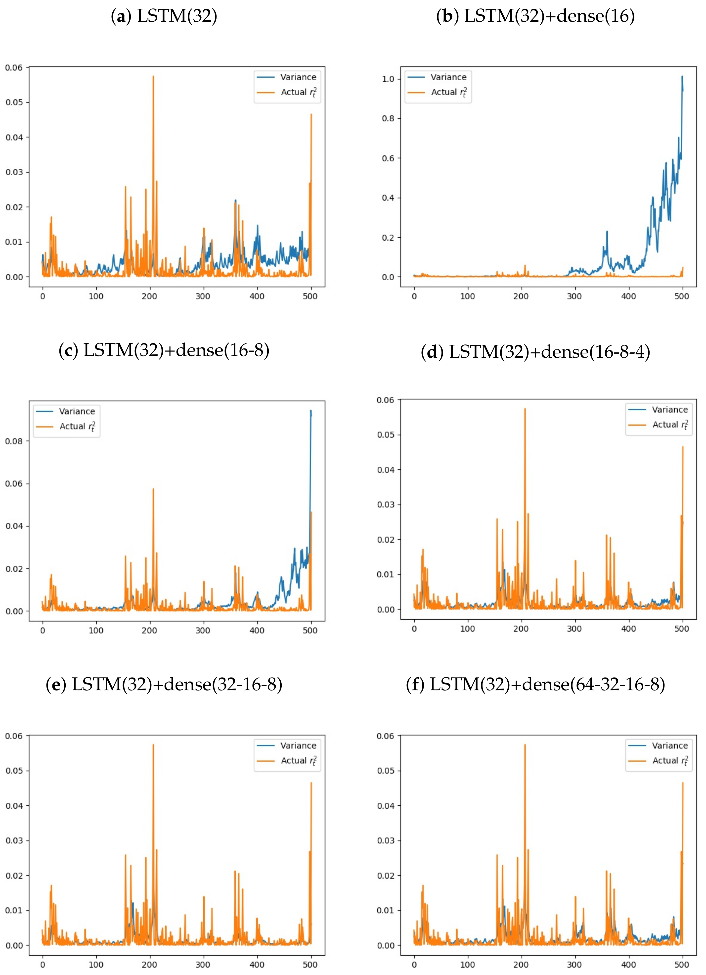
The program runs last for less than two minutes on a CPU-compiled Tensorflow. All of the program runs converge and stop early. To ensure that the program always returns the same results, the random seed in neural networks is set to be zero. After training, we have also drawn training and testing negative loglikelihood over epochs. If the experimental designs are not good, the negative loglikelihoods do not decrease with time. Figure 4 shows the negative loglikelihood over training. As the negative loglikelihood decreases over training for all models except LSTM(32)+dense(64-32-16-8), the overall performance for the training set improved over training. We have also plotted actual and the predicted standard deviation for validation set. If the actual fluctuates rapidly and the predicted standard deviation does not increase, the model does not have high prediction power. Figure 5 shows that except for LSTM(32), the predicted standard deviations increase when the returns fluctuates rapidly. To review the performance of the neural networks, the squared returns and the predicted variances in the testing set are plotted. In Figure 6, except for LSTM(32), actual and the predicted variance are very close.
Forsberg and Ghysels [33] discussed that absolute returns predict volatility better. They showed that absolute returns is immune to jumps. From So and Xu [7] and Winkelbauer [34], we can prove the moments of absolute returns in GARCH model to be
where is a gamma function. So and Xu [7] discussed that the use of can make their evaluation more robust.
Out-of-the-sample mean absolute errors (MAE) in Table 2 are evaluated between 2 March 2018 and 28 February 2020. The model does not change when evaluating the errors. The following steps are taken during MAE:
- Forecast one-step ahead .
- Out-of-the-sample mean absolute error (MAE) is computed by the equation:
To compare the model performances with a standard model, we used an ARCH package [35] to run a GARCH-t(1,1) model which is a standard GARCH(1,1) model, where the residual term at time t () follows standardized Student’s t distribution. The parameters , , and in the Equation (2) are estimated to be 0.2234, 0.1001, and 0.8978, respectively. Their respective p values by t tests are 2.012 × 10, 8.910 × 10, and 0, meaning that the parameters are significant. The package reports that the optimization is robust and the degree of freedom is determined to be 6.7057 by the package. The method used is maximum likelihood estimation, and the final loglikelihood is −13,192.
Compared to the GARCH-t(1,1) model, the two deep learning models performed better as they have smaller out-of-sample errors between 2 March 2018 and 28 February 2020. In terms of MAE for and , LSTM(32)+dense(16-8) and LSTM(32)+dense(32-16-8) outperform GARCH-t(1,1). However, in term of MAE for , the two LSTM models are very close to GARCH-t(1,1). As Forsberg and Ghysels [33] have discussed that realized absolute returns are immune to jumps and are more persistent, it is believed that the MAE for and are more reliable measures, indicating that the two LSTM models outperform GARCH-t(1,1). Out of all the models, in terms of and , LSTM(32)+dense(32-16-8) performs the best. Compared to LSTM(32)+dense(32-16-8), LSTM(32)+dense(64-32-16-8) is more likely to suffer from overfitting because it has one more layer and more parameters.
Variable importance is essential for variable selection. However, there is no universal way to evaluate variable importance in different models. Breiman [36] discussed that for randomly generated input features with weak correlations, the convergence is very slow and the result is poor in the random forest model. He permuted the value of the feature of interest while calculating variable importance. Two Python packages were developed to help researchers calculate the variable importance. Korobov and Lopuhin [37] suggested replacing the feature with random noise when calculating variable importance. Pedregosa Gael Varoquaux Alexandre Gramfort Vincent Michel Bertrand Thirion et al. [38] suggested permuting the input columns of features.
In addition to the two Python packages, caret [39], an R package that has been used for Exam Predictive Analytics by the Society of Actuaries, has taken variable importance into consideration when developing machine learning models. Kuhn [39] defined different kinds of variable importance for different models. For example, in linear regression models, variable importance is defined to be the absolute value of the t-statistic for each model parameter that is used. For the recursive partitioning model, variable importance is defined to be the reduction in the loss function (e.g., mean squared error) attributed to each variable at each split that is tabulated.
To observe which variables are more important, we perform a variable importance analysis. The variable of interest in the input is replaced with zero. Then, the new negative loglikelihood, denoted as , is computed. Assume that is the original loglikelihood. The variable importance for the variable is calculated as follows:
The intuition for this likelihood ratio metric is that the models we are using are probability models and the metric for evaluation is loglikelihood. Note that the variable importance we are using can be negative because the variable may not predict the variances very well. Figure 7 shows the variable importance for the six models. In Figure 7, Net Debt/EBITA is among the six most important variables for all models. In Figure 7e, the importance of Net Debt/EBITA is extremely high compared to other variables.
6. Conclusions
A non-linear GARCH model is of great importance to researchers and academics because the relationship between the current variance and the variances in the previous period may not be linear. This paper proposes a GARCH(1,1) model with an LSTM network for conditional variance in order to examine how important neural networks are when modeling stock returns. The appropriateness of deploying a recurrent neural network is investigated by the visualization of the actual returns and predicted standard deviations, visualization of the actual squared returns, and predicted variance and tabulation of mean absolute errors. Our results show that for most of the neural network models, the predicted standard deviations increase when the returns fluctuate rapidly. The actual and the predicted variance are very close and two of the recurrent network models outperform the GARCH(1,1) model with the standardized Student’s t distribution in terms of MAE for and . As some tested models do not outperform the GARCH(1,1) model, the proposed LSTM model should be assessed carefully before being applied for prediction of returns. Our variance importance analysis for the models shows that Net Debt/EBITA is among the six most important predictor variables in all of the neural network models that we have examined. For implementation of our ANN–GARCH approach, in practice, we can follow what we did to split a data sample into two parts: the training set and the testing set. Since the computation is fast, we can consider a large number of ANN architectures based on experience and perform the out-of-sample testing as shown in Table 2. Then, we can identify promising architectures for predicting future volatility.
Author Contributions
W.K.L. and M.K.P.S. formulated the research. W.K.L. performed the data analysis. W.K.L. and M.K.P.S. finalized the manuscript. All authors have read and agreed to the published version of the manuscript.
Funding
This research received no external funding.
Acknowledgments
The authors would like to thank three reviewers for helpful suggestions and constructive comments.
Conflicts of Interest
The authors have declared no conflicts of interest.
References
- Bollerslev, T. A conditionally heteroskedastic time series model for speculative prices and rates of return. Rev. Econ. Stat. 1987, 69, 542. [Google Scholar] [CrossRef] [Green Version]
- Nikolaev, N.; Tino, P.; Smirnov, E. Time-dependent series variance learning with recurrent mixture density networks. Neurocomputing 2013, 122, 501–512. [Google Scholar] [CrossRef]
- So, M.K.P.; Yu, P.L.H. Empirical analysis of GARCH models in value at risk estimation. J. Int. Financ. Mark. Inst. Money 2006, 16, 180–197. [Google Scholar] [CrossRef]
- So, M.K.P.; Wong, C.M. Estimation of multiple period expected shortfall and median shortfall for risk management. Quant. Financ. 2012, 12, 739–754. [Google Scholar] [CrossRef] [Green Version]
- Chen, C.W.S.; So, M.K.P. On a threshold heteroscedastic model. Int. J. Forecast. 2006, 22, 73–89. [Google Scholar] [CrossRef]
- Chen, C.W.S.; So, M.K.P.; Lin, E.M.H. Volatility forecasting with double Markov switching GARCH models. J. Forecast. 2009, 28, 681–697. [Google Scholar] [CrossRef]
- So, M.; Xu, R. Forecasting intraday volatility and value-at-risk with high-frequency Data. Asia Pac. Financ. Mark. 2013, 20, 83–111. [Google Scholar] [CrossRef]
- Efimova, O.; Serletis, A. Energy markets volatility modelling using GARCH. Energy Econ. 2014, 43, 264–273. [Google Scholar] [CrossRef]
- Kristjanpoller, W.; Minutolo, M.C. Gold price volatility: A forecasting approach using the Artificial Neural Network–GARCH model. Expert Syst. Appl. 2015, 42, 7245–7251. [Google Scholar] [CrossRef]
- Zhipeng, Y.; Shenghong, L. Hedge ratio on Markov regime-switching diagonal Bekk–Garch model. Financ. Res. Lett. 2018, 24, 199–220. [Google Scholar] [CrossRef]
- Escobar-Anel, M.; Rastegari, J.; Stentoft, L. Option pricing with conditional GARCH models. Eur. J. Oper. Res. 2020. [Google Scholar] [CrossRef]
- Mercuri, L. Option pricing in a Garch model with tempered stable innovations. Financ. Res. Lett. 2008, 5, 172–182. [Google Scholar] [CrossRef]
- Nikolaev, N.; Tino, P.; Smirnov, E. Time-dependent series variance estimation via recurrent neural networks. In Proceedings of the Lecture Notes in Computer Science (including subseries Lecture Notes in Artificial Intelligence and Lecture Notes in Bioinformatics), Taiyuan, China, 24–25 September 2011; Volume 6791, pp. 176–184. [Google Scholar]
- Kristjanpoller, W.; Minutolo, M.C. Forecasting volatility of oil price using an artificial neural network-GARCH model. Expert Syst. Appl. 2016, 65, 233–241. [Google Scholar] [CrossRef]
- Liu, H.; Li, R.; Yuan, J. Deposit insurance pricing under GARCH. Financ. Res. Lett. 2018, 26, 242–249. [Google Scholar] [CrossRef]
- Kim, H.Y.; Won, C.H. Forecasting the volatility of stock price index: A hybrid model integrating LSTM with multiple GARCH-type models. Expert Syst. Appl. 2018, 103, 25–37. [Google Scholar] [CrossRef]
- Ardia, D.; Bluteau, K.; Rüede, M. Regime changes in Bitcoin GARCH volatility dynamics. Financ. Res. Lett. 2019, 29, 266–271. [Google Scholar] [CrossRef]
- Cheikh, N.B.; Zaied, Y.B.; Chevallier, J. Asymmetric volatility in cryptocurrency markets: New evidence from smooth transition GARCH models. Financ. Res. Lett. 2020, 35, 101293. [Google Scholar] [CrossRef]
- Heaton, J.B.; Polson, N.G.; Witte, J.H. Deep Learning in Finance. arXiv 2016, arXiv:1602.06561. [Google Scholar]
- Chen, L.; Pelger, M.; Zhu, J. Deep Learning in Asset Pricing. SSRN Electron. J. 2019. [Google Scholar] [CrossRef] [Green Version]
- Hochreiter, S.; Schmidhuber, J. Long short-term memory. Neural Comput. 1997, 9, 1735–1780. [Google Scholar] [CrossRef]
- Gers, F.A.; Schmidhuber, J.; Cummins, F. Learning to forget: Continual prediction with LSTM. Neural Comput. 2000, 12, 2451–2471. [Google Scholar] [CrossRef] [PubMed]
- He, Y.; Chen, R.; Li, X.; Hao, C.; Liu, S.; Zhang, G.; Jiang, B. Online At-Risk Student Identification Using RNN-GRU Joint Neural Networks. Information 2020, 11, 474. [Google Scholar] [CrossRef]
- Feng, G.; He, J.; Polson, N.G. Deep learning for predicting asset returns. IDEAS Working Paper Series from RePEc. arXiv 2018, arXiv:1804.09314. [Google Scholar]
- Dugas, C.; Bengio, Y.; Bélisle, F.; Nadeau, C.; Garcia, R. Incorporating second-order functional knowledge for better option pricing. In Advances in Neural Information Processing Systems; MIT Press: Cambridge, MA, USA, 2001. [Google Scholar]
- Senior, A.; Lei, X. Fine context, low-rank, softplus deep neural networks for mobile speech recognition. In Proceedings of the 2014 IEEE International Conference on Acoustics, Speech and Signal Processing, Florence, Italy, 4–9 May 2014; pp. 7644–7648. [Google Scholar] [CrossRef] [Green Version]
- Shavit, G. Neural Network Including Input Normalization for Use in a Closed Loop Control System. U.S. Patent 6,078,843, 20 June 2000. [Google Scholar]
- Jayalakshmi, T.; Santhakumaran, A. Statistical Normalization and Back Propagationfor Classification. Int. J. Comput. Theory Eng. 2011, 3, 89–93. [Google Scholar] [CrossRef]
- Yin, Z.; Wan, B.; Yuan, F.; Xia, X.; Shi, J. A deep normalization and convolutional neural network for image smoke detection. IEEE Access 2017, 5, 18429–18438. [Google Scholar] [CrossRef]
- Kingma, D.P.; Ba, J.L. Adam: A method for stochastic optimization. arXiv 2014, arXiv:1412.6980. [Google Scholar]
- Goodfellow, I.; Yoshua, B.; Courville, A. Deep Learning; MIT Press: Cambridge, MA, USA, 2016. [Google Scholar]
- Hinton, G.; Srivastava, N.; Swersky, K. Neural networks for machine learning. Coursera, video lectures 2012, 265. Available online: https://www.coursera.org/learn/neural-networks-deep-learning (accessed on 3 October 2020).
- Forsberg, L.; Ghysels, E. Why do absolute returns predict volatility so well? J. Financ. Econom. 2007, 5, 31–67. [Google Scholar] [CrossRef]
- Winkelbauer, A. Moments and Absolute Moments of the Normal Distribution. arXiv 2012, arXiv:1209.4340. [Google Scholar]
- Sheppard, K.; Khrapov, S.; Lipták, G.; Mikedeltalima; Capellini, R.; Hugle; Esvhd; Fortin, A.; JPN; Adams, A.; et al. bashtage/arch: Release 4.15. 2020. [Google Scholar] [CrossRef]
- Breiman, L. Random forests. Mach. Learn. 2001, 45, 5–32. [Google Scholar] [CrossRef] [Green Version]
- Korobov, M.; Lopuhin, K. ELI5. 2016. Available online: https://eli5.readthedocs.io/en/latest/index.html## (accessed on 20 October 2020).
- Pedregosa, F.; Grisel, O.; Blondel, M.; Prettenhofer, P.; Weiss, R.; Dubourg, V.; Vanderplas, J.; Passos, A.; Cournapeau, D.; Brucher, M.; et al. Scikit-learn: Machine Learning in Python. J. Mach. Learn. Res. 2011, 12, 2825–2830. [Google Scholar]
- Kuhn, M. Building predictive models in R using the caret package. J. Stat. Softw. 2008, 28, 1–26. [Google Scholar] [CrossRef] [Green Version]
Figure 1.
Architecture with Long Short-Term Memory (LSTM) cells [21].
Figure 1.
Architecture with Long Short-Term Memory (LSTM) cells [21].

Figure 2.
Heat map of the correlation matrix of data after normalization. The colors indicate the magnitudes of the correlations.
Figure 2.
Heat map of the correlation matrix of data after normalization. The colors indicate the magnitudes of the correlations.

Figure 3.
Architectures to be tested. The first dimension in each layer indicate a batch size. The implementation of neural network does not require the input of the batch size; therefore, the first dimension for each layer is a question mark. For example, the first layers of models are input layers and input matrices are of the shape (20, 17). The input and output for input layer are (?, 20, 17). As the first layers are the same and the outputs of the final layers are of dimension one for all models, the architectures are named according to output units of layers excluding the first and final layer. For Figure 3c, after removing the input layer and the final layer, the LSTM layer with 32 output units is followed by a dense layer with 16 output units and a dense layer with 8 output units. Therefore, it is named LSTM(32)+dense(16-8).

Figure 4.
Negative loglikelihood over training. To observe whether overfitting occurs during training, we plotted the negative loglikelihood over training. Except for LSTM(32)+dense(64-32-16-8), the negative loglikelikehood for testing instances decreases over training.
Figure 4.
Negative loglikelihood over training. To observe whether overfitting occurs during training, we plotted the negative loglikelihood over training. Except for LSTM(32)+dense(64-32-16-8), the negative loglikelikehood for testing instances decreases over training.

Figure 5.
Actual and the predicted standard deviation. To visualize the model performances, we plotted actual and the predicted standard deviation in the same graphs. Except for LSTM(32)+dense(32), when actual fluctuates more rapidly, the predicted standard deviation increases.
Figure 5.
Actual and the predicted standard deviation. To visualize the model performances, we plotted actual and the predicted standard deviation in the same graphs. Except for LSTM(32)+dense(32), when actual fluctuates more rapidly, the predicted standard deviation increases.

Figure 6.
Actual and the predicted variance. To visualize the model performances, we plotted actual and the predicted variance in the same graphs. Except for LSTM(32)+dense(32), actual and the predicted variance are very close
Figure 6.
Actual and the predicted variance. To visualize the model performances, we plotted actual and the predicted variance in the same graphs. Except for LSTM(32)+dense(32), actual and the predicted variance are very close

Figure 7.
Variable importance. To visualize variable importance, we plotted variables importance for each model. The higher the variable importance is, the more important the variable is. For all models, Net Debt/EBITDA is very important.
Figure 7.
Variable importance. To visualize variable importance, we plotted variables importance for each model. The higher the variable importance is, the more important the variable is. For all models, Net Debt/EBITDA is very important.


Table 1.
Data summary, where Q1, Q2, Q3 refer to 25% quartile, median, and 75% quartile, respectively.
Table 1.
Data summary, where Q1, Q2, Q3 refer to 25% quartile, median, and 75% quartile, respectively.
| Variables | Mean | SD | Min | Q1 | Q2 | Q3 | Max |
|---|---|---|---|---|---|---|---|
| Dividend Per Share | 0.12 | 0.17 | 0.00 | 0.01 | 0.05 | 0.17 | 1.48 |
| Dividend Payout Ratio | 47.07 | 17.96 | 31.76 | 37.06 | 40.98 | 50.93 | 149.44 |
| Price to Book Ratio | 2.82 | 0.60 | 1.45 | 2.42 | 2.80 | 3.12 | 5.18 |
| Book Value per Share | 569.11 | 178.44 | 294.92 | 419.68 | 531.66 | 734.31 | 909.82 |
| Total Assets | 2963.16 | 671.13 | 1697.03 | 2490.23 | 2993.91 | 3439.50 | 4289.84 |
| Total Current Assets | 414.51 | 111.10 | 248.15 | 327.81 | 374.38 | 511.33 | 638.52 |
| Return on Assets | 2.48 | 0.79 | 0.47 | 2.23 | 2.79 | 3.06 | 3.46 |
| Total Debt to Total Assets | 31.08 | 6.05 | 23.33 | 25.02 | 29.78 | 37.53 | 39.40 |
| Net Debt/EBITDA | 2.87 | 1.38 | 1.04 | 1.52 | 2.42 | 4.30 | 4.93 |
| Total Debt to EV | 0.45 | 0.11 | 0.28 | 0.35 | 0.46 | 0.51 | 0.84 |
| Net Debt Per Share | 500.11 | 209.89 | 214.27 | 318.64 | 467.07 | 639.34 | 960.83 |
| Enterprise Value | 2074.31 | 587.25 | 1069.78 | 1635.50 | 1935.85 | 2356.26 | 3929.46 |
| Current Ratio | 1.29 | 0.11 | 1.04 | 1.18 | 1.32 | 1.38 | 1.45 |
| 0.02 | 1.19 | −9.03 | −0.47 | 0.06 | 0.57 | 11.58 | |
| 1.41 | 4.65 | 0.00 | 0.05 | 0.28 | 1.10 | 134.10 | |
| 0.53 | 0.50 | 0.00 | 0.00 | 1.00 | 1.00 | 1.00 | |
| 0.70 | 3.51 | 0.00 | 0.00 | 0.00 | 0.32 | 134.10 |
Table 2.
Out-of-sample mean absolute errors (MAE) evaluated between 2 March 2018 and 28 February 2020. To evaluate the performances of models, we computed MAE for , , and . The smaller MAE are, the better the performance is.
Table 2.
Out-of-sample mean absolute errors (MAE) evaluated between 2 March 2018 and 28 February 2020. To evaluate the performances of models, we computed MAE for , , and . The smaller MAE are, the better the performance is.
| Architecture | |||
|---|---|---|---|
| LSTM(32) | 0.0293 | 0.0102 | 0.0036 |
| LSTM(32)+dense(16) | 0.1163 | 0.0843 | 0.0702 |
| LSTM(32)+dense(16-8) | 0.0290 | 0.0107 | 0.0042 |
| LSTM(32)+dense(16-8-4) | 0.0204 | 0.0064 | 0.0020 |
| LSTM(32)+dense(32-16-8) | 0.0195 | 0.0060 | 0.0019 |
| LSTM(32)+dense(64-32-16-8) | 0.0209 | 0.0067 | 0.0022 |
| GARCH-t(1,1) | 0.0221 | 0.0073 | 0.0021 |
Publisher’s Note: MDPI stays neutral with regard to jurisdictional claims in published maps and institutional affiliations. |
© 2020 by the authors. Licensee MDPI, Basel, Switzerland. This article is an open access article distributed under the terms and conditions of the Creative Commons Attribution (CC BY) license (http://creativecommons.org/licenses/by/4.0/).
Share and Cite
MDPI and ACS Style
Liu, W.K.; So, M.K.P. A GARCH Model with Artificial Neural Networks. Information 2020, 11, 489. https://0-doi-org.brum.beds.ac.uk/10.3390/info11100489
AMA Style
Liu WK, So MKP. A GARCH Model with Artificial Neural Networks. Information. 2020; 11(10):489. https://0-doi-org.brum.beds.ac.uk/10.3390/info11100489
Chicago/Turabian StyleLiu, Wing Ki, and Mike K. P. So. 2020. "A GARCH Model with Artificial Neural Networks" Information 11, no. 10: 489. https://0-doi-org.brum.beds.ac.uk/10.3390/info11100489
Note that from the first issue of 2016, this journal uses article numbers instead of page numbers. See further details here.