Bit from Qubit. A Hypothesis on Wave-Particle Dualism and Fundamental Interactions


ASL VT Medical Physics Laboratory, Via Enrico Fermi 15, 01100 Viterbo, Italy
Information 2020, 11(12), 571; https://0-doi-org.brum.beds.ac.uk/10.3390/info11120571
Submission received: 18 October 2020
/
Revised: 27 November 2020
/
Accepted: 4 December 2020
/
Published: 7 December 2020
Abstract
:In this article a completely objective decoherence mechanism is hypothesized, operating at the level of the elementary particles of matter. The standard quantum mechanical description is complemented with a phenomenological evolution equation, involving a scalar curvature and an internal time, distinct from the observable time of the laboratory. This equation admits solutions internal to the wave function collapse, and the classical instantons connected to these solutions represent de Sitter micro-spaces identifiable with elementary particles. This result is linked in a natural way to other research programs tending to describe the internal structure of elementary particles by means of de Sitter spaces. Both the possible implications in particle physics and those deriving from the conversion of quantum information (qubits) into classical information (bits) are highlighted.
Keywords:
classical information; elementary particles; particle interactions; instantons; classical electron radius; wave particle dualismPACS:
03.65. -w; 03.65. Ta; 12.38.Aw1. Introduction
An elementary particle is described, according to quantum mechanics, by a wave function dependent on the spatial coordinates x and the laboratory time t. Let’s suppose that this particle incides on a beamsplitter capable of sending it on channel 1 or channel 2 with equal probability. Such a situation is described by quantum mechanics through the decomposition of the incident wave function into a superposition of two distinct amplitudes of the type , where is the relative phase of the two emerging beams. This is an example of a qubit, the basic element of quantum information. It should be kept in mind that at an adequate distance from the beamsplitter the wave functions of the two channels can have negligible overlap, and therefore be spatially separated. Now suppose that a particular physical interaction (not necessarily with a detection apparatus) locates the particle on one of the two channels and denote with the wave function of the particle emerging from this “quantum jump”. This wave function contains the answer to the question: on which channel was the particle conveyed? Since both possible answers had equal a priori probability of being true before the jump occurred, the information contained in that answer is exactly one bit. The bit is the unit of measurement of classical information; in this sense we can therefore say that the quantum jump has produced the conversion of quantum information into classical information. It is conceivable that the classical level of reality emerges from the underlying quantum levels precisely through this conversion process, the study of which therefore becomes important. It is a well known fact that cannot, in general, be obtained from through a unitary transformation [1]. And since the time evolution described by the equation of motion of quantum mechanics (the Schrödinger equation in its various declinations) is unitary, the quantum jump cannot be described by this equation. This fact is at the origin of discussions that have been dragging on since the origin of quantum mechanics, and we will not even try to give an account of this debate.The interested reader can find a useful summary in [2].
In this paper we intend to reconsider the phenomenon from another point of view. We will not worry about dynamically connecting the wave function leaving the jump with the incoming one. We will assume the jump as the primary fact, defined by the two wave functions. Instead, we will focus our attention on an analysis of the relationship between the jump and the notion of “particle”. In fact, the jump is the (at least partial) localization of a particle and it is precisely this fact that breaks the unitarity of the wave function evolution. First we observe that the product of the two wave functions , , that is , is identically null for each value of the laboratory time t, except at the instant at which the jump occurs. In fact, for and for . The “particle”, that is the corpuscular aspect of the quantum transition, manifests itself only at , in the points of space where this product is not zero. For example, if , the particle is present in the spatial region covered by beam 1 and is delocalized in that region. If instead , then the product is substantially and we have the known interference effects between the two beams 1 and 2. In both cases, however, the presence of the particle occurs only at the instant and there are not indications of this presence at different times. The manifestation of the particle is an event and the theoretical description refers to this event; no notion of particle in the classical sense, as a persistent object, is considered. A natural possibility is then to redefine the particle quantum amplitude as the integral on space of , with dependent on internal variables. Since the points x are not distinguished by the interaction that produces the jump, this amplitude is expressed by the integral of this product over the whole space (the coordinates of a single particle in case of a multi-particle wave function), according to the usual quantum rule of sum of the amplitudes on the non-actualized channels. The square modulus of the total amplitude will then be the probability of locating the particle in that specific jump, according to the Born rule.
While the propagation of , in is described by the known wave equations, the propagation of in the internal variables must be described by an additional wave equation. To determine the form of the additional equation, we must first restrict ourselves to the simplest case of the so-called “elementary” particles, ie the smallest units of matter capable of propagating freely in . In turn, each of these units can contain one or more centers of charge, confined within it. A hadron is a particle while its quarks and gluons are centers of charge. In this paper we will see the leptons, unlike the usual way, as particles that enclose a single center of charge. Elementary particles (or rather their centers of charge) can interact with each other through gauge fields and this interaction can lead to the formation of stable states that appear in quantum transitions as complex particles, for example helium atoms. The properties of complex particles are, at least in principle, deducible from the interactions between the constituent elementary particles. In the following we will focus our attention on the latter only and on their centers of charge; except when it is necessary to distinguish between the two cases, we will speak generically of “corpuscle”.
In this paper we will essentially limit ourselves to the simplest case in which the quantum jump involves only one incoming corpuscle and one outgoing corpuscle; however, it seems to us that the essential ideas discussed here are extensible to the more general case, simply by applying them to the complex of particles (leptons, hadrons) entering and leaving the jump. A good example will then be that of the quantum jump consisting of a single interaction vertex in which an electron (positron) couples to another electron (positron) through a photon: the vertex. There are of course three different possibilities, which quantum field theory distinguishes through the use of creation and annihilation operators: if one of the two centers enters the jump while the other leaves it, then the absorption or emission of a photon by an electron or positron occurs; if both centers enter the jump, an electron-positron pair is annihilated; if both centers come out of the jump, an electron-positron pair is created. The contribution of the point x to the vertex amplitude will be, in any case, , where -functions are each relative to one of the two centers of charge e. The functions , are evaluated respectively at , , with , , while each function refers to a corpuscle outgoing the current quantum jump (occurring at ) or the previous one (the preparation from which the function evolved).
The evolution of must represent the switch off of a stationary state (we say ), with a return to the vacuum condition , or the inverse process of switch on. These two cases represent the annihilation and the creation respectively. This evolution must be marked by an internal time , invariant with respect to the relativistic transformations of the coordinates . Since the centers of charge are confined within the particle, we will introduce a length R which can be connected to a confinement radius; we will assume that R is also invariant under the relativistic transformations of the coordinates . The parameters are separately defined for each corpuscle. As law of evolution we will assume the d’Alembert equation:
The addition of this equation is the only change we make to the conventional description. Of course, the and R parameters are not directly accessible to experimental detection; therefore the value of this equation does not lie in the possibility of offering experimentally verifiable predictions. What we are trying to show is that there is an internal dynamics of the quantum jump, even though it is inaccessible from the spatiotemporal domain where the measurements take place. The quantum jump is therefore a physical phenomenon subject to laws and not an event that escapes the possibility of additional analysis. Furthermore, what does Equation (1) describe is an internal dynamics of the corpuscles, and this calls into question the particle physics. The internal behavior of the corpuscles derived from (1) must therefore agree with what is known from the phenomenology of elementary particles. As we will argue in subsequent Sections, Equation (1) offers a possible interpretation for a multiplicity of aspects relating to localization and confinement, without however ever coming into conflict with current ideas on the structure of elementary particles. Our proposal therefore seeks to cover a no man’s land between the conventional formulation of quantum mechanics, which does not detail any mechanism for quantum jumps, and particle physics, which assumes this description as an implicit reference.
Before concluding this Introduction, we wish to summarize some ideas which are underlying the formulation presented here and which have oriented us towards it. First, what we are looking for is not a dynamical explanation of the projection postulate (which we assume to be true), but a representation that connects the phenomenon of the quantum jump to the interactions between elementary particles (or their centers of charge). The content of this representation, that is additional to the standard quantum description, is therefore totally inscribed in the phenomenon of the breaking of unitarity in the quantum jump. The process of unitary evolution of the system wavefunction remains described by the usual equations of motion without any modification; for example, the methods for calculating the transition amplitudes remain unchanged. Therefore, the only change that can be made to the product computable with conventional methods must consist in the introduction of a factor not dependent on spacetime coordinates and reabsorbable in the normalization of amplitudes. is actually the product of several factors, each satisfying a linear equation of motion, so as to preserve the applicability of the superposition principle. Each of these factors must be substantially different from zero only around a specific pair of values , of , respectively (where i is the corpuscle index). This is the translation, in the present description, of the idea of locating a corpuscle in the event . It can be seen that this definition of localization does not require any notion of corpuscle trajectory. The single factor represents the extinction of the corpuscle in the vacuum, or its appearance from the vacuum. If we admit that the vacuum has no mass (it is self-similar on all scales) and that the individual factors of represent vacuum oscillations involved in the localization of the corpuscle, Equation (1) follows from the application to these factors of the ordinary relativistic dispersion law for zero mass. Of course, this is a heuristic rather than deductive reasoning; a possible link with quantum field theory is investigated in Section 4.
From the perspective represented here, the projection postulate is part of a description of the process of spatiotemporal localization of the corpuscles, induced by their own interactions (or absence of expected interaction), which seems to be the relevant physical fact. Ultimately, what a Geiger counter detects is the passage of a beta ray. In this sense, our proposal differs from the numerous others that aim instead to give a dynamical explanation of the state vector reduction induced by quantum measurements such as decoherence, spontaneous localization, non-unitary and /or non-linear modifications of the equations of motion. In this regard, a particularly important aspect seems to be the following: could be the amplitude of an incident particle on a double-slit screen and the amplitude coming out of one of the two slits, let’s say , when the particle is not found at the exit of the other slit. Since the validity of the projection postulate is assumed independently on the occurrence of an actual interaction between the apparatus and the particle, the projection takes place also in this case “interaction-free” and it leads to the extended product . Here is the product of two factors, one of which represents the annihilation of the particle in the state , the other the creation of an identical particle in the state . The spatial localization of the particle in correspondence with the slit therefore takes place even in the absence of its interaction with the apparatus and indeed as a consequence of the non-occurrence of this interaction. In other words, the concept of spatial localization of the particle (and the breaking of unitarity associated with it) examined in this paper is logically distinct from the registration of the particle position through interaction with other particles. The difference can perhaps be best appreciated by considering the case where both slits are open and is a linear combination of and . In such a case, the product differs from zero only in the spatial region consisting of both slits; the particle is therefore localized on both slits and there is interference. On the other hand, if a detector placed on the slit 2 registers the passage of the particle, this product becomes non-zero only at the slit 2, and no interference appears.
We have thus exposed the essential ideas of the model. The structure of the article is as follows. In Section 2 the physical interpretation of Equation (1) is introduced, in terms of the notion of micro-space associated with the corpuscle. In Section 3, two very similar symmetry breaking mechanisms, the Higgs one of the Standard Model and the one implicated in the sigma models used in the phenomenological description of strong interactions, are re-analyzed in terms of the hypothesis introduced in the first two Sections. Section 4 analyzes the coupling between matter fields and geometry using the language of field theory; in particular, the confinement condition and its effective description in geometric terms are exposed. Section 5 discusses the form that some problems, highlighted by the historical development of elementary particle physics (the classical electron radius, the Regge trajectories, etc.) take in the context of the hypotheses discussed here. Section 6 is devoted to conclusions.
2. Particle Micro-Spaces
Of all these solutions, the only ones representing a switch off towards the condition , as required, are the evanescent ones of the form . The same solutions represent the switch on when the transformation is applied. We then have and:
From (5) follows and then . If we define the impulse , from (5) we have . The corresponding classical impulse is , where the point indicates the derivation with respect to and the meaning of the time interval will be clarified later. The classical equation of motion corresponding to (5) is then:
Dividing the (6) by and posing we have:
Passing to the imaginary time () the (7) becomes:
Posing , that is , we obtain:
In Friedmann cosmology [3] this equation represents the evolution of the scale factor f in cosmic time for a cosmological space with Euclidean section and cosmological constant . That is, a de Sitter space, with de Sitter time and de Sitter radius . From (8) we obtain, by canceling the integration constant, and therefore the usual expression . The de Sitter radius is a constant of motion, completely independent on the arguments (, R) of ; therefore it can be identified as the confinement radius of the centers of charge. Its definition is equivalent to the introduction of a notion of corpuscle, although certainly not in the sense of a classical extended particle. The meaning that we will attribute to such a notion will be the following: we will suppose that the de Sitter particle space is tangent to the spacetime at every point-instant where is different from zero, and that the corpuscle is the central (gnomonic) projection of that space on the spacetime (Figure 1 and Figure 2).
The electro-weak charges of quarks and leptons are located at the point of tangency of their de Sitter micro-spaces; they will “see” a de Sitter horizon placed both at the spatial distance and at the temporal distance (in both the sheets of the light cone). Moreover, the points of tangency of the micro-spaces of the single quarks belonging to a hadron are confined within the de Sitter horizon of the point of tangency of the hadronic micro-space. The confinement condition, whose dynamic emergence will be discussed later, will take the form , where is the space vector joining the quark or gluon at the point of tangency and the vector is applied in this last point. It must be emphasized that this confinement condition is defined on the Minkowski space; it also applies to gluons. The spatiotemporal position of a quark (understood as the point of tangency of its de Sitter space) or of a gluon represents a line in the five-dimensional space. This line intersects the hadron micro-space at two points. The strong charge of the quark/gluon will be located in one of these two points (Figure 3). We will return to this topic in a later section.
By indicating with the ratio of the confinement radius to the Compton wavelength of a corpuscle of mass M we have:
For quarks and hadrons we will assume ; in the case of quarks, which have no definite mass, is meant equal to . For charged leptons we set , the fine structure constant in the zero transferred impulse limit. The situation for neutrinos is unclear and will not be discussed here. With these choices we have for the electron , where m is the electron mass. We thus identify with the classical radius of the electron. We will assume as the upper limit of the de Sitter times of all corpuscles, that is, that we have for each corpuscle. This choice is in accordance with the experimental data, which identify a particle scale .
This scale is both the classical radius of the electron and the confinement radius of the strong force. For example, if in a collision the centers of charge of the two electrons approach a distance less than the radius of their micro-spaces, they will be able to exchange virtual photons of energy greater than MeV. These photons can generate quark-antiquark pairs (the neutral pion creation threshold is about 140 MeV) and thus excite strong interaction channels.
The de Sitter solutions are usually associated with an empty space-time, containing no mass. This seems to contradict the idea that a massive particle can be described by a de Sitter space. It should be noted, however, that if we attribute to the particle a negative internal pressure p and a positive mass density , it is possible to have a de Sitter solution for [4]. This is equivalent to seeing the particle as a bubble in a vacuum; the vacuum will exert an external pressure on the bubble causing it to contract. But negative internal pressure can stop the contraction by balancing the external pressure [5]. This leads to a stable micro-space (the solutions of (4) in the imaginary time are harmonics, with frequency ). It is also possible to dynamically introduce the micro-space of scalar curvature R and cosmological constant through Einstein’s equations:
where , = 0,1,2,3 and the symbols have the usual meaning. Here the metric tensor is that experienced by the centers of charge within the particle, while Einstein’s “gravitational” constant actually measures the coupling with the geometry. By schematizing the vacuum as a perfect fluid, the stress tensor takes the form:
where the four-velocity field of matter is introduced. Since , the Equation (11) becomes:
which is the equation of a de Sitter space with an “effective” cosmological constant . If is defined, at the instant of cosmic time associated with the jump, through the relation , where M is the mass of the particle, then also the “gravitational constant” is defined by M. In fact, from the “effective” cosmological constant one has, assuming a null native (cosmological) and posing :
That is, the square of the “gravitational charge” is equal to the universal constant . We can immediately verify that the force exerted on the bubble is given by . The interpretation of (9) as Friedmann’s equation of a de Sitter space is therefore also possible for massive particles. It should be noted that Friedmann’s cosmology requires a cosmic time and therefore the validity of the cosmological principle [3]. It is the cosmological principle that makes possible the introduction of a “cosmic fluid” such as that described by Equation (12), with its own density and pressure.
According to this principle, hypothetical observers inside the micro-space should be able to agree on a common cosmic time , and density and pressure should be a function of only. All observers should see the same cosmological situation at the same instant , in every place and looking in every direction. Since the micro-space is defined starting from a deformation of the vacuum, it can be assumed that this means the uniformity and isotropy of the deformation. This is in accordance with the fact that the “shape” of the deformation (that is, the micro-space) is determined solely by , which is linked to M by (10).
We conclude this Section by observing that if the instant is associated with the jump and the condition is setted for each function involved in the jump (i = particle index), then represents a annihilation or a creation depending on whether or . The jump is therefore a process of switch (on or off) that has a duration in , although it is instantaneous in t. The transformation converts the evanescent solutions in harmonic solutions classically corresponding to micro-spaces (corpuscles). The point here is that the corpuscle does not exist for , and therefore there is really no jump of the corpuscle state. The real fact is the spatiotemporal localization of the corpuscle in the jump, and the unitary evolution of the wave functions is instrumental to the description of the causal connections between these localizations.
3. Symmetry Breaking
The finite Compton wavelength of a quark or lepton derives from its coupling with the vacuum expectation value of the Higgs field [6]. The hadronic mass can be thought instead as derived from the coupling of the hadron with the vacuum expectation value of a mesonic scalar field with a completely analogous mechanism. This is the basis of the various versions of the sigma model [7,8], so we will refer to the scalar field in question as the “sigma” field. Given the similarity between the two levels (that of a single center of charge and that of a hadron) we will restrict the following discussion to one of them, generically speaking of “center”, “de Sitter space” and “scalar field”.
The de Sitter space can be represented by a hyperboloid in the five-dimensional Euclidean space [9]. The various hyperboloids differ only in the value of their radius, the de Sitter radius . They are therefore all identical except for a scale transformation. We can then ask if there exists a special value of , referring to the scalar field, such that all the values of relative to the corpuscles coupled with the field derive from a scale transformation of factor . Indicating with the vacuum expectation value of the scalar field, it is natural to set . On the other hand, from the standard treatment of both the Higgs mechanism and sigma models we obtain the following expression for the rest mass M of the corpuscle: , where f is the coupling constant of the corpuscle to the scalar field. From (10) we therefore have:
From (15) follows that the scale factor is actually connected with the coupling constant f. Of course, this hypothesis is only consistent if the scalar field has a non-zero vacuum expectation value. To verify this, we have to think about the energy of the field. We assume the scalar field is actually a field of de Sitter spaces. In order to define its proper energy we introduce, in this context, the Planck length . The tangency point of a de Sitter space on ordinary spacetime does not have a finite size. However, an external interaction cannot locate this point with an accuracy greater than , because an intermediary of mass becomes a black hole (its Scwartzschild radius coincides with its Compton wavelength) and therefore cannot be exchanged. is therefore a limit to the discernibility of two adjacent tangency points (and thus of centers of charge and particle positions), not to be confused with a “thickness” of the single tangency point. It follows that on a de Sitter horizon of radius there are ≈ “cells” discernible by external interactions. On the section of the de Sitter hyperboloid (in the five-dimensional space) included within this horizon there will be ≈ such “cells”.
We can imagine a scalar field consisting of a continuous family of hyperboloids whose creation requires an energy cost proportional to the number of cells enclosed in the horizon of the hyperboloid. If a is the energy cost of the single cell, the energy cost associated with the formation of the hyperboloid is then . A field must be defined as a function of the coordinates on Minkowski spacetime. This means that , and the hyperboloid of radius must be tangent to in x. The horizon of x on includes cells and will separate the internal space from the external space. The vacuum will exert pressure on the horizon, which will tend to contract. If we indicate with (a and b are positive) the product of the surface tension for the area of the single cell, then the energy cost of the horizon is . The proper field energy is then .
The number of possible, discernible contact areas that a hyperboloid of radius can have with the spacetime at a given instant is and this number is proportional to the probability of manifestation of a quantum of the hyperboloid field at a point where . Indicating with the field probability amplitude we have therefore that is . The potential energy of the free field can therefore be expressed as:
In (16) the following definitions were adopted: , , , where is the unit of volume according to the chosen system of units and ; the energy is the field vacuum expectation value. Therefore, is measured in energetic units according to the usual conventions. The Equation (16) is the standard expression for both the Higgs field and the sigma field. It leads to a “true” vacuum different from . A choice of the “true” vacuum on the subset of the codomain of (for example the SU(2) isospace for the Higgs field), that is a symmetry breaking, is requested. It probably took place immediately after the big bang for the Higgs field. In the hadronic case, it occurred with the formation of the hadron.
The content of these first three Sections can be summarized by saying that the coupling of the material field (for example, the electron quantum field) to the true vacuum of the scalar field determines the micro-space of the corpuscle; and in the course of a quantum jump, this micro-space is localized in the points of spacetime where .
4. Geometry and Fields
In this section we examine how the coupling with geometric fields and the confinement condition are in continuity with the conventional formalism of quantum field theory and the Standard Model of particle physics. Our discussion strictly follows that of [10,11], with only a few additional observations.
The Adler formulation [12] of the classical Sakharov problem [13] of the derivation of Einstein’s equations as an effective theory of quantum fluctuations of matter fields can be taken as a possible starting point. The essential difference is that in our case we does not have to do with true gravity, as can be verified by the expression (14) of the constant which plays, in our description, the role of the gravitational constant. We can, according to these ideas, consider a fundamental (density of) Lagrangian of the type , where represents the material fields, () is the spacetime metric, is the Lagrangian of material fields on curved space, is the “gravitational” Lagrangian. We consider as renormalizable and devoid of bare masses, while is quadratic in curvature; thus, L is invariant under scale transformations. Under these conditions it is possible to define an effective theory through the integral:
with:
Expanding in powers of one has:
Following Sakharov [13], the first two terms can be identified with an Einstein-Hilbert Lagrangian, by setting:
where R is the scalar curvature defined by and , G are respectively the cosmological constant and the gravitational constant induced by fluctuations. It can be noted that the relation between these constants [13] is exactly expressed by Equation (14). Applying to (17) we obtain:
where:
and the integration is performed on the background metric, in a vacuum. It is now possible to reconnect and G to the renormalization semi-group [12], but we will not examine this issue here. Instead, let us note that the cancellation of the energy-momentum tensor induced by the vacuum fluctuations at a specific metric implies that this metric is the solution of Equations (21) for a de Sitter space. In virtue of the sign of (negative with the signature (+, −, −, −) adopted here), this solution is a de Sitter closed space. We recall that the cancellation of the energy-momentum tensor is equivalent to the condition of equilibrium between energy density and pressure. This is the global condition that presides over the stabilization of a particle or a center of charge, leading to a definite Compton wavelength. This is the physical essence of Equation (10), which links the renormalized charge to the curvature for which the pressure-density equilibrium is achieved. To investigate how the global condition defined by this equilibrium affects the local behavior of matter fields, we need to distinguish the case of the Higgs field from that of the strong color field.
In the case of the Higgs field, the equilibrium condition manifests itself with different values of the cosmological constant and of the gravitational constant G for each elementary fermion (quark or lepton) of the Standard Model. This condition defines the mass of the fermion through Equation (10) or, what is the same, the value of the coupling constant of that fermion to the Higgs field. Since there is no dynamics of the centers of charge within the de Sitter space (the centers are constrained to coincide with the points of tangency on the flat space, otherwise there would be no charges) the only effect of the coupling of the fermion with the Higgs vacuum is the genesis of a mass term for that fermion. All this is described in the conventional terms of the Higgs mechanism, the exposition of which can be found in every textbook [6]. The strong case, on the other hand, is more complex. In this case we have a QCD (Quantum ChromoDynamics) Lagrangian internal to the hadron, of the form:
where:
- the gluon fields are , a = 1, …, 8;
- the massless (not coupled to the Higgs field) quark fields are where i is the color index, while is the flavor index;
- , where g is the chromodynamic coupling constant and the factors f are the structure constants of the color group SU(3);
- where:
- -
- ;
- -
- the are the generators of SU(3)
- -
- the are the Christoffel symbols derived from the equilibrium metric
- -
- .
This Lagrangian is complemented by the pseudo-gravitational quadratic term:
which is scale invariant. The Riemann tensor , the Ricci tensor and the scalar curvature R are those associated with ; the constants c are dimensionless.
Equation (23) expresses the effect of the global equilibrium condition on the local behavior of the fields. The effect is expressed through the tetrads and the Christoffel symbols . It is important to note that the usual Lagrangian QCD on flat space remains the fundamental description. In fact, the points of tangency of the micro-spaces of the single quarks are on the flat Minkowski space, confined within the de Sitter horizon of the point of tangency of the hadronic micro-space. We can consider the vertical backprojection of these points of tangency on the hadronic de Sitter space. This backprojection identifies two points on this space and we can consider the strong charge of the quark as located on one of these points. The same line of reasoning applies to gluons. Therefore, the exchange of gluons between quarkic charges occurs on the closed de Sitter hadronic space (this is the meaning of the proposed formalism). Consequently, the total strong charge of the hadron is zero by virtue of the Gauss theorem [14]. This consequence does not apply to the electric or weak charges of single quarks or leptons because these centers of charge coincide with the points of tangency of their own de Sitter spaces on the flat space and therefore are delocalized on an open space. In other words, the metric is that perceived by the single center of charge (quark or gluon) belonging to a given hadron, relative to its strong interactions with the rest of the hadron. It is an effective metric valid under the mentioned equilibrium condition, but the real geometry remains that of the flat space, which constitutes the true background of the Standard Model fields. The confinement is the natural consequence of the localization of strong charges on a closed space. It is made apparent by writing explicitly the effective quadratic element of line:
This metric is flat on small distances r (according to the asymptotic freedom requirement) and is singular for in accordance with Equation (10) and the definition of hadronic radius that we have adopted. The equation of the null radial geodesic is:
It highlights the fact that the field generated by a quark placed in the origin remains confined within a distance from it, which is never reached.
5. Revisiting Old Topics
5.1. The Electron Classical Radius
The Equation (10) connects the radius of the particle micro-space (and therefore its curvature) to the mass M of the particle. In this relation appears the factor which is, in the case of the electron, the square of the charge. The mass and charge values considered in this relation are the renormalized ones, rather than effective values depending on the transferred impulse. The Equation (10) is a characteristic of the process of spatial localization of the particle and this process, as we have seen, has no direct connection with the propagation of the particle between two successive localizations. In particular, therefore, these quantities have no direct relation with the transition amplitude that connects the two subsequent localizations, and then not even with the perturbative expansion of this amplitude in the form of a sum of Feynman diagrams.
This situation suggests the possible meaning of the renormalization procedure. In fact, it is the renormalization procedure that establishes this relation, forcing the renormalized mass to be M and the renormalized charge to be e. This amounts to setting a scale at which the quantum fluctuations compensate and therefore the scale invariance exploited by the renormalization semigroup is broken. In this perspective the renormalization procedure, far from being an arbitrariness justified a posteriori by its success, becomes the obvious connection between the unitary process of evolution of amplitude and the localizations. In the following we will briefly discuss the simplest example constituted by the electron.
From the present perspective, the electron appearing in the internal lines of the Feynman diagrams is not really the electron, but a virtual copy of its “bare” center of charge. The electronic micro-space is not considered in the diagrams, and for this reason is not present in the calculations based on these diagrams. In particular, cannot be enlisted as a cutoff for the internal electronic lines of Feynman diagrams, and this allows all radiative corrections to be included in a renormalized value of , logarithmically divergent with energy. What allows the attribution of a physical meaning to the calculations is the assumption that above a certain scale, corresponding to the Compton wavelength of the electron, the polarization effects of the vacuum on the bare charge compensate, giving rise to the observed charge. On this scale, the renormalized fine structure constant coincides with that in (10). So the request that the subtraction of infinities of opposite sign give a result corresponding to the observations is actually a request for coherence between perturbative calculations and localizations. The renormalization procedure here finds its natural physical meaning in the connection between the unitary evolution of the quantum amplitudes between two successive localizations and the localizations themselves. It expresses the necessary condition that the total value of certain physical quantities, balanced on the virtual processes of the unitary evolution, equal the on shell value of the same quantities, obtained when the particles are localized.
Support for this point of view comes from the examination of the Thomson scattering, which is the non-relativistic limit of the Compton scattering. As is known, Thomson scattering is an essentially classical process, consisting of the scattering of an electromagnetic wave from a single electron. The wave emission constitutes a spatial localization of the electron-source and this localization, as we have seen in Section 2, leads to through (10). The interval can be considered as the time-scale between two successive electron localizations. During this interval an electron cannot move but within a sphere of radius ; therefore the total cross section of the process must be in the order of , the square of the classic electron radius. This result is consistent with the correct one deduced from the calculation of the relevant second-order Feynman diagrams of the photon-electron scattering. Although the classical radius of the electron is an extraneous ingredient to these diagrams, it enters the calculation through the identification of the charge and the mass of the external electronic lines respectively with the physical charge and the physical mass of the electron.
It should be noted that the classical radius of the electron, introduced in this way, does not presuppose an extended charge distribution of the electron. The center of charge of the electron remains point-like in this description, and this explains the apparent paradox of an electron that is extended when it interacts with X-rays, and is instead point-like when it interacts with another electron in the Møller scattering. In the latter process there is in fact an internal photonic line, that is the exchange of a virtual photon between the centers of charge of the two electrons involved [15]. With respect to this exchange, which does not in itself constitute a localization although information on the vertex can be deduced from the deflection of the electrons, does not play any role. The photon line can be of arbitrarily small length, in accordance with the point-like nature of the two centers of charge.
5.2. Deconfinement and Hagedorn Temperature
It is well known that in the physics of high energy hadronic interactions a universal temperature of hadronization exists, the Hagedorn temperature [16]. At temperatures higher than the strongly interacting matter subsists in the form of a deconfined plasma of quarks and gluons; cooling of this plasma to temperatures below leads to the formation of new hadrons, in a process known as “hadronization”. From the point of view of the present model, hadronization is the spatial localization of one or more hadrons which manifests itself as the final act of a high energy collision between hadrons. Similarly, deconfinement is the spatial localization of hadrons which, entering a high-energy collision, disappear giving rise to the quark gluon plasma. While the dynamics of the collision is described by the unitary evolution of the state vector of the system in accordance with the usual formalism, the present model should contain at least one reflection of the phenomena of deconfinement and hadronization. In fact, its field of application is that of the spatial localization of corpuscles, and hadronization and deconfinement are localizations. It should be noted that a high energy impact mediated by the strong interaction is essentially a contact interaction, confined in space (within a region of radius ) and in time (within an interval ); therefore, the deconfinement and the subsequent hadronization occur almost at the same point in spacetime. Nevertheless, evidently it deals with two successive and distinct events, with different actors: respectively, the hadrons entering the collision and those leaving it. The localization of an entering hadron corresponds to its disappearance in the process of deconfinement; this disappearance can be associated with the instant of its internal time , at which the maximum of its evanescent factor is fixed. On the other hand, it can be assumed that in the case of hadronization, the maximum value of the build up factor of the outgoing hadron is instead reached at the instant , where k is the Boltzmann constant; that is, in other words, that we have . The square modulus of evaluated at instant is then , where M is the mass of the outgoing hadron. In both cases, these are the exponential solutions found in Section 2 but with different initial conditions.
Regarding the distribution of the values of coming out of the hadronization, the statistical bootstrap hypothesis [17], based on the self-similarity of clustering in strong high-energy interactions, implies the distribution , well verified experimentally. This distribution is the same as that obtained from the square modulus of evaluated at . The hadronization process therefore begins at with the correct distribution required by current models, and ends at with the localization of the outgoing hadron. Finally, it should be noted that experimentally MeV and this suggests a connection between the Hagedorn temperature and the confinement radius of the strong interaction, which is .
5.3. Regge Trajectories and String Tension
The de Sitter radius of a particle is determined by its mass, which in turn is determined by the composition of flavor. If the latter univocally fixes the mass, as in the case of leptons, even the de Sitter radius is univocally fixed (we recall that the single leptonic center of charge is placed in the point of tangency with spacetime, and therefore there can be no rotational or radially excited states of the leptons; the same conclusion holds for single quarks). The hadrons, however, can present a multiplicity of mass values, each corresponding to a different spin value and/or a different radius, compatible with the same composition of flavor: it is the well-known phenomenon of the Regge trajectories. As we have seen in Section 2, the total force exerted on the hadron horizon (ie the surface tension of the hadronic bubble) is . The property that defines a Regge trajectory is that in the passage from any of its states to the next one with a higher mass, the increase in the module of the tension is constant. Consequently, the square of the mass grows proportionally to the quantum number . For orbital trajectories is , where j is the maximum eigenvalue of the spin projection on an arbitrary axis; for radial trajectories is the radial quantum number. This relation can be written, without any loss of generality, in the form which puts in evidence n as the trajectory slope. An alternative form of the same expression is , where L is a length, that is . As it can be easily verified, . Experimentally, 1.13 GeV−2, that is 180.4 [18]. It is well known that it is possible to connect to the tension of a string model, through the relation (that we write in ordinary, not natural units): 0.940 GeV = . This relation gives 0.72 GeV/fm.
The meaning of the “quantum of force” is therefore to define the tension of the color tube joining two quarks within a hadron of mass M belonging to the trajectory. This tension appears in the Cornell potential, and this suggests that the Cornell potential is an effective (phenomenological) description derivable from the confinement condition. In Section 3 a link has been suggested between confinement and coupling with a (scalar) field of de Sitter geometries with non-zero vacuum expectation value. A recent research work actually attempts to deduce the Cornell potential from a coupling of this kind [19], analyzing the simplest case of quantum electrodynamics; in this simplified model the string term which assures the confinement, additional to that of Coulomb, is generated by the Higgs mechanism. While the elucidation of this connection requires further theoretical work, in general it appears possible to describe chromodynamic effects in metric language [20]. Here we limit ourselves to showing that the de Sitter space represents a sufficient environment to contain the Cornell potential, using a qualitative argument. In such a space, a static force field generated by a scalar potential must satisfy the Laplace equation [21]:
where x is the distance from the source, r is the de Sitter radius and N is the degree of homogeneity of . The Rizzi solution [21] for is:
where the functions , respectively contain even and odd powers of . A real solution exists for and it contains only the function:
Posing , (under a scale transformation g is multiplied by the square of the scale factor, while is invariant), the Cornell potential is then obtained as an approximation:
5.4. Planck and Cosmological Scales
From cosmological observations a positive cosmological constant cm2 results, where is the curvature radius that can be associated with this constant [22]. It is therefore possible to hypothesize the existence of an infrared limit on the energy of the single vacuum fluctuations (vacuum bubbles). It is interesting to note that equaling to this minimum limit the gravitational self-energy of a particle with rest energy and de Sitter radius :
(G is the gravitational constant of Newton) we obtain, by setting , the correct relation between the particle scale and that of Planck:
It therefore appears that the ratio of the parameters and fixes the value of G. The (31) can be related to the Bekenstein limit [23,24]. The cosmological constant enters these considerations as an infrared cut off to the virtual fluctuations of the vacuum, rather than as a measure of its internal energy density.
5.5. From Particle Localizations to Classicality: An Extension of Path Integration
If the conceptual scheme defined in Section 1 and Section 2 is adopted, the elementary particles that constitute a system of many particles (for example a macroscopic system) are constantly subject to localizations mediated by quantum jumps that occur within the system itself, as an effect of the interactions of these particles with each other or with external fields. In principle, given a quantum system it is possible to describe its dynamics including these localizations. The procedure is the same one adopted to describe the measurements performed on the system by an external device; both the measurements and the localizations are represented by projectors on the final amplitude. In essence, we have evolution operators consisting of sequences of unitary evolution intervals separated by projectors, so-called “chain” operators. In this formalism, projection operators consisting of simple identity are also allowed, representative of the absence of projections in the instant of separation between two consecutive traits of unitary evolution. For example, the inclusion of projections with results at the times is realized by the chain:
where and the projectors are subject to the condition:
acts on the initial amplitude at , transforming it into the amplitude at the time : . If the sequence a is fixed, it corresponds to a well defined “history” of the system. If, given two distinct histories a, b with we have + c.c. = 0, where , then their terms of interference vanish. The two histories are then called “consistent” or decoherent. The traditional approach [25,26] considers only consistent histories; this restriction is removed in a recent work by Castellani [27], which therefore offers a more general perspective suited to our purpose. In this work the general superposition of histories:
is taken into consideration, using decompositions of identity in the absence of projections at set times. Of course, the insertion of projections at intermediate moments completely changes the sum on the histories. But it is easy to verify that the probability of a specific result at an instant before such insertions is not affected by this operation, so causality is respected. The (35) immediately leads, within the standard formalism, to the formula for the probability of the result at , conditioned by the previous history:
Formulas for the conditional probability of events inserted at intermediate instants can also be deduced and they are linked, in the case of post-selection, to the ABL rule of Aharanov, Bergmann and Lebowitz [28] of the “two-state vector formalism”. Castellani discusses several examples of the application of Equation (36), in particular to the Mach-Zender interferometry, quantum computing, teleportation and the well-known “paradox” of the three boxes of Aharanov and Vaidman. If we consider (potential) histories of position measurements, then a becomes a virtual path of the system in its configuration space. In this case Equation (35), considered in the limit of infinitesimal time intervals and in the absence of projections (operators P consisting only of decompositions of the identity on the positional basis), becomes the Feynman-Hibbs path integral. In general, Equation (35) seems to be a good starting point to study the emergence of classicality under appropriate conditions. It allows the study of decoherence with the specific definition of a selected base and the explicit treatment of the quantum jumps that induce selection.
6. Conclusions
This work is based on two main assumptions. The first is that the reduction of the state vector is an objective physical process, which appears instantaneous and a-dynamic when viewed from the spatiotemporal perspective, but which actually has an “internal” dynamics described by a convenient wave equation in appropriate variables. The second is that the relevant solutions of this equation can be physically interpreted as models of a suitable Friedmann cosmology. The micro-spaces described by this equation are then the corpuscles manifested in the reduction process. We now want to briefly reconsider these two assumptions, trying to place them in the context of current physical research.
During the long debate that began with the Solvay Congress of 1927 and never ended, the corpuscle was always sought inside the wave function ; moreover, it has always been assumed that it was a more or less classical object, therefore persistent and moving on a trajectory. We have considered the diametrically opposite possibility which, in our best knowledge, has never been discussed before. That is, we have assumed that the corpuscle exists only where the product of the pre- and post-jump functions (the latter conjugate) is different from zero. This implies that the existence of the corpuscle is limited only to the instant of the quantum jump, and therefore it cannot be a persistent entity to which the concept of trajectory is applicable. The corpuscle is therefore an event, not an object. As an event, the corpuscle represents the modification of a primordial substrate. It is described, in the relevant internal variables of the substrate (modeled by us as , R), by a wave function that connects this modification to the unperturbed condition: the vacuum. We propose Equation (1) as a model of the dynamics of these modifications. The classical instanton that can be connected to these solutions is a de Sitter micro-space which, through the Sakharov conjecture, can be traced back to the structure of the fluctuations of quantum fields. The circle closes by returning to quantum field theory, where micro-space becomes a constraint in the context of an effective description.
Matter understood in the everyday sense of the term, ie corpuscular matter made up of molecules, atoms, electrons and nuclei, thus becomes the complex of spatial localizations of its elementary components, ultimately induced by their interactions. The structure of this matter is discrete, and causal connections between individual localization events mediated by the relevant wave functions can be studied. The single event of spatial localization of a corpuscle thus performs the double function of “building block” of the corpuscular matter and of converter of quantum information into classical information. It therefore marks the border between the classically “unspeakable” and the classically “speakable”, in accordance with the view that Bohr proposed at the dawn of the quantum era [29].
Coming to our second assumption, we must recognize that the cosmological interpretation of Equation (1) was suggested to us by the long history lived by an idea: that of applying the Friedmann cosmology, and specifically the de Sitter space, to elementary particles. This story has developed in two main directions, which we simply outline here. The first was that of the seminal works; among these we remember in particular the contributions of Prasad [30] and Caldirola, which attributed internal de Sitter micro-spaces to elementary particles. Caldirola [31,32] proposed in particular an internal de Sitter micro-space for the electron, and attempted a derivation of the spectrum of charged leptons based on these premises. The second direction was that characterized by the application of Friedmann cosmology to the study of hadrons and strong interaction. The idea of reproducing the dynamical effects of strong interaction through Friedmann metrics received considerable interest in the 1970s and 1980s, in the context of the research program known as “strong gravity” [33,34,35]. This line of research continues today, with the analysis of the relationship between QCD (the now fully established theory of strong interaction) and metric description [36]. Finally, a separate research topic concerns the interpretation of the Higgs mechanism in terms of the curvature of the de Sitter micro-spaces of elementary particles [37,38], a topic we discussed in Section 3. Without going into a detailed analysis of these contributions, which is beyond the scope of this paper, we can nevertheless affirm that our assumption appears in line with a consolidated tradition of physical research.
If our hypotheses are true, the conversion of the qubit into bit occurs at the level of elementary particles and it represents an aspect (the non-unitary and de-coherent aspect) of their interactions [23]. An interesting feature of this description, in our opinion, seems to be the importance assumed by the connection between problems traditionally included in the field of particle physics (hadronic confinement, Higgs mechanism, etc.) and the foundational problem constituted by the search for an appropriate ontology for the double nature, wave and corpuscular, of matter. Of course, the work presented here has the sole objective of illustrating basic ideas and cannot in any way be assimilated to a complete theory. Further research work appears necessary to elucidate the possibilities offered by this specific reading of the fundamental processes.
Funding
This research received no external funding.
Acknowledgments
The author wishes to express his thanks to J. Maclay for his encouragement and his useful comments.
Conflicts of Interest
The author declares no conflict of interest.
References
- d’Espagnat, B. Conceptual Foundations of Quantum Mechanics; CRC Press: London, UK, 1999. [Google Scholar]
- Plotnitsky, A. The Principles of Quantum Theory, from Planck’s Quanta to the Higgs Boson: The Nature of Quantum Reality and the Spirit of Copenhagen; Springer: Berlin, Germany, 2016. [Google Scholar]
- Peebles, P.J.E. Physical Cosmology; Princeton University Press: Princeton, NJ, USA, 1972. [Google Scholar]
- Bondi, H. Cosmology; Cambridge University Press: Cambridge, UK, 1961. [Google Scholar]
- Rafelski, J.; Müller, B. The Structured Vacuum. Thinking About Nothing; H. Deutsch Publishers: Frankfurt am Main, Germany, 1985. [Google Scholar]
- Das, A. Lectures on Quantum Field Theory; World Scientific: Singapore, 2008. [Google Scholar]
- Braghin, F.L. Linear sigma model at finite baryonic density and symmetry breakings. Braz. J. Phys. 2007, 37, 33–36. [Google Scholar] [CrossRef] [Green Version]
- Baym, G.; Grinstein, G. Phase transition in the σ model at finite temperature. Phys. Rev. D 1997, 15, 2897. [Google Scholar] [CrossRef]
- Moschella, U. The de Sitter and anti-de Sitter sightseeing tour. In Einstein 1905–2005 (Progress in Mathematical Physics 47); Damour, T., Darrigol, O., Duplantier, B., Rivesseau, V., Eds.; Birkhauser: Basel, Switzerland, 2006; pp. 120–133. [Google Scholar]
- Cohen-Tannoudji, G. The de Broglie universal substratum, the Lochak monopoles and the dark universe. Ann. Fond. Louis Broglie 2019, 44, 187–209. [Google Scholar]
- Brindejonc, V.; Cohen Tannoudji, G. An effectice strong gravity induced by QCD. Mod. Phys. Lett. A 1995, 10, 1711–1718. [Google Scholar] [CrossRef] [Green Version]
- Adler, S.L. Einstein gravity as a symmetry-breaking effect in quantum field theory. Rev. Mod. Phys. 1982, 54, 729, Erratum in 1983, 55, 837. [Google Scholar] [CrossRef]
- Sakharov, A.D. Vacuum quantum fluctuations in curved space and the theory of gravitation. Dokl. Akad. Nauk. 1967, 177, 70–71. [Google Scholar]
- Kirchbach, M.; Compean, C.B. De Sitter special relativity as a possible reason for conformal symmetry and confinement in QCD. arXiv 2016, arXiv:1701.00450v2. [Google Scholar]
- Landau, L.D.; Lifsits, E.M. Relativistic Quantum Theory (Theoretical Physics Course Vol. IV); MIR: Moscow, Russia, 1973. [Google Scholar]
- Rafelski, J. Melting Hadrons, Boiling Quarks—From Hagedorn Temperature to Ultra-Relativistic Heavy-Ion Collisions at CERN; Springer: Berlin, Germany, 2016. [Google Scholar]
- Hagedorn, R. Statistical thermodynamics of strong interactions at high energies. Nuovo C. Suppl. 1965, 3, 147–186. [Google Scholar]
- Frautschi, S.C. Regge Poles and S-Matrix Theory; W. A. Benjamin: New York, NY, USA, 1968. [Google Scholar]
- Smailagic, A.; Spallucci, E. Cornell potential in Kalb-Ramond scalar QED via Higgs mechanism. Phys. Lett. B 2020, 803, 135304. [Google Scholar] [CrossRef]
- Lunev, F.A. Reformulation of QCD in the language of general relativity. J. Math. Phys. 1996, 37, 5351. [Google Scholar] [CrossRef] [Green Version]
- Arcidiacono, G. L’Universo di de Sitter-Castelnuovo in cosmologia e microfisica. Collect. Math. 1982, 33, 3–21. Available online: https://eudml.org/doc/44009 (accessed on 15 October 2020).
- Perlmutter, S.; Gabi, S.; Goldhaber, G.; Goobar, A.; Groom, D.E.; Hook, I.M.; Kim, A.G.; Kim, M.Y.; Lee, J.C.; Pain, R.; et al. Measurements of the Cosmological Parameters Ω and Λ from the First Seven Supernovae at z = 0.35. Astrophys. J. 1997, 483, 565. [Google Scholar] [CrossRef] [Green Version]
- Licata, I.; Chiatti, L. Event-Based Quantum Mechanics: A Context for the Emergence of Classical Information. Symmetry 2019, 11, 181. [Google Scholar] [CrossRef] [Green Version]
- Feleppa, F.; Licata, I.; Corda, C. Hartle-Hawking boundary conditions as Nucleation by de Sitter Vacuum. Phys. Dark Universe 2019, 26, 100381. [Google Scholar] [CrossRef] [Green Version]
- Griffiths, R.B. Consistent Histories and the Interpretation of Quantum Mechanics. J. Stat. Phys. 1984, 35, 219–272. [Google Scholar] [CrossRef]
- Griffiths, R.B. Consistent Quantum Theory; Cambridge University Press: Cambridge, UK, 2003. [Google Scholar]
- Castellani, L. History operators in quantum mechanics. Int. J. Quantum Inf. 2019, 17, 1941001. [Google Scholar] [CrossRef] [Green Version]
- Aharonov, Y.; Bergmann, P.G.; Lebowitz, J.L. Time symmetry in the quantum process of measurement. Phys. Rev. B 1964, 134, 1410–1416. [Google Scholar] [CrossRef]
- Bohr, N. The quantum postulate and the recent development of atomic theory. Nature 1928, 121, 580–590. [Google Scholar] [CrossRef] [Green Version]
- Prasad, R. De sitter model for elementary particles. Nuovo Cimento A 1966, 44, 299. [Google Scholar] [CrossRef]
- Caldirola, P. A relativistic theory of the classical electron. Riv. Nuovo Cimento 1979, 2, 1–49. [Google Scholar] [CrossRef]
- Benza, V.; Caldirola, P. de Sitter microuniverse associated to the electron. Nuov. Cimento A 1981, 62, 175–185. [Google Scholar] [CrossRef]
- Salam, A.; Strathdee, J. Class of solutions for the strong-gravity equations. Phys. Rev. D 1977, 16, 2668. [Google Scholar] [CrossRef]
- Sivaram, C.; Sinha, K.P. Strong spin-two interaction and general relativity. Phys. Rep. 1979, 51, 111–187. [Google Scholar] [CrossRef]
- Recami, E.; Castorina, P. On quark confinement: Hadrons as strong black-holes. Lett. Nuovo Cimento 1976, 15, 347–350. [Google Scholar] [CrossRef]
- Salam, A.; Sivaram, C. Strong Gravity Approach to QCD and Confinement. Mod. Phys. Lett. A 1993, 8, 321–326. [Google Scholar] [CrossRef]
- De Sabbata, V.; Gasperini, M. Spontaneous symmetry breaking in a De Sitter metric background. Lett. Nuovo C 1981, 31, 261–264. [Google Scholar] [CrossRef]
- Novello, M. The gravitational mechanism to generate mass. Class. Quantum Gravity 2011, 28, 035003. [Google Scholar] [CrossRef] [Green Version]
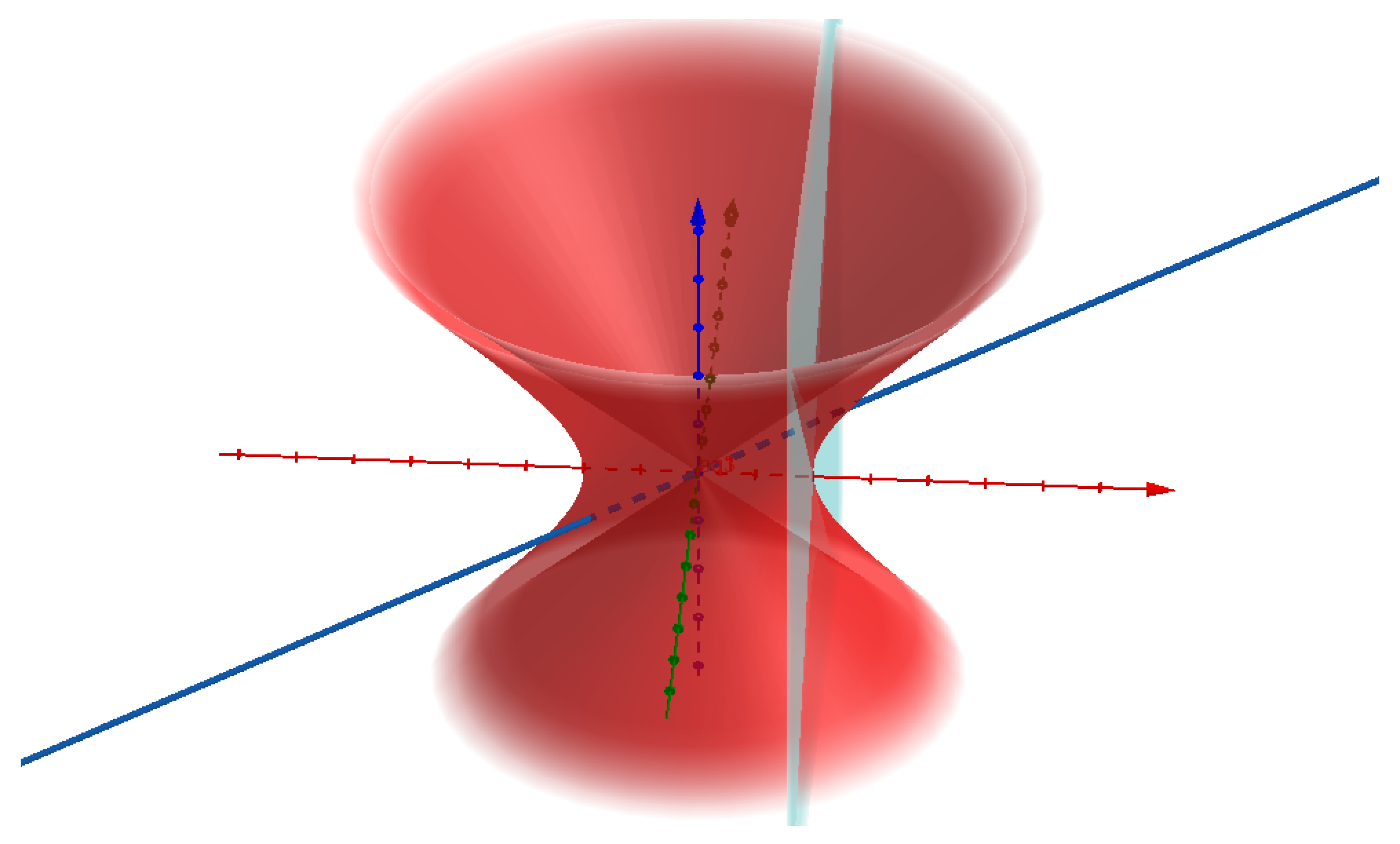
Figure 1.
In a low-dimensional version, the following geometric elements in the five-dimensional Euclidean space are represented: (a) the coordinate axes (x in red, y in green, t in blue); (b) the five-dimensional light-cone with vertex in the origin ; (c) the hyperboloid whose surface is the de Sitter space (in red); (d) the Minkowski space tangent to the hyperboloid (sky blue); (e) a line of gnomonic projection from the origin to the tangent space (blue, dashed) and its extension (blue, solid line).

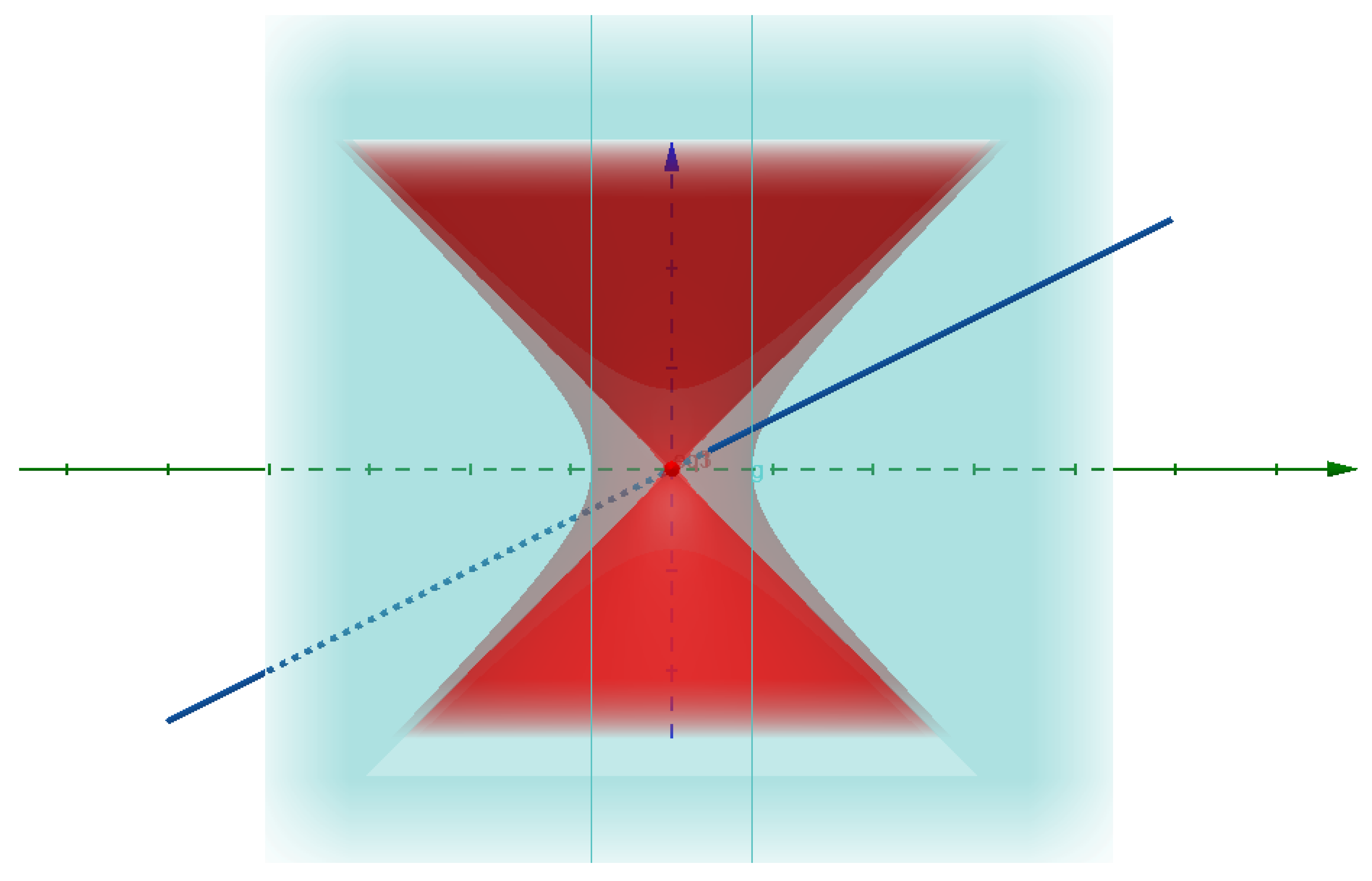
Figure 2.
View of the de Sitter space along the projection line of the tangency point. The five-dimensional light-cone intersects the Minkowski space in a constant proper time hyperbola, whose two sheets are tangent to the surfaces . These latter constitute, together with the lines represented in blue, the de Sitter horizon of the tangency point ( = de Sitter radius).

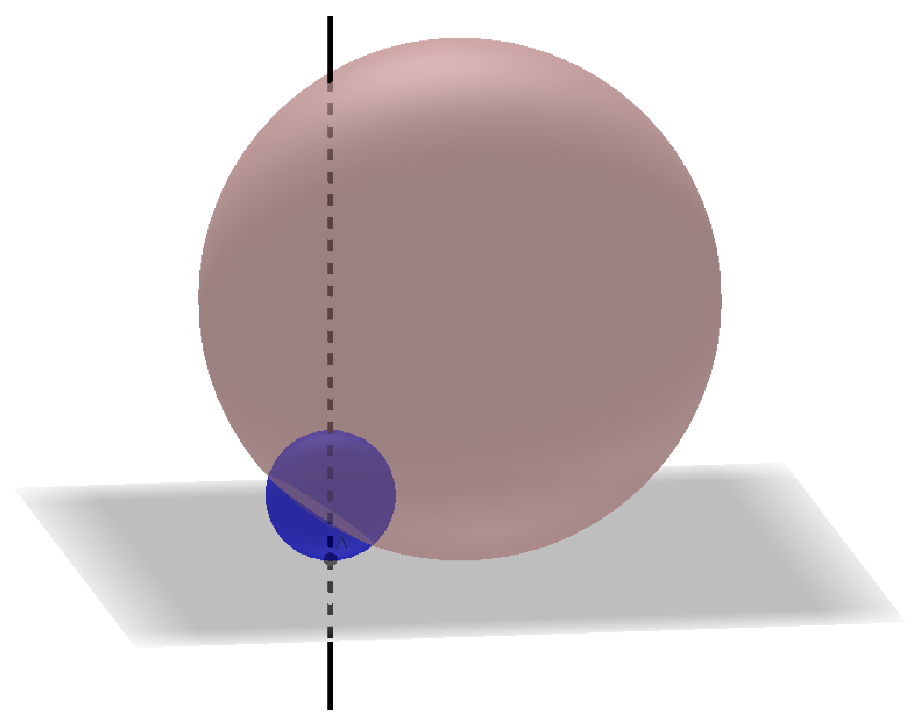
Figure 3.
Both the micro-space of a quark (blue) and that of the hadron to which it belongs (beige) are tangent to the flat Minkowski space. The tangency point of the quark micro-space is confined within the vertical projection of the hadronic micro-space (de Sitter horizon). In five-dimensional space this point is a straight line that intersects the hadronic micro-space in two points. The strong charge of the quark is positioned at one of these two points, while its electric and weak charges are positioned at the point of tangency. The same reasoning applies to gluons. Hence, the strong charges of a hadron are located in a closed space, which is the de Sitter hadronic micro-space. From Gauss theorem it follows that the hadron as a whole is colorless.

Publisher’s Note: MDPI stays neutral with regard to jurisdictional claims in published maps and institutional affiliations. |
© 2020 by the author. Licensee MDPI, Basel, Switzerland. This article is an open access article distributed under the terms and conditions of the Creative Commons Attribution (CC BY) license (http://creativecommons.org/licenses/by/4.0/).
Share and Cite
MDPI and ACS Style
Chiatti, L. Bit from Qubit. A Hypothesis on Wave-Particle Dualism and Fundamental Interactions. Information 2020, 11, 571. https://0-doi-org.brum.beds.ac.uk/10.3390/info11120571
AMA Style
Chiatti L. Bit from Qubit. A Hypothesis on Wave-Particle Dualism and Fundamental Interactions. Information. 2020; 11(12):571. https://0-doi-org.brum.beds.ac.uk/10.3390/info11120571
Chicago/Turabian StyleChiatti, Leonardo. 2020. "Bit from Qubit. A Hypothesis on Wave-Particle Dualism and Fundamental Interactions" Information 11, no. 12: 571. https://0-doi-org.brum.beds.ac.uk/10.3390/info11120571
Note that from the first issue of 2016, this journal uses article numbers instead of page numbers. See further details here.