Multilingual Transformer-Based Personality Traits Estimation


1
Department of Control and Computer Engineering (DAUIN), Politecnico di Torino, Corso Duca degli Abruzzi, 24, 10129 Turin, Italy
2
LINKS Foundation, Via Pier Carlo Boggio, 61, 10138 Turin, Italy
*
Author to whom correspondence should be addressed.
Information 2020, 11(4), 179; https://0-doi-org.brum.beds.ac.uk/10.3390/info11040179
Submission received: 24 January 2020
/
Revised: 19 March 2020
/
Accepted: 21 March 2020
/
Published: 26 March 2020
(This article belongs to the Special Issue Advances in Social Media Analysis)
Abstract
:Intelligent agents have the potential to understand personality traits of human beings because of their every day interaction with us. The assessment of our psychological traits is a useful tool when we require them to simulate empathy. Since the creation of social media platforms, numerous studies dealt with measuring personality traits by gathering users’ information from their social media profiles. Real world applications showed how natural language processing combined with supervised machine learning algorithms are effective in this field. These applications have some limitations such as focusing on English text only and not considering polysemy in text. In this paper, we propose a multilingual model that handles polysemy by analyzing sentences as a semantic ensemble of interconnected words. The proposed approach processes Facebook posts from the myPersonality dataset and it turns them into a high-dimensional array of features, which are then exploited by a deep neural network architecture based on transformer to perform regression. We prove the effectiveness of our work by comparing the mean squared error of our model with existing baselines and the Kullback–Leibler divergence between the relative data distributions. We obtained state-of-the-art results in personality traits estimation from social media posts for all five personality traits.
1. Introduction
Language models have been widely employed to measure personality traits starting from written text. In [1], Frommholz et al. built the Anti Cyberstalking Text-based System (ACTS) to detect cyberstalking in textual contents of social media posts. In parallel, Guntuku et al. used automatic personality trait detection from text to discover social media user depression [2]. In other contexts, personality traits are used to match job candidates and job advertisements, as reported by Neal et al. [3]. In a similar way, IBM developed Personality Insights (https://www.ibm.com/watson/services/personality-insights/). Thanks to this tool, IBM delivered commercial applications that exploit personality traits. As an example, a Japanese airline company improved flight experiences by empowering AI with personality trait assessment skills in their customer communication chatbot (https://www.ibm.com/blogs/client-voices/ai-personalizes-japan-airlines-travel-experience/). These works show how the ability to recognize the semantic meaning of human language led to a fine personality trait measurement. They also detected social risks and they improved user experience. Even if these solutions have a big impact on society, we argue that current techniques do not consider polysemy in text and differences among languages. In fact, they consider each word without its context. The same word could have different meanings in different sentences. These models have another major limitation, namely the focus on only English text. The complexity of languages requires that models represent word meaning in sentences correctly. Furthermore, each culture has a custom set of words representing a specific aspect of the culture itself. These words are not always explainable with an English translation. Thus, we conducted our study answering the following research questions:
- RQ1
- Is sentence encoding based on transformer and deep learning effective in personality trait assessment?
- RQ2
- How do we generalize the model to be multilingual?
In this paper, we present a multilingual transformer-based personality traits estimator that exploits the transformer [4] capabilities of working at sentence level within our deep learning model. We encode sentences into sentence embeddings and then we compute the Big 5 [5] traits (Openness, Conscientiousness, Extraversion, Agreeableness, and Neuroticism) with a supervised approach. Sentences are processed by a specialized transformer encoder that produces a sentence embedding representative of the entire social media post received as input. Our neural network then exploits this sentence embedding to perform a regression on the objective personality trait. Our approach decreases the mean squared error of the actual state of the art measured on the myPersonality gold standard, widely adopted as reference for five factor model trait computation from social media posts. We show that our model has state-of-the-art results with the multilingual model including the Top 104 languages sorted by number of Wikipedia articles in that language. We also checked our model results with using English language alone, obtaining excellent scores. The code we built is available in a publicly accessible repository (https://github.com/D2KLab/SentencePersonality).
The remainder of this paper is structured as follows. In Section 2, we illustrate how various studies approached the problem of personality assessment through machine learning and natural language processing and how our work differs from them and it contributes to the progress in this field, while, in Section 3, we introduce the five factor model, also known as the Big 5 model, a well defined model to compute personality traits. In Section 4, we present the myPersonality gold standard used to compare our results with existing baselines. In Section 5, we explain our approach and we show our neural architecture. In Section 6, we report the experimental results we achieved in personality trait regression when applying our architecture on the myPersonality dataset. In Section 7, we discuss the results obtained with our approach and we explain the choices made for baseline comparison and linguistic model. Finally, we conclude with insights and planned future works in Section 8.
2. Related Work
In the last decade, the estimation of personality traits experienced double-sided progress in terms of linguistic tools and machine learning methods adopted. An exponential interest in the field has been raised from the work of Kosinski et al. [6] since 2013, where they explained the mining of information associated with human personality retrievable from social media platforms. In parallel, 2018 has been a disruptive year in the field of natural language processing because of the BERT model being released by Google [7] that improved the exploitation of latent features in text semantic. We grouped the related works by machine learning category. At the end of this section, we report the studies explaining the use of language to compute personality traits according to the lexical hypothesis.
2.1. Supervised Learning and Personality Traits Estimation
In [8], Carducci et al. created a Support Vector Machine (SVM) to perform a supervised regression with the myPersonality dataset. They developed and fine tuned a SVM with 300-dimensional word embeddings as feature vector and each personality trait score as target. These embeddings are word-based and they are obtained with a query to the pre-trained FastText (https://fasttext.cc/) vocabulary by Facebook. In [9], Quercia et al. performed a regression with myPersonality dataset adopting a supervised approach. They did not adopt linguistic features; instead, their model computes personality traits using the number of following, followers, and listed count. In [10], Alam et al. created an automatic Big 5 personality trait recognition model on Facebook data. They compared various supervised models and selected a Multinomial Naive Bayes (MNB) sparse modeling. They also used linguistic features thanks to a bag-of-words approach and tokens (unigrams) starting from Facebook statuses. These tokens are converted into a vector of features using TF-IDF [11]. In [12], instead, Chaudhary et al. used the Myers–Brigg personality model [13]. They used a Logistic Regression algorithm to classify Myers–Briggs personality type indicator adopting user profile and comments from Kaggle (https://www.kaggle.com/). In [14], Xue et al. created a hierarchical deep neural network, exploiting both convolutional and recurrent models. They worked with the sentence level attention mechanism that considers social media posts not just as a bag of words but as a whole with a technology that concatenates and pools word embeddings. They used doc2vec by Gensim to create document embeddings, while they used a multi-layer perceptron gradient boosted with a SVM to perform and enhance regression on personality trait scores. In [15], Liu et al. built a character to word followed by a word to sentence embedding mechanism to consider the field specific lexicon of social media posts. They exploited the PAN dataset, a collection of tweets from Twitter, and they computed RMSE on each of the five personality traits in the Big 5 model. They built an architecture made of a Char-BiRNN, with Word-Bi-RNN, and then they added a ReLu layer plus a final linear layer to perform regression. They also worked with Spanish and Italian. In [16], Majumder et al. developed a CNN to create a fixed-length feature vector from word2vec word embeddings, which they extended with eighty-four additional features starting from Mairesse’s library [17]. For classification, the so-computed document vectors are fed both to a Multi-Layer Perceptron (MLP) and to a polynomial SVM classifier.
2.2. Unsupervised Learning and Personality Traits Estimation
A different approach emerges from unsupervised learning, because here there is no target feature similar to the myPersonality with questionnaire. In [18], Celli et al. correlated linguistic features, as explained by Mairesse et al. [19], exploiting them with an unsupervised approach, to compute personality traits. As an example, the number of commas inserted in the user text or the number of first person plural pronouns is correlated with a particular personality trait high score. Celli et al. translated the work of Mairesse et al. into features directly retrievable from social media posts. The cited work of Mairesse et al. is not considered unsupervised, but their work and relative findings inspired the subsequent unsupervised approaches. Another unsupervised model developed and applied in [20] exploits Linguistic Inquiry and Word Count (LIWC), software that measures the cognitive and emotional properties of a person. Kafeza et al. used LIWC to understand personality traits in a supervised manner, but then they masked this knowledge to understand which community is the most influential one on Twitter. In [21], Sun et al. created AdaWalk, unsupervised software able to detect personality, and they measured it on a group-level granularity.
2.3. Semi-Supervised Learning and Personality Traits Estimation
In [22], a semi-supervised learning approach is adopted. Bai et al. used the Big Five Inventory (BFI) by Berkeley Personality Lab. It is a self-reported inventory to measure the Big 5 personality dimensions as labeled target. They used the Renren (http://renren.com/) social network to collect data from consensual students at the Graduate University of Chinese Academy of Sciences (GUCAS) to monitor and collect their online behavior. They labeled each interaction on the social network as related to one of the five personality traits in five factor model. In [23], Lukito et al. searched a correlation between personality traits and linguistic choices. They exploited a Twitter dataset geolocalized in Indonesia and they applied Naive Bayes to measure these correlations. They used LIWC for text features extraction. In [24], Iacobelli and Culotta found a correlation between Agreeableness and Emotional Stability (high Emotion Stability means low Neuroticism) applying a conditional random field over the whole five labels of Big 5 model. They considered the labels as binary and not continuous. This methodology is useful to predict structured objects. Their findings suggest that alternative structured approaches have to be taken into consideration while dealing with Big 5 models to enhance the prediction accuracy of a trait, Neuroticism in their case, exploiting the fact that another trait is easier to predict and it is correlated to the former.
2.4. Lexical Hypothesis and NLP in Personality Estimation
The lexical hypothesis motivates the technique to predict personality from the linguistic choices made by a person. This position is supported by many studies on the topic [19,25,26,27,28]. In [29], Kumar et al. extracted the personality traits from written text. They collected a huge text corpus from Facebook, Twitter, and essays correlating the social network structure with personality assessment questionnaires. Concerning the validity of personality trait assessment from text, the work by Pennebaker et al. [25,27] demonstrated this hypothesis. In terms of usefulness of social media in this field, Weisbuch et al. [30] defined and computed the spontaneousness of users in writing social media posts without a deep overthinking about what posting. This finding allows a more effective personality trait computation. Since 2003, algorithms adopted in these fields evolved through years. In [26], Argamon et al. extracted lexical features and they used SVM to make predictions. In details, they used the appraisal lexical taxonomy in Neuroticism detection. This taxonomy follows hierarchical linguistic rules to classify words. The words are related by concepts like hypernymy, synonymy, antonymy, and homonymy. With the wider adoption of deep learning techniques and the incremental availability of data and machine resources, novel studies emerged. In [31], Su et al. used LIWC to make grammar annotations and they applied it with dialogue transcripts. Deep learning methods translate text into a vectorial space through the computation of the word distribution inside textual documents. These numerical arrays gain mathematical properties, such as similarity, available as features to be exploited in model building.
Finally, in [4], Vaswani et al. developed an architecture that is made up of both an encoder and a decoder stack. They maintained both the definition of a word embedding made by its context plus a positional encoding embedding stating the probabilities of each word position. They introduced the concept of attention in word embeddings computation. They mapped a query and a set of key-value pairs to an output. This output is computed as a weighted sum of the values through a compatibility function. In [7], Devlin et al. exploited and adapted the Transformer model to improve word embeddings extraction and deployment when computed at sentence level. They added the concept of masked token to obtain the word embedding of the masked token through a prediction mechanism based on machine learning.
Our work belongs to the category of supervised approaches and it applies the considerations of the lexical hypothesis. In this scenario, we tune and specialize the encoding side of the transformer [4] architecture. We built the encoder as part of our model to extract Big 5 personality traits from social media posts. To improve the sentence representation, we use a special token, as described in Section 5. This choice avoids the pooling phase from word embeddings to sentence embedding that generated an information loss in previous studies. We also create a neural architecture able to perform a regression with a lower mean squared error with respect to other existing models, both supervised and not supervised.
3. Five Factor Personality Model
Among the variety of personality trait assessment models, we decide to use the five factor model one, also known as Big 5 model. The five factor model is a psychometric standard widely adopted. McRae et al. [5] explained how their model integrates many personality constructs efficiently and comprehensively. This model has been corroborated by the works of Tupes and Christal [32], Digman [33], and Goldberg [34].
The personality traits defined by the model are the following:
- Openness to experience (Openness in short) indicates how much a person appreciates new experiences, adventures, or if he is prone to exit his comfort zone.
- Conscientiousness describes the human tendency to be loyal to a schedule, to seek long-term goals, and to be more organized rather than creative or spontaneous.
- Extraversion measures if a person is outgoing and enjoys the companionship of others. A low level in Extraversion means that the candidate prefers to be alone and is reserved.
- Agreeableness tells if people are trusting and altruistic and if they prefer collaboration with respect to competition. A high score in Agreeableness indicates the tendency to maintain positive relationships with others.
- Neuroticism measures emotional stability. It is the only trait that indicates negative emotion when the score is high; in fact, it is often computed in a reverse way and called emotion stability.
These five scores are retrieved through a Likert questionnaire that has a continuous score ranging 1–5, as suggested in the work of McRae and Costa [5]. We focused our work on the methodological and computational part of personality trait prediction. Personality traits as described by McRae and Costa [5] only measure the general attitudes of candidates, but there are further features of personality in the model called facets that we do not compute in this work. Users clustering or other exploitation of these results are beyond the scope of this study.
4. Gold Standard
The myPersonality dataset is the gold standard in personality trait computation for the five factor model (Big 5). Kosinski et al. [6] gathered data of millions of people through their Facebook application. With the consent of candidates using the application, they proposed the assessment of personality traits through a lighter version of the original McRae and Costa NEO-PI-R questionnaire [5]. Each question contributes to the computation of a particular personality trait. As an example of an item in the questionnaire: “Warms up quickly to others”, the user has to answer on a Likert scale in the range 1–5, from disagree strongly to agree strongly. In this case, the answer given contributes to the definition of the Extraversion personality trait of the tested candidate. The myPersonality dataset also collects Facebook posts of users and it couples them with their personality questionnaire results. We worked on a subset of the whole dataset made of 9913 samples defined as myPersonality small. We used two files in the dataset: in the first one, each line is made up of a message id, a user id, the plain text of message (social media post), and other information; in the second file, each line contains the user id and the five personality trait scores associated with the user id i in the range 1–5. The file status_update.csv contains the message id, the user id, the raw text of the message, last updated_time, and nchar length of the message. As an example, the first line is:
1,d2504ff7e14a20d0bb263e82b77622e7,"is very well rested. Off to starbucks to catch up with a friend.",2009-06-15 14:47:52,67
In the file big5.csv, we find the user id, the five personality trait scores for that user, the item_level, blocks, and date. As an example, the first line is:
605ff548660b7ed55d519b0058b9649e,4.20,4.50,4.25,3.15,2.05,1,336,2009-05-14
The myPersonality dataset contains data collected from 2007 to 2012. This Facebook application also collected the whole information related to the Facebook profile of the user answering the questionnaire, again asking to users their consent. From 2018, this dataset is no longer available according to what reported by Kosinski on the webpage of the project (https://sites.google.com/michalkosinski.com/mypersonality).
In Figure 1, we show the frequency of the five personality trait questionnaire results (Openness, Conscientiousness, Extraversion, Agreeableness, and Neuroticism) from the myPersonality dataset.
5. Approach and Contribution
We created a linguistic model based on a sentence level attention mechanism enhanced by a neural network architecture that performs a continuous regression. The myPersonality dataset provides the gold standard on which we tested our model and we compared it with existing baselines. We improve the social media user personality prediction having as sole information the text posted on Facebook. In the following, we outline how we processed the input text and how we developed the stacked neural network for each of the five personality traits. A stacked neural network is defined as a combination of publicly available neural network architectures whose features are extracted at an intermediate layer of the network, and then concatenated together to form a larger feature set.
5.1. Sentence Embeddings with Transformer
We performed the analysis on a dataset made of social media posts in textual format. When the text is given as input in our processing pipeline, as shown in Figure 2, it is in its raw format because we want to preserve the meaning expressed by the original social media author. According to this consideration, text cleaning is not performed, with the exception of @, http, and punctuation removal. The BERT-tokenizer splits sentences into words and then into sub-strings to handle out of vocabulary words. Due to our social media context, we used spacymoji (https://pypi.org/project/spacymoji/) to consider also emoticons. We translate the graphical representation of emoticons into their textual descriptions, for examples:
- 😊 becomes smiling face with smiling eyes; and
- 👍 becomes thumbs up.
Each sentence from myPersonality is represented as a list of tokens after the initial tokenization phase. Once split, we add a special token (CLS stands for classification and it is trained as a custom token in the model) to perform sentence classification at the beginning of the token list. It is important to notice that we use the embedding of the CLS token to perform a regression task. The CLS syntax is adopted in the BERT [7] architecture to diversify among different tasks. One of these tasks is to associate labels to this special token trained with the Transformer architecture and the attention mechanism as described in [4]. The CLS token avoids the need for sum, max, min, and concatenation of word embeddings at the end of the encoding phase. This behavior transfers the problem from a word based mechanism to a sentence level one. At the end of each sentence, we add another special token (SEP stands for separator) also trained as a custom token in the model. Then, we exploit the BERT positional embeddings and the successive twelve encoding layers to generate a word embedding for each token, as described by Devlin et al. [7]. The first encoding layer is represented in Figure 3. The other eleven encoding layers have the same representation, but instead of word embeddings retrieved from WordPiece vocabulary after tokenization, they receive as input the embeddings obtained after self-attention and feed-forward processing in the previous layer. At the end of this phase, we delete all the embeddings except the CLS one or sentence embedding. The sentence embedding is computed considering the surrounding context, in this case the entire sentence, thus we select it as representative of the sentence as a whole. A single token has 768 dimensions, following the optimal configuration of the BERT base model [7]. The number 768 comes from the empirical experiment reported in [7], where the authors suggested it as the best number of features comparing the obtained results in different tasks: GLUE, SQuAD, NER, and MLNI. Thanks to the sentence embedding, we do not need pooling (as we explain in Section 7) or other forms of aggregation between the word embeddings of the single words in the sentence, but we directly perform the following operations on this 768 dimensional array. Figure 4 illustrates the text processing steps, from input tokenization to word embedding and eventually the sentence embedding. The encoder architecture, illustrated in Figure 4, is an optimized and lighter version of BERT. It is specialized in sentence encoding, as described in Section 6. We derive the architecture by the bert-as-a-service library (https://github.com/hanxiao/bert-as-service). The parameters in the tokenization phase are described in Section 5.3 and the choices made are listed in Table 1. The choice behind the sentence level attention mechanism originates from the assumption that a single word used in different contexts cannot be represented with the same word embedding. This situation is called polysemy in text and the challenge to be solved is the Winograd Schema Challenge (WSC) (http://commonsensereasoning.org/winograd.html). This sentence was given by Hector Levesque in 2011 as an example: The trophy would not fit in the brown suitcase because it was too big. The reader knows what was too big, but for an intelligent agent it is not easy. The other situation where polysemy in text needs to be addressed is in sentences such as the one reported by Google (https://ai.googleblog.com/2017/08/transformer-novel-neural-network.html): “I arrived at the bank after crossing the...” requires knowing if the sentence ends in “... road.” or “... river.” Sentence level attention mechanism is suited to our scenario, where each word is relevant for the social media post understanding. In particular, we have medium and short sentences, thus the weight of each word is greater in this context. We must consider precisely each word to catch the meaning of the sentence and to predict the personality trait scores associated with the sentence with an error as small as possible.
5.2. Stacked Neural Network
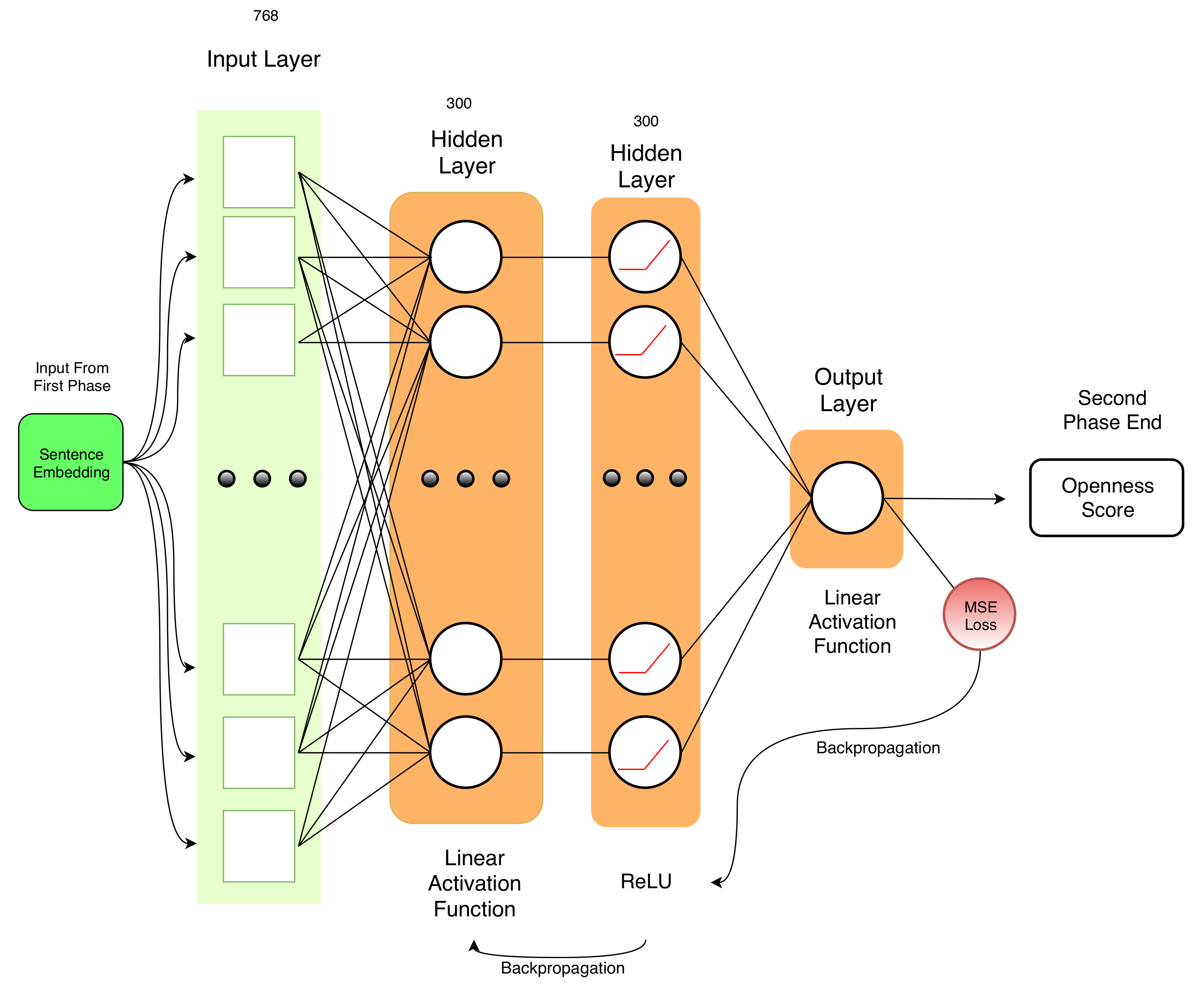
The stacked neural network, illustrated in Figure 5, represents our main contribution. It allows us to define a new state of the art in personality trait prediction from text. As shown in Section 6, we reduce significantly the mean squared error in trait prediction and we also create a smoother data distribution of the predicted scores. In fact, the scores at the tails of the data distribution are detected more correctly than previous models [6,8,9]. Our stacked neural network receives as input the 768-dimensional CLS token from the encoding phase in our pipeline, as illustrated in Figure 2. Then, with a linear activation function in a feed-forward layer, we reduce the dimensionality of the input to 300 dimensions. We adopt the same architecture for each of the five personality traits (Openness, Conscientiousness, Extraversion, Agreeableness, and Neuroticism).
The work and analysis of Carducci et al. [8] and Landauer and Dumais [35] suggested 300 as the ideal number of features in personality traits estimation. They discovered with empirical experiments that 300 features represent a word distribution in an optimal way. We tried many configurations of the number of neurons of this hidden layer, but when experimenting with more than 300 neurons we improved neither the execution time nor the mean squared error. The following layer performs a ReLu, as in Equation (2), that is an activation function in each neuron. This choice improves the performance and it speeds up the learning phase. It is also used to avoid the vanishing gradient problem. We have a vanishing gradient in feed-forward network when we back-propagate the error signal and it decreases/increases exponentially with respect to the distance from the final layer. Finally, there is a layer with a single neuron that uses a linear activation function to perform the regression. The regression predicts one of the five personality traits starting from the initial vector , where . We decided to use the linear function to represent , where represents the linear function family parameterized by . We search the that minimizes Equation (1), our objective function.
5.3. Model Optimization
Hyper-parameters must be defined both for the encoding phase and the regression phase architectures. In Table 1, regarding the architecture of Figure 4, we set these parameters:
- Hidden Size is the number of neurons in each hidden layer.
- Hidden Layers is the number of layers represented with the self-attention plus feed-forward.
- Attention Heads is the number that tunes the self-attention mechanisms described in the work of Vaswani et al. [4].
- Intermediate Size represents the number of neurons in the inner neural network of the encoder feed-forward side.
- Hidden Activation Function t is the non-linear activation function in the encoder. GeLu is the Gaussian Error Linear Unit.
- Dropout Probability is the probability of training a given node in a layer where 0 is no training and 1 always trained.
- Maximum Position Embedding is the maximum sequence length accepted by the model.
As additional parameters, we define pooling_strategy as CLS_TOKEN, meaning not to use any pooling strategy and to create a CLS token at the beginning of the list of tokens of each sentence, respectively.
On the other side, as shown in Table 2, we also have to optimize our neural network architecture with the following parameters:
- Optimizer changes the weights of the neurons based on loss to obtain the most accurate result possible.
- Learning Rate is the correction factor applied to decrease the loss. Too high values of learning rate lose some details in weights setting, while too low values may lead the model to a very slow convergence.
- Loss Function computes the distance between predicted values and actual values.
- Batch Size is the number of training examples utilized in one iteration.
The parameters chosen in our neural network architecture are listed in Table 2. The choices we made were validated empirically.
6. Experimental Results
To assess that our model is improving on the actual state of the art, we compared it with previous models as well as different configurations of the encoding and regression stages. The experiment was performed on the myPersonality small dataset (9913 records).
In Table 3, we compare our results with the existing baselines in terms of mean squared error. We chose the mean squared error because it is more sensitive to not uniform large variation in error than Mean Absolute Error (MAE). In the context of personality trait prediction, we must accept light variations between predicted and actual scores. However, we must immediately spot huge mis-predictions even in few cases. MSE increases not only with the variance of the errors, but also with the variance of the frequency distribution of error magnitudes. Furthermore, we selected MSE because we compared our model with the previous ones in this field that used MSE. Instead, we do not report R-squared because all the baselines used for comparisons do not report this information.
In Table 3 we compare actual state of the art by Carducci et al. [8], with the results obtained by Quercia et al. [9] and with three different configurations of our model. The line labeled as Transformer + SVM shows the MSE obtained with the encoding phase of Figure 4 and then applying a SVM to perform the regression. In this case, none of the MSE obtained improved the state of the art, meaning that just the encoding phase alone is necessary but not sufficient to predict the personality traits better. The row FastText + NN shows the results adopting the word level encoding mechanism with pre-trained word embeddings from FastText (https://fasttext.cc/docs/en/english-vectors.html) and then applying our stacked neural network, as shown in Figure 5. In this scenario, we improved the state of the art for only three traits out of five traits (CON, EXT, and AGR), as we do not represent well enough Openness and Neuroticism. These MSE scores show how our model is able to leverage latent features also from a word level text encoding but it needs more information to exploit its full potential with all personality traits. Finally, the enhancement introduced by the sentence level attention mechanism in the text encoding combined with the neural network is able to outperform the actual state of the art on all the five traits.
Model Verification and Baselines Comparison
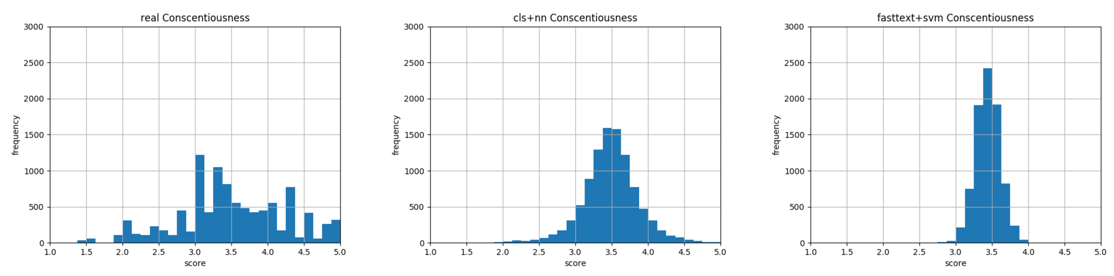
The histograms in Figure 6, Figure 7, Figure 8, Figure 9 and Figure 10 show data distribution of personality traits obtained with questionnaire in myPersonality small on the left figures, our predictions in the central figures and predictions of personality traits obtained with the model by Carducci et al. [8] in the right figures. Nonetheless, we validated our result with the MSE in Table 3. In all the central figures, our model computes the personality traits still following a Gaussian shape, but it is more capable than the model by Carducci et al. [8] to represent values at the margin of the range 1–5 given by the results of a personality trait assessment. On the left of each triplet, there are histograms relative to the personality traits computed through the personality test. These figures show how real values tend to be equally represented; instead, our automatic prediction from text analysis still follows a different shape. Nevertheless, the choice we made went to the right direction to a nearer to truth computation of the personality traits than the current state of the art.
Kullback–Leibler divergence [36], defined in Equation (4), is a measure of how well a probability distribution Q is efficient or not to approximate the true probability distribution P. In fact, we expect to predict personality traits from text as strict as possible to the personality traits obtained through the psychological test. In this sense, we must see our results approximating the real ones. Equation (8) is the KL divergence expressed in the form of a discrete summation. Equation (6) defines the entropy of P used in Equation (4). A low entropy is a measure of a high predictability of information contained in P. In Equation (5), cross-entropy measures the distance between what the true distribution is representing and how well it is represented by the approximating distribution. In Table 4, Table 5, Table 6, Table 7 and Table 8, we consider the first column as the Q probability distributions and the first line as the P probability distributions with respect to the order shown by Equation (4). We specify this because KL is not commutative. These results show how our model is the most efficient in approximating personality trait distribution obtained from questionnaire in Neuroticism, Extraversion, and Openness traits. With these results, we answer the first research question. In fact, we reduced the existing error in automatic personality trait assessment from written text by creating a pipeline, shown in Figure 2, made of an encoder and a neural architecture. In conclusion, sentence encoding with transformer and deep learning are effective in the field of personality trait assessment. The entire pipeline that solved this issue is illustrated in Figure 2, while the encoder phase is in Figure 4 and the regression phase is in Figure 5.
We answered the second research question with a multilingual model (https://storage.googleapis.com/bert_models/2018_11_23/multi_cased_L-12_H-768_A-12.zip). It is important to notice that the model is not cross-lingual because it deals with one language at a time. If the sentence to process contains, for example, Spanish, French, and Chinese words mixed together, the model is not able to perform the regression correctly. We performed the regression with sentences made of words from one language at a time. The dataset adopted for the multilingual configuration is the myPersonality small described in Section 4.
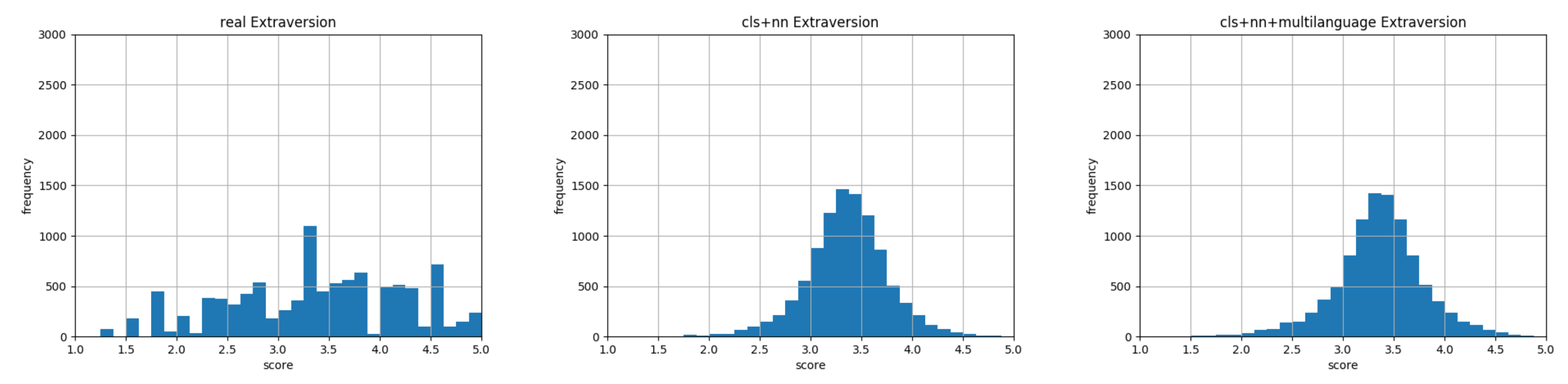
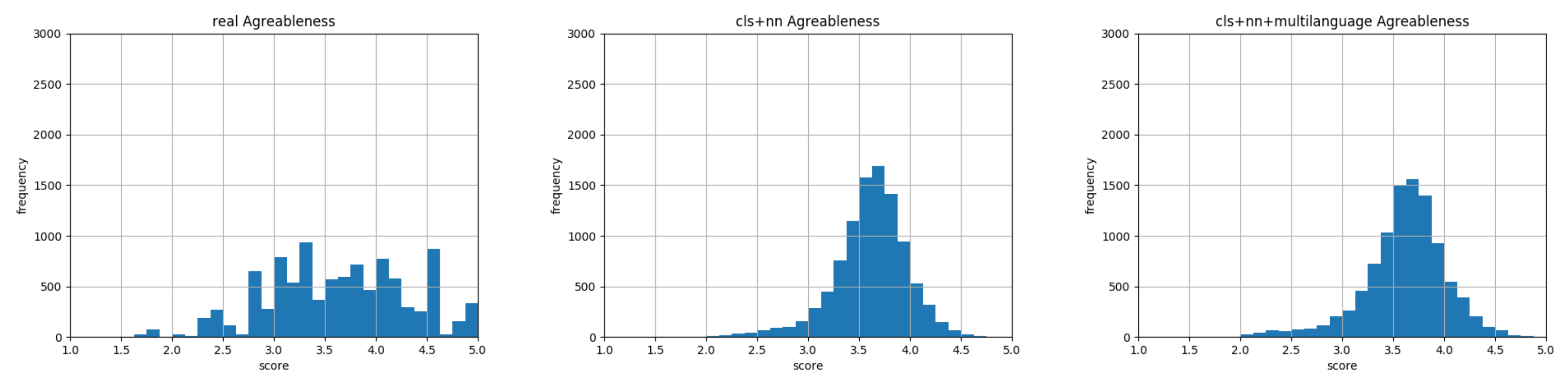
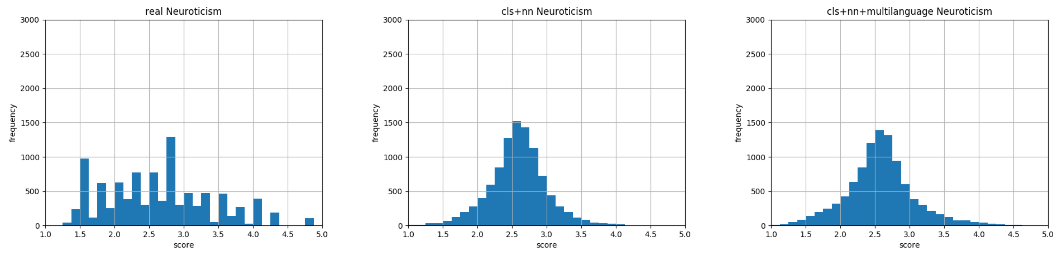
This multilingual model was trained on 104 languages (https://github.com/google-research/bert/blob/master/multilingual.md#list-of-languages). This multilingual model is able to compute word embeddings of 104 different languages. Starting from these embeddings, we performed the regression as described in Section 5. As shown in Figure 11, Figure 12, Figure 13, Figure 14 and Figure 15, the shape of the predicted data distribution multilingual model follows the one created with the predicted English one. To detect an effective improvement in results obtained, we must look at the MSE in Table 3 and at the KL divergence between them in Table 9. The data highlight that, with a model able to understand 104 languages, we reduced the mean squared error and we approximated the data distribution of the myPersonality dataset in a more efficient way. In conclusion, we answered to the second research question by choosing a sentence embedding model trained on a multilingual environment and by changing this element in the encoding phase of our pipeline (Figure 2).
7. Discussion
In Section 6, we use the mean squared error reported in Table 3 to show that our results outperformed the current state-of-the art. We obtained an average improvement of 30% over each of the five personality traits. We addressed the lack of discriminative power problem of previous systems. This outcome is visible in Figure 6, Figure 7, Figure 8, Figure 9 and Figure 10, where the scores at the tails of the range 1–5 are more represented; in this sense, our model is more discriminative. This achievement is further described by the Kullback–Leibler divergence in Table 4, Table 5, Table 6, Table 7 and Table 8, where we highlight how efficient is our model to approximate the real data distribution through predicted data. Nevertheless, the histograms also highlight the remaining margin of improvement. In fact, our data distribution still tends to follow a Gaussian shape, because the target of the mean squared error reduction tends to predict scores closer to the center of the interval. Due to this evidence, we must further expand the neural network or tweak the encoding phase to better describe and exploit the latent features. We only used raw text from the myPersonality dataset to allow an easier transfer learning environment. Social media posts in the form of plain text are more accessible than other personal and private information. Our solution with just raw text is working, but further analysis is needed with additional features. Furthermore, we operated at single post level and not at a user-wise level, both for results obtained and to remove the strict correlation of personality traits as fixed in time. This means that a single user will obtain different personality trait scores depending on the content he writes. Another focus of our work is on the avoidance of a pooling system in the context of word embeddings due to the choice of working at sentence level. This passage is clarified in Figure 4, when we choose CLS token instead of performing pooling among every word embedding of the sentence analyzed. In addition, this choice is visible in our repository in the file create_train_table_whole_lines.py when pooling strategy is set to CLS_TOKEN. This choice is fundamental because it allows us not to lose information when averaging, summing, or concatenating word embeddings, thus not impoverishing the knowledge obtained that must be used to make a better prediction of traits during the regression phase. The assessment of personality traits has been deployed for commercial usage by IBM through the product called IBM Personality Insights (https://www.ibm.com/watson/services/personality-insights/). IBM adopts various models, and five factor model is one of them. We compared their prediction of personality traits of myPersonality dataset, using their API, with ours, as shown in Table 3. The scores obtained with IBM Personality Insights are lower than ours, but, due to constraints on number of words in the API, it operates at user level, grouping all social media posts of each user in each query to input enough text. IBM states that the model they built needs at least a few hundred words to compute personality traits, otherwise the predictions made are meaningless.
8. Conclusions and Future Work
We describe a model to process social media posts, encoding each of them on a sentence level into a high-dimensional array space. We processed this array of 768 features with a stacked neural network to perform a regression on each of the five personality traits in the Big 5 model (Openness, Extraversion, Agreeableness, Conscientiousness, and Neuroticism). Our model is the same for all five personality traits, but it computes them separately, tuning different weights per personality trait. We worked in a supervised environment, where expected personality traits are numbers in the continuous range 1–5 and we predicted them just looking at the textual content of each social media post. The target features came from the myPersonality gold standard. The obtained results have a lower the mean squared error with respect to the existing state of the art. They were also confirmed by the Kullback–Leibler divergence in the data distribution. These results were obtained with a multilingual model that understands 104 languages and then reproduced with the English text only. The code we built is available in a publicly accessible repository (https://github.com/D2KLab/SentencePersonality). Apart from improving the model and testing with different data sources, such as PAN-AP-15 dataset [37] and that of Rangel et al. [38], we plan further studies in this field. We want to measure the impact of our work when applied with conversational agents and virtual assistants. We plan to experiment on a longer span of time to monitor and understand if and how the personality traits of experiment candidates change. We will tune the answer of conversational agents based on human personality traits. We want to compute them in real time during the dialogue to improve the digital experience in terms of recommendation received and empathy. We aim to encourage serendipity and creativity with this approach. We are also studying the weight of personality traits on the production of viral contents and how to apply it for promoting positive behaviors and for disseminating verified scientific news. We want to build a tool to remove emotions and personality traits from newspaper articles to enhance the objectivity of the fact against the personal opinion of the writer. We aim to build empathetic conversational agents that grow side by side with the user becoming proactive in the conversation and not just passive in questions answering or in command execution. In this scenario, the agent builds its behavior learning from the user it is assisting.
Author Contributions
Conceptualization, S.L., D.M., and G.R.; investigation, S.L.; methodology, S.L. and D.M.; project administration, M.M.; software S.L. and D.M.; supervision, G.R. and M.M.; validation, D.M. and G.R.; visualization, S.L.; writing—original draft, S.L.; and writing—review and editing, D.M., G.R. and M.M. All authors have read and agreed to the published version of the manuscript.
Funding
This research received no external funding.
Acknowledgments
A special thanks is given to the myPersonality project for having shared with us the dataset used for training our learning model and conducting the experimentation. Computational resources were provided by HPC@POLITO, a project of Academic Computing within the Department of Control and Computer Engineering at the Politecnico di Torino (http://www.hpc.polito.it).
Conflicts of Interest
The authors declare no conflict of interest.
Abbreviations
The following abbreviations are used in this manuscript:
| MSE | Mean Squared Error |
| SVM | Support Vector Machines |
| NN | Neural Network |
| OPE | Openness |
| CON | Conscientiousness |
| EXT | Extraversion |
| AGR | Agreeableness |
| NEU | Neuroticism |
| NLP | Natural Language Processing |
| KL | Kullback–Leibler |
References
- Frommholz, I.; Al-Khateeb, H.M.; Potthast, M.; Ghasem, Z.; Shukla, M.; Short, E. On Textual Analysis and Machine Learning for Cyberstalking Detection. Datenbank-Spektrum 2016, 16, 127–135. [Google Scholar] [CrossRef] [Green Version]
- Guntuku, S.C.; Yaden, D.B.; Kern, M.L.; Ungar, L.H.; Eichstaedt, J.C. Detecting Depression and Mental Illness on Social Media: An Integrative Review. Curr. Opin. Behav. Sci. 2017, 18, 43–49. [Google Scholar] [CrossRef]
- Neal, A.; Yeo, G.; Koy, A.; Xiao, T. Predicting the Form and Direction of Work Role Performance from the Big 5 Model of Personality Traits. J. Organ. Behav. 2012, 33, 175–192. [Google Scholar] [CrossRef]
- Vaswani, A.; Shazeer, N.; Parmar, N.; Uszkoreit, J.; Jones, L.; Gomez, A.N.; Kaiser, L.; Polosukhin, I. Attention Is All You Need. arXiv 2017, arXiv:1706.03762v5. [Google Scholar]
- McCrae, R.R.; Costa, P.T. Empirical and Theoretical Status of the Five-Factor Model of Personality Traits. In The SAGE Handbook of Personality Theory and Assessment: Volume 1—Personality Theories and Models; SAGE Publications Ltd.: Los Angeles, CA, USA, 2008; pp. 273–294. [Google Scholar] [CrossRef]
- Kosinski, M.; Stillwell, D.; Graepel, T. Private Traits and Attributes Are Predictable from Digital Records of Human Behavior. Proc. Natl. Acad. Sci. USA 2013, 110, 5802–5805. [Google Scholar] [CrossRef] [PubMed] [Green Version]
- Devlin, J.; Chang, M.W.; Lee, K.; Toutanova, K. BERT: Pre-training of Deep Bidirectional Transformers for Language Understanding. arXiv 2018, arXiv:1810.04805. [Google Scholar]
- Carducci, G.; Rizzo, G.; Monti, D.; Palumbo, E.; Morisio, M. TwitPersonality: Computing Personality Traits from Tweets Using Word Embeddings and Supervised Learning. Information 2018, 9, 127. [Google Scholar] [CrossRef] [Green Version]
- Quercia, D.; Kosinski, M.; Stillwell, D.; Crowcroft, J. Our twitter profiles, our selves: Predicting personality with twitter. In Proceedings of the 2011 IEEE Third International Conference on Privacy, Security, Risk and Trust and 2011 IEEE Third International Conference on Social Computing, Boston, MA, USA, 9–11 October 2011; pp. 180–185. [Google Scholar]
- Alam, F.; Stepanov, E.A.; Riccardi, G. Personality Traits Recognition on Social Network—Facebook. In Proceedings of the Seventh International AAAI Conference on Weblogs and Social Media, Cambridge, MA, USA, 8–11 July 2013. [Google Scholar]
- Manning, C.D.; Raghavan, P.; Schütze, H. Introduction to Information Retrieval; Cambridge University Press: Cambridge, UK, 2008. [Google Scholar]
- Chaudhary, S.; Sing, R.; Hasan, S.T.; Kaur, I. A comparative Study of Different Classifiers for Myers-Brigg Personality Prediction Model. IRJET 2018, 5, 1410–1413. [Google Scholar]
- Briggs, K.C. Myers-Briggs Type Indicator; Consulting Psychologists Press: Palo Alto, CA, USA, 1976. [Google Scholar]
- Xue, D.; Wu, L.; Hong, Z.; Guo, S.; Gao, L.; Wu, Z.; Zhong, X.F.; Sun, J. Deep Learning-based Personality Recognition from Text Posts of Online Social Networks. Appl. Intell. 2018, 48, 4232–4246. [Google Scholar] [CrossRef]
- Liu, F.; Nowson, S.; Perez, J. A Language-independent and Compositional Model for Personality Trait Recognition from Short Texts. arXiv 2016, arXiv:1610.04345. [Google Scholar]
- Majumder, N.; Poria, S.; Gelbukh, A.; Cambria, E. Deep Learning-Based Document Modeling for Personality Detection from Text. IEEE Intell. Syst. 2017, 32, 74–79. [Google Scholar] [CrossRef]
- Mikolov, T.; Chen, K.; Corrado, G.; Dean, J. Efficient Estimation of Word Representations in Vector Space. arXiv 2013, arXiv:1301.3781. [Google Scholar]
- Celli, F. Unsupervised Personality Recognition for Social Network Sites. In Proceedings of the Sixth International Conference on Digital Society, Valencia, Spain, 30 January–4 February 2012. [Google Scholar]
- Mairesse, F.; Walker, M.A.; Mehl, M.R.; Moore, R.K. Using Linguistic Cues for the Automatic Recognition of Personality in Conversation and Text. J. Artif. Intell. Res. 2007, 30, 457–500. [Google Scholar] [CrossRef]
- Kafeza, E.; Kanavos, A.; Makris, C.; Vikatos, P. T-PICE: Twitter Personality Based Influential Communities Extraction System. In Proceedings of the 2014 IEEE International Congress on Big Data, Anchorage, AK, USA, 27 June–2 July 2014. [Google Scholar] [CrossRef]
- Sun, X.; Liu, B.; Meng, Q.; Cao, J.; Luo, J.; Yin, H. Group-level Personality Detection Based on Text Generated Networks. World Wide Web 2019. [Google Scholar] [CrossRef]
- Bai, S.; Zhu, T.; Cheng, L. Big-Five Personality Prediction Based on User Behaviors at Social Network Sites. arXiv 2012, arXiv:1204.4809. [Google Scholar]
- Lukito, L.C.; Erwin, A.; Purnama, J.; Danoekoesoemo, W. Social Media User Personality Classification Using Computational Linguistic. In Proceedings of the 2016 8th International Conference on Information Technology and Electrical Engineering (ICITEE), Yogyakarta, Indonesia, 5–6 October 2016; pp. 1–6. [Google Scholar] [CrossRef]
- Iacobelli, F.; Culotta, A. Too Neurotic, Not too Friendly: Structured Personality Classification on Textual Data. In Proceedings of the Seventh International AAAI Conference on Weblogs and Social Media, Boston, MA, USA, 8–11 July 201.
- Pennebaker, J.W.; King, L.A. Linguistic Styles: Language Use as an Individual Difference. J. Personal. Soc. Psychol. 1999, 77, 1296. [Google Scholar] [CrossRef]
- Argamon, S.; Dhawle, S.; Koppel, M.; Pennebaker, J.W. Lexical Predictors of Personality Type. In Proceedings of the 2005 Joint Annual Meeting of the Interface and the Classificaton Society of North America, Cincinnati, OH, USA, 8–12 June 2005. [Google Scholar]
- Pennebaker, J.W.; Mehl, M.R.; Niederhoffer, K.G. Psychological Aspects of Natural Language Use: Our words, our selves. Annu. Rev. Psychol. 2003, 54, 547–577. [Google Scholar] [CrossRef] [Green Version]
- Oberlander, J.; Gill, A.J. Language with Character: A Stratified Corpus Comparison of Individual Differences in e-mail Communication. Discourse Process. 2006, 42, 239–270. [Google Scholar] [CrossRef]
- Kumar, U.; Reganti, A.N.; Maheshwari, T.; Chakroborty, T.; Gambäck, B.; Das, A. Inducing Personalities and Values from Language Use in Social Network Communities. Inf. Syst. Front. 2018, 20, 1219–1240. [Google Scholar] [CrossRef]
- Weisbuch, M.; Ivcevic, Z.; Ambady, N. On Being Liked on the Web and in the “Real World”: Consistency in First Impressions across Personal Webpages and Spontaneous Behavior. J. Exp. Soc. Psychol. 2009, 45, 573–576. [Google Scholar] [CrossRef] [Green Version]
- Su, M.; Wu, C.; Zheng, Y. Exploiting Turn-Taking Temporal Evolution for Personality Trait Perception in Dyadic Conversations. IEEE/ACM Trans. Audio Speech Lang. Process. 2016, 24, 733–744. [Google Scholar] [CrossRef]
- Tupes, E.C.; Christal, R.E. Recurrent Personality Factors Based on Trait Ratings. J. Personal. 1992, 60, 225–251. [Google Scholar] [CrossRef] [PubMed]
- Digman, J.M. Personality Structure: Emergence of the Five-factor Model. Annu. Rev. Psychol. 1990, 41, 417–440. [Google Scholar] [CrossRef]
- Goldberg, L.R. The Structure of Phenotypic Personality Traits. Am. Psychol. 1993, 48, 26. [Google Scholar] [CrossRef] [PubMed]
- Landauer, T.K.; Dumais, S.T. A solution to Plato’s problem: The latent semantic analysis theory of acquisition, induction, and representation of knowledge. Psychol. Rev. 1997, 104, 211. [Google Scholar] [CrossRef]
- Joyce, J.M. Kullback-Leibler Divergence. In International Encyclopedia of Statistical Science; Springer: Berlin/Heidelberg, Germany, 2011; pp. 720–722. [Google Scholar] [CrossRef]
- Rangel Pardo, F.M.; Celli, F.; Rosso, P.; Potthast, M.; Stein, B.; Daelemans, W. Overview of the 3rd Author Profiling Task at PAN 2015. In Proceedings of the CLEF 2015 Labs and Workshops, Notebook Papers, Toulouse, France, 8–11 September 2015; pp. 1–8. [Google Scholar]
- Rangel, F.; Rosso, P.; Verhoeven, B.; Daelemans, W.; Potthast, M.; Stein, B. Overview of the 4th author profiling task at PAN 2016: Cross-genre evaluations. In Proceedings of the CEUR Workshop of Working Notes of the CLEF 2016 Evaluation Labs, Évora, Portugal, 5–8 September 2016; pp. 750–784. [Google Scholar]
Figure 1.
Openness, Conscientiousness, Extraversion, Agreeableness, and Neuroticism of the gold standard. OPE = Openness; CON = Conscientiousness; EXT = Extraversion; AGR = Agreeableness; NEU = Neuroticism. The first three traits are indices of people’s preferences toward new experience, strict deadlines, and well defined goals and ability to be extroverted with scores near to 5, and vice versa for low scores. The last two traits are indices of human predilection toward altruism and low resistance under pressure with scores near to 5, and vice versa for low scores. The myPersonality small contains 9913 records. In these figures, on the horizontal axis is the 1–5 continuous range of personality trait score as computed by the Big 5 model. We grouped scores in discrete ranges to obtain a clear and readable graphic. On the vertical axis is the frequency of the scores present in myPersonality small. Even with the questionnaire results based on the answers of candidates there are some peaks in each of the figures. This is an index that personality traits tend to be more represented in certain score ranges.

Figure 2.
The pipeline representing the whole process from raw text through sentence encoding and then the stacked neural network to predict the personality trait. As shown in the figure, we compute one personality trait out of the five in the Big 5 model. The same pipeline is adopted to compute one by one each of the five personality traits.

Figure 3.
This is a representation of one encoding layer mentioned in Figure 4. There are twelve of this encoding layer in the final architecture. The word embedding of each token passes through these encoding layers and at the end we obtain the transformed word embeddings.
Figure 3.
This is a representation of one encoding layer mentioned in Figure 4. There are twelve of this encoding layer in the final architecture. The word embedding of each token passes through these encoding layers and at the end we obtain the transformed word embeddings.

Figure 4.
Tokenization and encoding with transformer. Each sentence in myPersonality dataset is processed as shown in figure. After punctuation removal, we add CLS token (classification task special token pre-trained in BERT model as a custom token) at the beginning of the sentence and the SEP token (separation between sentences, pre-trained in BERT model as a custom token) at the end of the sentence. We then split the sentence into tokens. The model is able to consider also out of vocabulary words by splitting them into sub-tokens. The second part of the split words is preceded by ## to tag it as a not standalone word. Tokens are mapped into id contained in the WordPiece vocabulary and the array so-computed is transformed into a tensor. We also need a tensor with the same length of token_ids tensor, called segments_ids tensor made of 1s. The segments_ids is useful to divide tokens belonging to the first sentence (0s) to the second one (1s) when we perform a task that needs two sentences, for example question answering or next sentence prediction. In our case, we need just a sentence, so we load segments_ids with 1s. We load pretrained embeddings from BERT model to output word embeddings from our tensors and we add to them to an initially random positional embeddings. At the bottom of the figure, there are twelve encoding layers having a self attention and a feed forward network inside that encode the input into the final sentence embedding.

Figure 5.
Stacked neural network. Starting from the sentence embedding from the encoding phase, we build a stacked model with two hidden layers with, respectively, a linear activation function in each neuron and then a ReLu. The output layer performs the regression on the personality trait score.
Figure 5.
Stacked neural network. Starting from the sentence embedding from the encoding phase, we build a stacked model with two hidden layers with, respectively, a linear activation function in each neuron and then a ReLu. The output layer performs the regression on the personality trait score.

Figure 6.
Openness: Histograms representing data distribution of gold standard on the left, our model result in the middle, and previous state of the art by Carducci et al. [8] on the right.
Figure 6.
Openness: Histograms representing data distribution of gold standard on the left, our model result in the middle, and previous state of the art by Carducci et al. [8] on the right.

Figure 7.
Conscientiousness: Histograms representing data distribution of gold standard on the left, our model result in the middle, and previous state of the art by Carducci et al. [8] on the right.
Figure 7.
Conscientiousness: Histograms representing data distribution of gold standard on the left, our model result in the middle, and previous state of the art by Carducci et al. [8] on the right.

Figure 8.
Extraversion: Histograms representing data distribution of gold standard on the left, our model result in the middle, and previous state of the art by Carducci et al. [8] on the right.
Figure 8.
Extraversion: Histograms representing data distribution of gold standard on the left, our model result in the middle, and previous state of the art by Carducci et al. [8] on the right.

Figure 9.
Agreeableness: Histograms representing data distribution of gold standard on the left, our model result in the middle, and previous state of the art by Carducci et al. [8] on the right.
Figure 9.
Agreeableness: Histograms representing data distribution of gold standard on the left, our model result in the middle, and previous state of the art by Carducci et al. [8] on the right.

Figure 10.
Neuroticism: Histograms representing data distribution of gold standard on the left, our model result in the middle, and previous state of the art by Carducci et al. [8] on the right.
Figure 10.
Neuroticism: Histograms representing data distribution of gold standard on the left, our model result in the middle, and previous state of the art by Carducci et al. [8] on the right.

Figure 11.
Openness: Histograms representing data distribution of gold standard on the left, our English model result in the middle, and our multilingual model result on the right.
Figure 11.
Openness: Histograms representing data distribution of gold standard on the left, our English model result in the middle, and our multilingual model result on the right.

Figure 12.
Conscientiousness: Histograms representing data distribution of gold standard on the left, our English model result in the middle, and our multilingual model result on the right.
Figure 12.
Conscientiousness: Histograms representing data distribution of gold standard on the left, our English model result in the middle, and our multilingual model result on the right.

Figure 13.
Extraversion: Histograms representing data distribution of gold standard on the left, our English model result in the middle, and our multilingual model result on the right.
Figure 13.
Extraversion: Histograms representing data distribution of gold standard on the left, our English model result in the middle, and our multilingual model result on the right.

Figure 14.
Agreeableness: Histograms representing data distribution of gold standard on the left, our English model result in the middle, and our multilingual model result on the right.
Figure 14.
Agreeableness: Histograms representing data distribution of gold standard on the left, our English model result in the middle, and our multilingual model result on the right.

Figure 15.
Neuroticism: Histograms representing data distribution of gold standard on the left, our English model result in the middle, and our multilingual model result on the right.
Figure 15.
Neuroticism: Histograms representing data distribution of gold standard on the left, our English model result in the middle, and our multilingual model result on the right.


Table 1.
Parameters chosen to configure the encoder architecture of Figure 4.
Table 1.
Parameters chosen to configure the encoder architecture of Figure 4.
| Parameter | Value | Parameter | Value |
|---|---|---|---|
| hidden_size | 768 | num_hidden_layers | 12 |
| num_attention_heads | 12 | intermediate_size | 3078 (768 × 4) |
| hidden_act | gelu | hidden_dropout_prob | 0.1 |
| attention_probs_dropout_prob | 0.1 | max_position_embedding | 512 |
Table 2.
Parameters used to configure the neural network of Figure 5: optimizer, learning rate, loss function, and batch size. The optimal settings are the ones highlighted in boldface.
Table 2.
Parameters used to configure the neural network of Figure 5: optimizer, learning rate, loss function, and batch size. The optimal settings are the ones highlighted in boldface.
| Parameter | Value |
|---|---|
| optimizer | Adam, Adagrad, SGD |
| learning rate | 1 × 10⁻⁵, 1 × 10⁻², 1 × 10⁻⁷ |
| loss function | Mean Squared Error Loss |
| batch size | 50, 100, 200 |
Table 3.
Mean Squared Error computed averaging results over a 10-fold cross-validation using myPersonality small as dataset. The highlighted results are the lowest and the best. OPE = Openness; CON = Conscientiousness; EXT = Extraversion; AGR = Agreeableness; NEU = Neuroticism. The lower is the MSE (Mean Squared Error), the better is the result. In the case of IBM Personality Insights, when we queried their API, giving as input the raw text from myPersonality small line by line, the answer was that there was not enough text to perform the prediction. Then, we decided to submit the query grouping social media posts of the same user in a single block of text. The scores shown in the table below receive the malus of a user-wise computation instead of post-wise one. SentencePersonality is the name of our model.
| Mean Squared Error (MSE) | |||||
|---|---|---|---|---|---|
| OPE | CON | EXT | AGR | NEU | |
| SentencePersonality Multilingual | 0.1759 | 0.3045 | 0.4750 | 0.2667 | 0.2911 |
| SentencePersonality | 0.2166 | 0.3556 | 0.5271 | 0.3117 | 0.3576 |
| FastText + NN | 0.3917 | 0.4824 | 0.6100 | 0.3643 | 0.5677 |
| IBM Personality Insights | 0.3769 | 0.5550 | 0.7483 | 0.4289 | 0.9303 |
| Transformer + SVM | 0.3867 | 0.5596 | 0.7579 | 0.5889 | 0.7240 |
| Carducci et al. [8] | 0.3316 | 0.5300 | 0.7084 | 0.4477 | 0.5572 |
| Quercia et al. [9] | 0.4761 | 0.5776 | 0.7744 | 0.6241 | 0.7225 |
Table 4.
Kullback–Leibler divergence computed among probability distributions on Openness.
| Kullback–Leibler Divergence—OPENNESS | ||||
|---|---|---|---|---|
| Sentence Personality | Transformer + SVM | Carducci et al. [8] | Real | |
| Sentence Personality | 0 | 1209.348 | 807.355 | 36.159 |
| Transformer + SVM | - | 0 | 25.65 | 1337.239 |
| Carducci et al. [8] | - | - | 0 | 1067.897 |
| Real | - | - | - | 0 |
Table 5.
Kullback–Leibler divergence computed among probability distributions on Conscientiousness.
| Kullback–Leibler Divergence—CONSCENTIOUSNESS | ||||
|---|---|---|---|---|
| Sentence Personality | Transformer + SVM | Carducci et al. [8] | Real | |
| Sentence Personality | 0 | 281.968 | 375.6 | 565.094 |
| Transformer + SVM | - | 0 | 79.327 | 377.122 |
| Carducci et al. [8] | - | - | 0 | 609.411 |
| Real | - | - | - | 0 |
Table 6.
Kullback–Leibler divergence computed among probability distributions on Extraversion.
| Kullback–Leibler Divergence—EXTRAVERSION | ||||
|---|---|---|---|---|
| Sentence Personality | Transformer + SVM | Carducci et al. [8] | Real | |
| Sentence Personality | 0 | 689.846 | 318.312 | 1019.066 |
| Transformer + SVM | - | 0 | 465.049 | 1814.447 |
| Carducci et al. [8] | - | - | 0 | 1368.251 |
| Real | - | - | - | 0 |
Table 7.
Kullback–Leibler divergence computed among probability distributions on Agreeableness.
| Kullback–Leibler Divergence—AGREABLENESS | ||||
|---|---|---|---|---|
| Sentence Personality | Transformer + SVM | Carducci et al. [8] | Real | |
| Sentence Personality | 0 | 259.779 | 382.841 | 471.031 |
| Transformer + SVM | - | 0 | 255.15 | 891.557 |
| Carducci et al. [8] | - | - | 0 | 266.071 |
| Real | - | - | - | 0 |
Table 8.
Kullback–Leibler divergence computed among probability distributions on Neuroticism.
| Kullback–Leibler Divergence—NEUROTICISM | ||||
|---|---|---|---|---|
| Sentence Personality | Transformer + SVM | Carducci et al. [8] | Real | |
| Sentence Personality | 0 | 378.843 | 572.621 | 407.553 |
| Transformer + SVM | - | 0 | 424.558 | 1130.947 |
| Carducci et al. [8] | - | - | 0 | 551.615 |
| Real | - | - | - | 0 |
Table 9.
Kullback–Leibler divergence comparing English and multilingual results.
| Real OPE | Real CON | Real EXT | Real AGR | Real NEU | |
|---|---|---|---|---|---|
| SentencePersonality Multilingual | 34.716 | 543.102 | 878.878 | 381.826 | 255.512 |
| SentencePersonality | 36.159 | 565.094 | 1019.066 | 471.031 | 407.553 |
© 2020 by the authors. Licensee MDPI, Basel, Switzerland. This article is an open access article distributed under the terms and conditions of the Creative Commons Attribution (CC BY) license (http://creativecommons.org/licenses/by/4.0/).
Share and Cite
MDPI and ACS Style
Leonardi, S.; Monti, D.; Rizzo, G.; Morisio, M. Multilingual Transformer-Based Personality Traits Estimation. Information 2020, 11, 179. https://0-doi-org.brum.beds.ac.uk/10.3390/info11040179
AMA Style
Leonardi S, Monti D, Rizzo G, Morisio M. Multilingual Transformer-Based Personality Traits Estimation. Information. 2020; 11(4):179. https://0-doi-org.brum.beds.ac.uk/10.3390/info11040179
Chicago/Turabian StyleLeonardi, Simone, Diego Monti, Giuseppe Rizzo, and Maurizio Morisio. 2020. "Multilingual Transformer-Based Personality Traits Estimation" Information 11, no. 4: 179. https://0-doi-org.brum.beds.ac.uk/10.3390/info11040179
Note that from the first issue of 2016, this journal uses article numbers instead of page numbers. See further details here.