Risk Assessment Framework for Outbound Supply-Chain Management
by
Mark Krystofik
1,†, 
Christopher J. Valant
1,
Jeremy Archbold
2, 
Preston Bruessow
2 and
Nenad G. Nenadic
1,* 1
Rochester Institute of Technology, Rochester, NY 14623, USA
2
Dow Chemical, 2211 H.H. Dow Way, Midland, MI 48674, USA
*
Author to whom correspondence should be addressed.
†
Current address: Watt Family Innovation Center, Clemson University 405 S. Palmetto Blvd., Clemson, SC 29634, USA.
Information 2020, 11(9), 417; https://0-doi-org.brum.beds.ac.uk/10.3390/info11090417
Submission received: 31 July 2020
/
Revised: 24 August 2020
/
Accepted: 26 August 2020
/
Published: 28 August 2020
(This article belongs to the Special Issue Modeling of Supply Chain Systems)
Abstract
:We developed a framework for the risk assessment of delaying the delivery of shipments to customers in the presence of incomplete information pertaining to a significant, e.g., weather-related, event that could cause substantial disruption. The approach was anchored in existing manual practices, but equipped with a mechanism for collecting critical data and incorporating it into decision-making, paving the path to gradual automation. Two key variables that affect the risk were: the likelihood of an event and the importance of the specific shipment. User-specified event likelihood, with elliptical spatial component, allowed the model to attach different probabilistic interpretations; uniform and Gaussian probability distributions were discussed, including possible paths for extensions. The framework development included a practical implementation in the Python scientific ecosystem. Although the framework was demonstrated in a prototype environment, the results clearly showed that the framework was quickly able to show scheduled and in-process shipments that were at risk of delay, while also providing a prioritized ranking of these shipments in order for personnel within the manufacturing organization to quickly implement mitigation actions and proactive communications with customers to ensure critical shipments were delivered when needed. Since the framework pulled in data from various business information systems, the framework proved to assist personnel to quickly identify potentially impacted shipments much faster than existing methods, which resulted in improved efficiency and customer satisfaction.
1. Introduction
In the modern commerce era, many companies have a global presence and rely upon complex supply chains in order to meet customer demand and improve the customer experience (CX). Unexpected events (extreme weather, pandemic, labor strikes, political unrest, etc.) can have severe ramifications that extend throughout the entire supply chain. As our society has advanced in digitization and the availability of data, businesses are working on ways to utilize newly available supply-chain-related data to not only improve their operations, but also to provide awareness of unexpected disruptive events and to know whether, why, how, and with whom they should interact to take proactive mitigation steps to minimize the impact of an expected event onto its business and its customers. Current business processes often require information to flow in a disconnected fashion involving multiple stakeholders. As a result, risk mitigation decisions applied to pending customer shipments may take hours to days, or in some cases, may not happen at all. The risk assessment framework described in this article is part of a larger system that is intended to improve the speed and accuracy of information flowing through business processes such that mitigation decisions can be made in hours or seconds and proactively communicated with customers, yielding improvements in customer experience.
A supply chain is defined as a network of firms that may include suppliers, manufacturers, distributors, retailers, freight transporters, logistics, warehouses, and even customers. Supply chain management (SCM) is the field of study focused on managing the procurement, movement, storage of materials, parts, and finished inventory through an organization in order to fulfill customer orders [1]. The existing SCM literature is vast, and there are two branches of research that are most relevant to this current work, supply chain risk management (SCRM) and supply chain event management (SCEM). SCRM is focused on efficiently managing disruptions and uncertainty in supply chains [1]. SCRM typically involves the following steps:
- Risk Identification.
- Risk Assessment.
- Risk Modeling.
- Risk Mitigation.
- Risk Monitoring.
SCEM is defined as an event-based business process whereby significant disruptive events are recognized in a timely manner, actions are quickly triggered, material and information flows are adjusted in some way, and key personnel (internal and external) are immediately notified [2]. Bearzotti et al. [2] identify SCEM systems based on a level of automation that could support a company’s overall SCEM goals. They are:
- Monitoring system—which would allow a user to monitor planned (known) events and be able to detect disruptive events.
- Alarm system—which would systematically detect variations to a schedule and notify key personnel based on predefined threshold levels.
- Decision support system—which would detect deviation and find a solution that minimizes the disturbance impact on the supply chain, and the proposed solution would then be provided to the human decision-maker to make the final decision.
- Autonomous corrective system—which would be able to detect a disruptive event, verify the feasibility of the current schedule, or look for a solution to repair the schedule, and if a solution exists, implement it.
The risk assessment (RA) module described in this article is a contribution to the SCEM literature, and would generally be categorized as a “decision support system” based upon the levels of automation for SCEM systems as identified by [2]; however, since the development of the RA module was the outcome of an attempt to solve a practical problem and a specific use case applied to outbound shipments, a suitable framework that satisfied the constraints was not found in the SCRM and SCEM literature. The RA module has several distinguishing features that are noteworthy. First, the RA module provides a user interface that allows an SCEM analyst to identify a potential event in both space and time and see the scheduled outbound shipments that may be impacted by the event. Furthermore, the RA module determines a risk score for each shipment that is based upon (1) company specific criteria (in this case a combination of five weighted customer variables), and (2) an assessment of the likelihood of the possible event. Although the intended use case is to provide insight to the SCEM analyst regarding impacts to outbound shipments for a future event, the RA module also has value for quickly showing impacted shipments for an existing event. Since the RA module provides a risk score for each shipment, under the case when an event is known, the RA module can be used to prioritize intervention actions based on each shipment’s risk score.
2. Key Framework Parameters
The proposed framework is based on importance of an individual shipment and the probability of an event. Two parameters were formulated to capture their significance: shipment priority score and subjective assessment of likelihood. They are discussed in the subsequent sections.
2.1. Importance of Individual Shipments
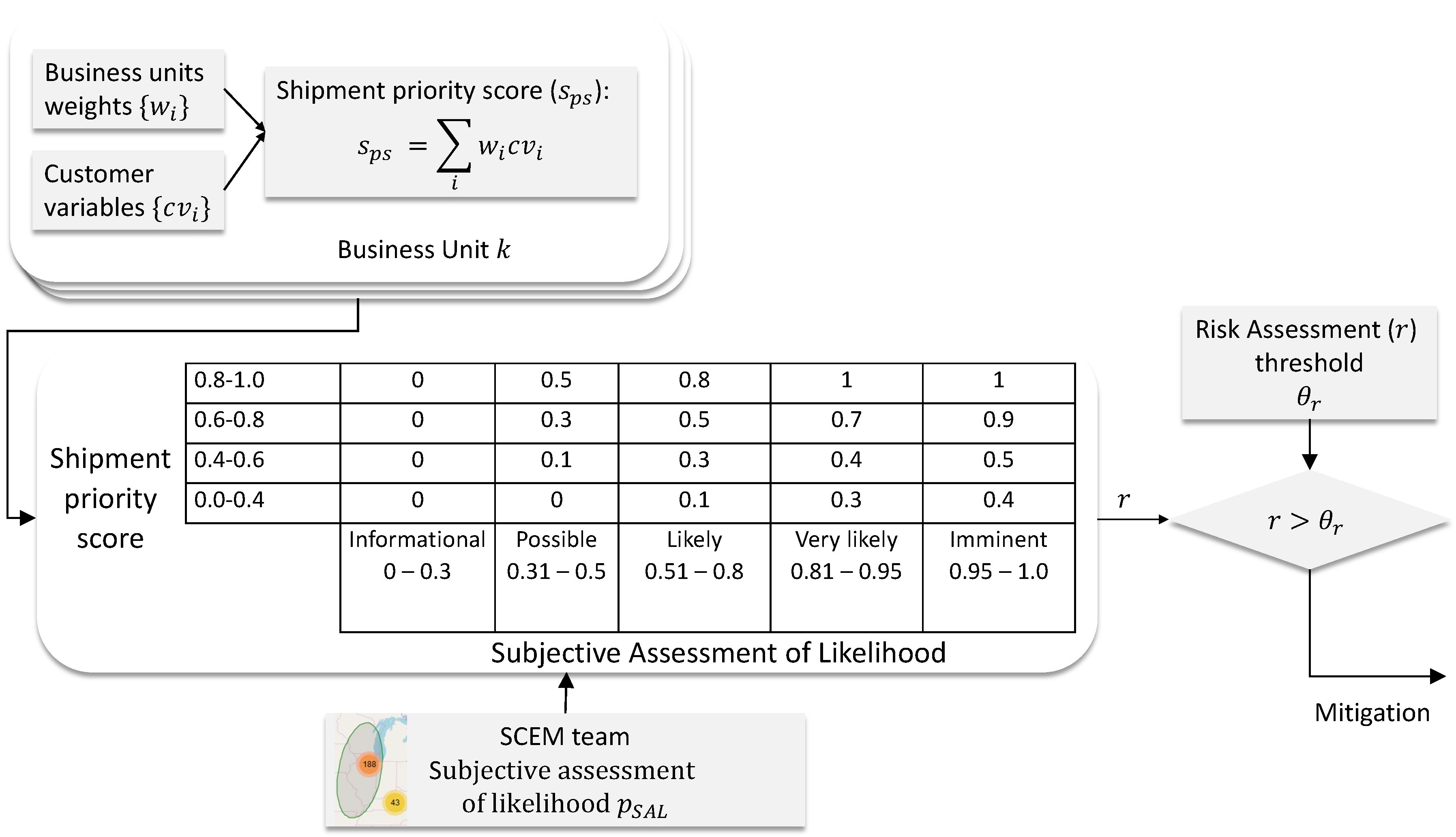
The shipment priority score (SPS) was introduced as a metric that quantifies the importance of a specific shipment. SPS was modeled as a weighted sum of a finite number of n normalized customer variables
where are the associated weights. A customer variable takes values from a finite set of discrete and ordered values, e.g., customer ranking can be modeled as (please note the specific customer variable is fictitious and is here for illustrative purposes only)
The process started with a business unit manager assigning numerical values to the categories, as illustrated in Table 1. Note that the values were subjectively assigned to intuitively capture the relative difference among the categories. In the conceptual example shown in Table 1, the high and very high are relatively close, whereas critical is of considerably higher importance.
To prevent multiple scales associated with different customers from affecting the weights of Equation (1), the customer variables were scaled to 0–1 range before they were used in the sum. The scaling was achieved simply by dividing a numerical value of a customer variable by its maximum possible value for that variable
This normalization provided freedom to a business unit manager when assigning numerical values to the categories of customer variables, allowing them to select whatever scale may be intuitive to them, while keeping the weights unaffected and allowing them to encode only relative importance of different customer variable to the specific business unit.
Within an organization, different business units can customize their customer variables with their numerical values. Business units can employ different weights to express their specific perspective on the relative importance of different customer variables.
2.2. Probability of an Event
In the context of risk assessment and risk management, the probability of an event is typically considered as a subjective assignment, sometimes referred to as a personal probability, in the tradition of [3]; other times as plausibility [4], or belief [5]. In practice, this probability can be obtained directly from an analyst, as a subjective assessment of likelihood (SAL); other times it can be the result of a statistical, computational module. In both cases, the probability estimate of an event is denoted .
The proposed metric SAL is a categorical variable with five intuitive states: informational, possible, likely, very likely, and imminent. A numerical mapping of these variables are summarized in Table 2. As suggested in its name, SAL is a subjective metric. Categories and their associated probability ranges can be adjusted according to the user’s needs and preferences.
3. Geofencing and Risk Assessment
3.1. Event Geofencing and Its Relation to Probability
In the manual mode, an analyst supplied the geofence that defined the region affected by an event, using a flexible shape in the form of a tilted ellipse, characterized by five parameters: latitude and longitude of the center, lengths of the two semi-axes a and b, and the tilt , as illustrated in Figure 1a. While free-form shapes gave an analyst more flexibility in outlining a region of space, they also required more effort. Moreover, simple shapes—fully defined by a few parameters—were easier to modify, track, and store the history of their changes. These features were identified as important to deal with the evolving uncertainties associated with events. Because an ellipse was defined in the longitude–latitude space, it was straightforward to test if a location A defined by its coordinates was inside the geofence
where were the rotated coordinates about the center of the ellipse by the tilt angle
In the simplest implementation, every location within the geofence was assigned the same likelihood , according to Table 2. Using ellipses for geofencing paves the path for refinement of the probabilistic assignment. The same elliptical shape was found useful for modeling both a uniform probability attached to an elliptical geofenced area and for modeling a Gaussian bi-variate probability distribution
where is the covariance matrix
as the vector of the coordinates , is the mean vector of the distribution , and is the Pearson correlation coefficient. This second interpretation of the ellipse, as an equiprobable contour, has the advantage that it avoids abrupt steps in probability, which depicts the natural situation better and is very attractive to higher-level decision makers; however, it also has a disadvantage that it introduces a different way of thinking of probability assignment, which can impede the immediate adoption of the module in practice. Because the intent was to develop an extensible module, we described this interpretation in some detail, but the first implementation, described in Section 4, employed a simple uniform probability interpretation.
When modeling as a probability distribution, the ellipse signified an equiprobable surface, as depicted in Figure 1b. The semi-axis point in the direction of the eigenvalues of the covariance matrix and their length corresponds to the eigenvalues [6]. With this formulation, it was possible to attach smooth, spatially-dependent probabilities over a wider geographic region. In addition, the approach allows for a natural extension for future implementation.
Thus, two different models can be attached to the same user-defined ellipse: a uniform probability or bi-variate Gaussian distribution. The Gaussian model lends itself to additional extensions: one extension can be to employ a mixture model , comprised of weighted Gaussian distributions [7], with k components
where each mixture components (user-defined ellipse) can have separate assessments of likelihood. The coefficients are probabilities in [0, 1] range with and they would have to be computed based on the user inputs when the SAL values associated with individual ellipses are supplied. A conceptual example of a mixture, comprised of three Gaussian is illustrated in Figure 2.
The other direction for extension was to pave the path to Bayesian updating. The need for this updating can arise when the model receives multiple inputs from different users, each providing their own SAL. Conceptually, Bayesian fusion provides consistent and principled inclusion of these [8,9] inputs and provides a mechanism to appropriately weigh the reputation of the users in the form of priors. The concept of conjugate priors, introduced by [10], enables easy updates of the posterior probability distributions in analytic form, avoiding often costly numerical computations. The conjugate prior of a multivariate Gaussian is just Gaussian, but the associate conjugate prior associated with the variance is the inverse Wishart distribution. It is often preferred, that instead of updating the variance, to update its inverse, the precision , with Wishart distribution as the conjugate prior [11]
where the number of degrees of freedom and matrix are parameters of the distribution, with ; tr() signifies the trace of a matrix (the sum of its diagonal components) and is the standard gamma function. It is important to note that specifying the parameters of the Wishart distribution can be challenging. To avoid this complexity, and to facilitate the transition from existing practices, the implementation described in Section 4 did not employ Gaussian distribution and Bayesian updating.
3.2. Risk Assessment
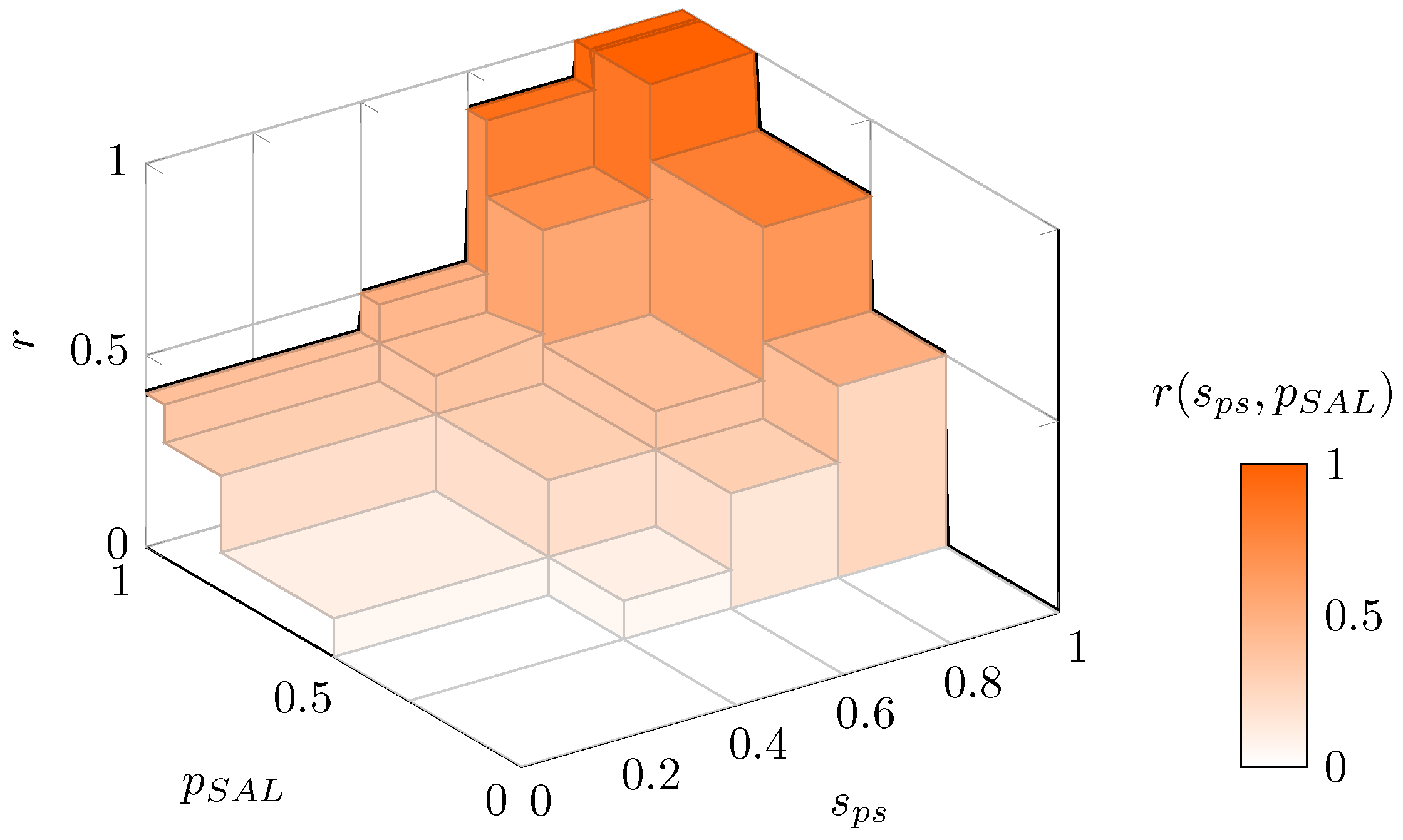
In general, the risk of a decision rule is obtained as an expectation of a loss function [12]. When data are not available, the risk reduces to the loss function. In the proposed framework, risk r is estimated as a nonlinear mapping, where the domain is spanned by the shipment priority score and the subjective assessment of likelihood .
An example mapping, in the form of a look-up table, is defined in Table 3 and illustrated in Figure 3.
Within this specification, the lowest range of SAL corresponded to zero risk, while the lowest range SPS was associated with non-zero risk when SAL was high. As stated above, the specification of Table 3 was based on the user’s preferences; different users may perceive risk differently.
Finally, the estimated risk r is compared to a user-defined, acceptable threshold : shipments with were recommended formitigation, as expressed by the mitigation indicator
The risk computation is summarized in Algorithm 1. The input data consists of the set of all shipments scheduled for the time interval of interest , normalized customer variables with associated weights , geofenced area specified by ellipse parameters (center coordinates , semiaxes a and b, and tilt angle ), SAL , and the risk threshold . The algorithm employs internal normalization for customer variables. After the normalization, it identifies affected shipments that originate or terminate in the geofenced area specified by the ellipse. For each shipment, first calculate the SPS, then risk from the nonlinear mapping, and finally the mitigation indicator function. The output of the algorithm is a set of ordered pairs of mitigation indicators and their associated risks .
| Algorithm 1: Risk calculation. |
 |
4. Implementation
Dow is a very large global manufacturing company that conducts business in more than 160 countries. Dow’s supply chain utilizes a variety of modes of transportation such as: Air, Deep Sea, Inland Waterways, Pipeline, Postal Service, Rail, Road, and Sea [13]. Dow is keenly aware of the ramifications that disruptive events have on its operations, its customers, and its overall profitability. In an effort to advance its existing supply chain event management processes, Dow (and partner organizations) proposed a research project to the Manufacturing x Digital (MxD) Institute (www.mxdusa.org) aimed at improving and further automating the current SCEM process underway at Dow by creating a framework to digitize, integrate, and automate the information pipeline and action workflow, along with offering Dow users recommendations based on prior mitigation actions [13]. The MxD Institute awarded project resulted in the development of five (5) modules that perform independent actions, but when linked together, deliver the desired results applied to outbound Dow shipments. The five modules are as follows:
- Predictive Transit: This module provides an estimated shipment transit time for future shipments based on source, destination, planned shipment date, product type, weather, and event data.
- Risk Assessment: This module provides a graphical user interface (GUI) to enable a user to document current and future events and automatically compute a risk for each individual outbound shipment in the affected geographical area.
- Mitigation Planning: This module automatically sends a communication (text/SMS or email) to subscribed decision makers when an outbound shipment has been promoted by the RA module. The communication provides an overview of the shipment and the event impacting it. The user can then enter in mitigation information, which is stored. After enough mitigation decisions are collected, a machine learning method may be trained to then automate recommended mitigation actions.
- SIMBA Chain Communications: This module integrates relevant data from different modules using a blockchain ledger and sends automated notifications to targeted individuals (Dow internal and external) when risk thresholds are met.
- Performance Analytics: This module is a data enablement SQL table within the Microsoft Azure environment with direct connection to a dashboard that calculates and displays Key Performance Indicators (KPIs) which are derived from the various modules. This module provides aggregated data, along with an easy access point for monitoring and decision making.
Figure 4 depicts interactions among the modules.The focus of this article is the RA module, which received information from users directly (SCEM analysts and business unit managers); read additional information from decision-support data and the predictive transit module; and finally stored the information to Risk Mitigation/Performance database and sent an immutable record to the blockchain. Dow’s expected value from such a system as a result of reductions in disruption incurred freight costs and reductions in disruption related manpower costs is estimated to be 5,000,000 USD over three years in Dow’s Outbound Logistics space for North America [13]. Although the modules described above were developed to be independent, each module was designed with interfaces to pass data to other modules as needed. For example, the RA module can read inputs from the Predictive Transit module, or directly from a human (supply chain event manager). And under the circumstance where the RA module informs the Mitigation Planning module regarding a specific shipment, the RA module and the subsequent modules all coordinate. The implementation of the described methodology for the RA module is depicted in the block diagram of Figure 5.
For all shipments originating or terminating in the event-affected area, SPS , computed from weighted customer variables, and SAL , provided by the SCEM analyst, were mapped through a utility function to produce risk r, which was compared to the acceptable threshold . A shipment with was recommended for mitigation. The RA framework is accessed through a GUI, which connects to the manufacturer’s database and is further described in the Code and Implementation section as well as in the Appendix A. The additional figures in the Appendix A describe how to use the GUI and gives an example of a multi-day geofence. For an event spanning multiple days whose geofences enclose hundreds of shipments, the entire risk assessment computation, including database communication, takes about 20 seconds.
Events with fewer affected shipments complete the risk assessment in less time. In general, an individual shipment’s processing takes a fraction of a second. This includes obtaining geo-location of the shipment, querying associated customer and business unit variables, the entire risk computation, database updates, and GUI updates.
4.1. RA Database Implementation
The database was designed to connect directly to the manufacturer’s shipment data. Data on shipments are queried from the manufacturer’s tables, and the resulting event generation is saved into the RA module’s database, described next. There are several tables in the RA database and they deal with event details, geo-spatial coordinates, risk mapping, business unit weightings, and customer variables. Figure 6 shows the 11 tables used in this implementation.
This implementation featured five customer variables used in determining SPS: Customer_Segmentation_CV, Customer_Contract_Demand_CV, Customer_Distinction_CV, Customer_Rating_CV, and Customer_Margin_CV. Each variable had an associated table with two fields, one for the category or interval that the customer belonged to in that variable, and the other was a value associated with that category or interval, which would be used in normalizing customer variables for the SPS. For example, if the variable was Customer_Segmentation_CV and it contained five levels, each with a name and a relative importance value, then the specific customer associated with the current event’s shipment would have the category and value associated with the variable.
The event tables allowed a user to bring back previous events for updates, or to check on potential changes. If the RA software has been used previously, the first query is sent when the GUI is started, and a table is populated with previous events, from these tables, that the user can select and show on the map. These were events that were previously saved into the events tables. If an SCEM analyst decides to change the settings of a previous event they can choose it here, make the changes, and submit it as an updated event. They are described as follows:
- Events table (top left) contained a unique event ID, date range, event status and category, shipment mode, and some information on whom recorded the event and where, such as event manager, region, updated on, updated number, and finally some user comments if desired.
- Event_Geofence table recorded unique event information, viz. event ID, update number, day in event, as well as the event data and parameters of the geofence: longitude, latitude, A (major axis value), B (minor axis value), and tilt.
- Event_Shipments contained information on the populated shipments from the manufacturer’s database as well as user supplied information for the given event. This table contained four fields that labeled a unique shipment within an event. These were event ID, day in event, shipment ID, and update number. The shipment mode was captured just as it was in the Events table. A column for status was added for tracking in-progress and updated events. SAL and SPS are calculated per shipment per event in order to obtain a mitigation indicator for each shipment, for each event. A comments field was included for user comments, and finally, two additional columns named Human SPS and Human Risk Score were added so a business unit manager could enter their own interpretation of shipment priority and risk to the event.
4.2. Code and Interface
Code was developed using Python [14] in a Jupyter Notebook scientific computational environment [15]. The software used to generate interactive maps in which the SCEM analyst would place geofences and observe shipments was implemented using IPyLeaflet [16], a bridge between Jupyter and the Leaflet [17] mapping library. The module was deployed in Microsoft Azure environment, which served as an integration platform with other modules briefly described above. At the time of the first implementation Jupyter Notebooks in Microsoft Azure could only be set to be either entirely open, or for a single-user. It was not possible to set a notebook to be private and shared by a dedicated team. To overcome this limitation, we deployed the notebooks using Jupyter Hub, which was pre-loaded in Microsoft Azure Ubuntu virtual machine. Then we managed users via the virtual machine. The RA module was contained in a single Python (.py) file and was run by instantiating the module in a Jupyter Notebook. This approach was taken so that the code would not distract the users, and also to protect the code from unintentional modifications. The module contained three classes, which are described in the following section.
The first and simplest class in the module is the database class. It is used to connect and communicate with the manufacturer’s database. It is small and only contains an initialization method for connection, and a simple query method which runs a query and returns all results as an array. There are no parameters to this module. It is called in the initialization method of the event creation class, the second and main class of the module. The event creation class contains all the methods for interacting with the GUI (Figure 7), retrieving and displaying information requested by the analyst, setting off the risk score computation, saving the data to the database, and submitting events to the database, Simba Chain, and mitigation processes.
When the user selects the option to add a geofence to the map, the third class, the geofence class, is used. This class is used to generate an elliptical geofence in the form required for IPyLeaflet to display. The ellipse is made out of 80 points, which are generated from the ellipse equation, which is defined using a center, major and minor axis, and tilt values. These are set by the user when interacting directly with the geofence on the map. Another way the geofence is created is by the selection of a previous event, which uses the stored parameters from past events to generate a geofence for each day in the event and displays them on the map. The RA module was developed in Microsoft Azure and tested using Jupyter Hub [18].
4.3. Users
The four types of stakeholders in the RA module are the SCEM analyst, the system administrator, the business unit manager, and the software developer. The relationship between the module and these four stakeholders is described in turn.
The SCEM analyst would use the interface to manage events: draw the geofence, select type of shipment (road, rail, or both), and assign SAL. The analyst can also update the information related to existing events. They may wish to return to a previous event after new information is learned, and change the GUI values for risk assessment. For example, environmental or social changes may require the geofence locations to be moved. This could relieve certain shipments no longer in the affected area from mitigation and capture new affected shipments that were not part of the original event.
The system administrator sets up the module for additional users, installs software in a new environment and manages permission on the network the RA module is running on, such as database access.
Business unit managers can overwrite the final risk score, or its intermediate results. These are stored in the database and are initially empty rows. The results of the risk score calculation are stored in a table. Additional empty columns have been added for the business unit managers to enter their personal scores by hand. In this module, the two available columns are Human SPS, and overall Human Risk Score. They may wish to return to a previous event after new information is learned, to update the database. These data entries will become increasingly valuable over time as new disruptions in supply chain events lead to different mitigation options. The potential for data-driven learning in future implementations was considered when designing the framework in this way.
Finally, a software developer can reuse, modify, and/or extend the capability of the code.
5. Conclusions
A framework for risk assessment of potentially disruptive events, developed to facilitate a smooth transition from the existing, manual processes towards automation, was introduced. The initial implementation strongly depended on human participation: SCEM analyst provided input probability—SAL, humans also had capability to overwrite the model-estimated relative shipment importance—SPS, and even overall risk. Because the key inputs depended on people, probabilistic models were kept simple, to make the usage more efficient and avoid overwhelming the user.
The framework was illustrated in the Dow case study and implemented in the Jupyter scientific computational environment. MS SQL database tables stored the shipment data, model parameters, event-characterization parameters, and model results. The framework featured the data collection system designed for capturing human decisions that were difficult to articulate, paving the way to the ground truth dataset that will enable future machine learning solutions. In early tests, the initial semi-automated solution suggested great acceleration of the decision making process compared to the traditional manual process, from hours down to seconds.
The framework was designed to be used for outbound shipments in a business-to-business environment. These shipments can include several different types of modes, including air, ship, road, rail (and combinations, i.e., mixed-modes of transport), and can include both domestic and international routes. The intent of the project was to be able to use information that informs the likelihood of an event that could have an impact on outbound shipments, and then develop a decision support platform that allows business personnel to take appropriate actions to mitigate disruption to the manufacturer and/or its customers. Although this use case is fairly broad, the framework can not be applied to all types of transportation problems. Applications where expected transportation time is minutes (e.g., food delivery) would not be a suitable application since it would be unlikely that there would be enough time to determine and implement mitigation actions; however, it does seem likely that the framework could be applied to inbound shipments, as long as accurate data could be obtained regarding planned routes, in transit location, and other relevant data to implement the RA framework. One limitation is that the only uncertainty is related to weather, or similar event; the present framework does not include many other aspects of inbound logistics, such as operations of the suppliers and their dependencies.
Future work will examine the extension to develop additional aspects of inbound logistics. More work is needed in developing the cost models, which will pave the way to more traditional optimization. The next iteration of the implementation will test users’ adoption of the second interpretation of the geo-fence ellipses, as a Gaussian distribution as well as the mixture of Gaussian distributions. Finally, the captured human decisions that disagreed with automated assessments related to SPS, or overall risk, will be used to develop a better data-driven model over time.
Author Contributions
Conceptualization, N.G.N., M.K., and J.A.; methodology, N.G.N. and M.K.; software, N.G.N. and C.J.V.; validation, N.G.N., M.K., and J.A.; formal analysis, N.G.N. and C.J.V.; investigation, M.K., N.G.N., C.J.V., and J.A.; resources, J.A. and P.B.; data curation, J.A.; writing—original draft preparation, N.G.N.; writing—review and editing, M.K., N.G.N., C.J.V., J.A., and P.B.; visualization, N.G.N. and C.J.V.; supervision, M.K., N.G.N., J.A., and P.B.; project administration, M.K., N.G.N., and J.A.; funding acquisition, M.K., N.G.N., and J.A. All authors have read and agreed to the published version of the manuscript.
Funding
This research was funded by MxD Institute grant number 17-02-01.
Acknowledgments
Effort sponsored by the U.S. Government under Agreement number W31P4Q-14-2-0001 between the MXD USA and the Government. The U.S. Government is authorized to reproduce and distribute reprints for Governmental purposes notwithstanding any copyright notation thereon. The views and conclusions contained herein are those of the authors and should not be interpreted as necessarily representing the official policies or endorsements, either expressed or implied, of the U.S. Government. This material is based on research sponsored by Office of the Under Secretary of Defense for Research and Engineering, Strategic Technology Protection and Exploitation, Defense Manufacturing Science and Technology Program under agreement number W31P4Q-14-2-0001. The U.S. Government is authorized to reproduce and distribute reprints for governmental purposes.
Conflicts of Interest
The authors declare no conflict of interest.
Abbreviations
The following abbreviations are used in this manuscript:
| GUI | Graphical user interface |
| RA | Risk assessment |
| SAL | Subjective assessment of likelihood |
| SCM | Supply chain management |
| SCEM | Supply chain and event management |
| SCRM | Supply chain risk management |
| SPS | Shipment priority score |
Nomenclature
| A customer weight | |
| Geofence longitude coordinate | |
| Geofence latitude coordinate | |
| a | Geofence major axis |
| b | Geofence minor axis |
| Geofence tilt angle | |
| Gaussian mean | |
| Gaussian covariance | |
| Gaussian variance component to | |
| Gaussian mixture coefficients | |
| Pearson correlation coefficient | |
| Mitigation indicator | |
| Subjective assessment of likelihood probability | |
| Gaussian mixture components | |
| Wishart distribution | |
| Precision matrix, the inverse of the covariance matrix | |
| Set of all shipments on within the specified time interval | |
| Set of affected shipments | |
| V | Wishart parameter matrix |
| Gamma distribution, | |
| L | Loss function for mapping risk (implemented as a look-up table) |
| Customer variable category | |
| Customer variable value | |
| Customer variable normalized value | |
| r | Risk |
| Risk threshold | |
| Shipment priority score |
Appendix A. Implementation Details
The appendix provides some implementation details. Figure A1 shows the graphical user interface in operation, with annotations associated with different user interactions.
The multi-day geofence is created by selecting the start and end days from the date selection widget in the interface (Figure A2).
Once the event start and end dates are selected the Event Days list is populated. The creation of a three day event is shown below in Figure A3 which shows associated SAL values for each day, and Figure A4 which shows the geofence for each day. The geofence locations were selected to simulate a weather-disruption pattern with growing uncertainty over the three days.
Figure A1.
Full graphical user interface (GUI) quick-reference guide.

Figure A2.
Selecting event start and end dates in the interface.

Figure A3.
Setting subjective assessment of likelihood (SAL) values for a three-day geofence.

Figure A4.
An example of a multi-day geofence.

References
- Vishnu, C.; Sridharan, R.; Kumar, P.R. Supply chain risk management: Models and methods. Int. J. Manag. Decis. Mak. 2019, 18, 31–75. [Google Scholar]
- Bearzotti, L.A.; Salomone, E.; Chiotti, O.J. An autonomous multi-agent approach to supply chain event management. Int. J. Prod. Econ. 2012, 135, 468–478. [Google Scholar] [CrossRef]
- Savage, L.J. The Foundations of Statistics; Dover Publications, Inc.: Garden City, NY, USA, 1972. [Google Scholar]
- Jaynes, E.T. Probability Theory: The Logic of Science; Cambridge University Press: Cambridge, UK, 2003. [Google Scholar]
- Theodoridis, S. Bayesian learning: Inference and the EM algorithm. In Machine Learning: A Bayesian and Optimization Perspective; Academic Press: Cambridge, MA, USA, 2015; Chapter 12; p. 586. [Google Scholar]
- Duda, R.O.; Hart, P.E.; Stork, D.G. Bayesian decision theory. In Pattern Classification, 2nd ed.; Wiley-Interscience, John Willey & Sons Inc.: Hoboken, NJ, USA, 2001; Chapter 2; pp. 33–36. [Google Scholar]
- Bishop, C.M. Mixture of gaussians. In Pattern Recognition and Machine Learning; Springer: Berlin/Heidelberg, Germany, 2006; Chapter 2; pp. 110–113. [Google Scholar]
- Pearl, J. Probabilistic Reasoning in Intelligent Systems: Networks of Plausible Inference; Morgan Kaufmann: San Francisco, CA, USA, 1988. [Google Scholar]
- Koller, D.; Friedman, N. Probabilistic Graphical Models: Principles and Techniques; MIT Press: Cambridge, MA, USA, 2009. [Google Scholar]
- Raiffa, H.; Schlaifer, R. Applied Statistical Decision Theory; Division of Research, Graduate School of Business Administration: Harvard, MA, USA, 1961. [Google Scholar]
- Bishop, C.M. Exponential family. In Pattern Recognition and Machine Learning; Springer: Berlin/Heidelberg, Germany, 2006; Chapter 2; pp. 113–117. [Google Scholar]
- Berger, J.O. Utility and loss. In Statistical Decision Theory and Bayesian Analysis, 2nd ed.; Springer: Berlin/Heidelberg, Germany, 1985; Chapter 2; pp. 46–73. [Google Scholar]
- Archbold, J. Supply Chain Risk Alert; Technical Report 17-02-01; MxD Institute: Chicago, IL, USA, 2019. [Google Scholar]
- Van Rossum, G.; Drake, F.L., Jr. Python Tutorial; Centrum voor Wiskunde en Informatica Amsterdam: Amsterdam, The Netherlands, 1995. [Google Scholar]
- Kluyver, T.; Ragan-Kelley, B.; Pérez, F.; Granger, B.; Bussonnier, M.; Frederic, J.; Kelley, K.; Hamrick, J.; Grout, J.; Corlay, S.; et al. Jupyter notebooks—A publishing format for reproducible computational workflows. In Positioning and Power in Academic Publishing: Players, Agents and Agendas; Loizides, F., Schmidt, B., Eds.; IOS Press: Amsterdam, The Netherlands, 2016; pp. 87–90. [Google Scholar]
- Mease, J. Bringing ipywidgets Support to plotly. py. In Proceedings of the 17th Python in Science Conference (SciPy 2018), Austin, TX, USA, 9–15 July 2018; Available online: http://conference.scipy.org/proceedings/scipy2018/ (accessed on 15 May 2020).
- Derrough, J. Instant Interactive Map Designs with Leaflet JavaScript Library How-to; Packt Publishing Ltd.: Birmingham, UK, 2013. [Google Scholar]
- Jupyter-Team. Jupyterhub Documentation. Available online: https://jupyterhub.readthedocs.io/en/stable/ (accessed on 30 September 2019).
Figure 1.
(a) Tilted ellipse in the longitude–latitude (-) space. (b) Probability distribution assigned to a geofenced area, with an elliptical geofence as the line of equal probability.
Figure 1.
(a) Tilted ellipse in the longitude–latitude (-) space. (b) Probability distribution assigned to a geofenced area, with an elliptical geofence as the line of equal probability.

Figure 2.
A mixture mode with three weighted Gaussian components.

Figure 3.
Risk r as a function of the shipment priority score and assessment of likelihood , as defined in Table 3.
Figure 3.
Risk r as a function of the shipment priority score and assessment of likelihood , as defined in Table 3.

Figure 4.
Relationships among the modules (adapted from [13]).
Figure 4.
Relationships among the modules (adapted from [13]).

Figure 5.
Risk assessment (RA) block diagram.

Figure 6.
The 11 tables used in the RA database.

Figure 7.
A graphical user interface for drawing geofences, observing affected shipments, and submitting events to the RA module.
Figure 7.
A graphical user interface for drawing geofences, observing affected shipments, and submitting events to the RA module.


Table 1.
An example mapping between categories and their associated numerical values.
| Category | Numerical Value | Normalized Value |
|---|---|---|
| high | 3 | 0.375 |
| very high | 4 | 0.500 |
| critical | 8 | 1.000 |
Table 2.
Subjective assessment of likelihood.
| Category | Probability Range |
|---|---|
| Imminent | 0.95–1.00 |
| Very likely | 0.80–0.95 |
| Likely | 0.50–0.80 |
| Possible | 0.30–0.50 |
| Informational | 0.00–0.30 |
Table 3.
Risk assessment table .
| Subjective Assessment of Likelihood | ||||||
|---|---|---|---|---|---|---|
| Informational | Possible | Likely | Very Likely | Imminent | ||
| 0–0.3 | 0.3–0.5 | 0.5–0.8 | 0.8–0.95 | 0.95–1.0 | ||
| SPS | 0.8−1.0 | 0 | 0.5 | 0.8 | 1 | 1 |
| 0.6−0.8 | 0 | 0.3 | 0.5 | 0.7 | 0.9 | |
| 0.4−0.6 | 0 | 0.1 | 0.3 | 0.4 | 0.5 | |
| 0.0−0.4 | 0 | 0.0 | 0.1 | 0.3 | 0.4 | |
© 2020 by the authors. Licensee MDPI, Basel, Switzerland. This article is an open access article distributed under the terms and conditions of the Creative Commons Attribution (CC BY) license (http://creativecommons.org/licenses/by/4.0/).
Share and Cite
MDPI and ACS Style
Krystofik, M.; Valant, C.J.; Archbold, J.; Bruessow, P.; Nenadic, N.G. Risk Assessment Framework for Outbound Supply-Chain Management. Information 2020, 11, 417. https://0-doi-org.brum.beds.ac.uk/10.3390/info11090417
AMA Style
Krystofik M, Valant CJ, Archbold J, Bruessow P, Nenadic NG. Risk Assessment Framework for Outbound Supply-Chain Management. Information. 2020; 11(9):417. https://0-doi-org.brum.beds.ac.uk/10.3390/info11090417
Chicago/Turabian StyleKrystofik, Mark, Christopher J. Valant, Jeremy Archbold, Preston Bruessow, and Nenad G. Nenadic. 2020. "Risk Assessment Framework for Outbound Supply-Chain Management" Information 11, no. 9: 417. https://0-doi-org.brum.beds.ac.uk/10.3390/info11090417
Note that from the first issue of 2016, this journal uses article numbers instead of page numbers. See further details here.