Private Car O-D Flow Estimation Based on Automated Vehicle Monitoring Data: Theoretical Issues and Empirical Evidence

Abstract

Data on the daily activity of private cars form the basis of many studies in the field of transportation engineering. In the past, in order to obtain such data, a large number of collection techniques based on travel diaries and driver interviews were used. Telematics applied to vehicles and to a broad range of economic activities has opened up new opportunities for transportation engineers, allowing a significant increase in the volume and detail level of data collected. One of the options for obtaining information on the daily activity of private cars now consists of processing data from automated vehicle monitoring (AVM). Therefore, in this context, and in order to explore the opportunity offered by telematics, this paper presents a methodology for obtaining origin–destination flows through basic info extracted from AVM/floating car data (FCD). Then, the benefits of such a procedure are evaluated through its implementation in a real test case, i.e., the Veneto region in northern Italy where full-day AVM/FCD data were available with about 30,000 vehicles surveyed and more than 388,000 trips identified. Then, the goodness of the proposed methodology for O-D flow estimation is validated through assignment to the road network and comparison with traffic count data. Taking into account aspects of vehicle-sampling observations, this paper also points out issues related to sample representativeness, both in terms of daily activities and spatial coverage. A preliminary descriptive analysis of the O-D flows was carried out, and the analysis of the revealed trip patterns is presented.

1. Introduction

To date, transportation engineering has focused on models and methods for obtaining travel demand flows as well as investigating travel behaviour [1,2,3,4,5,6,7,8]. Indeed, demand plays a key role in analysing and modelling transportation systems, since transportation projects are motivated by the need to satisfy transportation demand. In turn, traveller choices can significantly affect the performance of supply elements through congestion. Therefore, due to the need to obtain reliable origin–destination (O-D) demand flows, much of the literature has dealt with origin–destination (O-D) flow estimation and forecasting [8,9,10,11,12,13,14,15,16,17,18,19].

Typically, to estimate current demand flows, surveys can be carried out, usually by interviewing a sample of users (direct estimation), and demand can be derived using results from sampling theory. Estimation of current origin–destination demand flows can be improved by combining the estimators with aggregate information related to O-D demand flows [20]; e.g., traffic counts: counts of user flows on some elements—links—of the transportation supply system—transportation network). Alternatively, demand (present and future) can be obtained by modelling systems. While the former provides actual/current matrices with which, when assigned to the network, flows closest to traffic counts are reproduced, the latter allows O-D flows to be linked with land use, socio-economic factors, and level-of-service attributes. Therefore, the effects due to changes occurring in future scenarios on such factors can be assessed.

As summarised below, O-D flow estimation using traffic counts is the focus of great interest due to the amount of data coming from the transportation network [21]. Indeed, there are currently issues capturing door-to-door travel characteristics using traditional methods. Avenues of progress are being opened up by the development of new technologies to automate and facilitate disaggregate data collection, such as GPS devices, cellular-network positioning from call and activity data and smartphone sensors, point-to-point detection sensors [22], licence plate recognition [23], bluetooth [24], and radio-frequency identification [25]. The opportunity offered by telematics and the penetration of tracing/tracking services on car movements (i.e., floating car data—FCD), which allow continuous information in time and space to be obtained, gave rise to the prime objective of this paper: to investigate urban private transport through automated vehicle monitoring (AVM/FCD) data in order to identify trip characteristics and infer origin–destination demand flows from cars (private vehicles).

The development of telematics during the last 30 years has significantly enhanced research possibilities in the field of transportation, also impacting on traditional survey methods. Classical survey methods for collecting travel data have been adapted to the digital era. For instance, travel diary-based approaches have been transformed into electronic travel diaries with global positioning systems (GPS), thereby speeding up data transfer from users to research groups and providing details for understanding more in-depth travel patterns [26,27,28,29,30]. Innovation has also driven transport system modelling: reverse assignment procedures have been developed to update network and demand model parameters [11,18]; In particular, in transit modelling, smart-card data were used to estimate the origin–destination matrix as well as calibrate and validate assignment models ([17,31,32,33,34,35].

By the same token, freight demand modelling benefits from telematics, especially in revealing empirical [36,37,38,39] and in modelling delivery tours [40,41,42,43,44]. Of course, the challenge is to obtain data from private freight operators to measure and evaluate the market. This is non-trivial, given that operators avoid sharing data, as they are aware that they risk losing competitive advantage given that such technology is usually used for supporting fleet management and insurance issues [42,45,46]; The collected data can be used to refer only to vehicle location tracked second by second, allowing spatial and timeframe features of the tours made to be assessed.

While automated vehicle monitoring (AVM) data (including GPS) for vehicles are increasingly available due to the deployment of telematics in vehicles with the aim of providing further services [47], as well as for insurance purposes, methods to process such data with the objective of analysing and modelling trip chains (i.e., sequence of daily trips for performing daily activities) have not been fully explored with regard to the implication of underlying origin–destination demand flows by car.

To investigate origin–destination flows, the travel patterns followed by private vehicles (cars) have to be identified, as summarised in Section 2. Trip chains are an important element of vehicle movements in an urban or metropolitan setting for estimating origin–destination flows that, once assigned to the network, allow link flows to be obtained and traffic impact to be estimated. Thus, as stated above, the main objective of the paper is to study the chief characteristics of private vehicles (cars), identifying their trip patterns and their daily activity, as well as using the information collected to estimate an origin–destination matrix to be used for analysing transport systems. In particular, the sample O-D matrix is extracted from AVM/FCD data, and subsequently, their representativeness is evaluated, as discussed in Section 4. In fact, devices from which transportation data can be obtained concern a portion of a population whose representativeness is not always easily available to researchers/technicians (e.g., private cars equipped with on-board units to reduce insurance costs [48]. Secondly, the statistical significance of the estimates obtained [49,50,51,52], as well as goodness in reproducing vehicle link flows, should be pointed out. Thus, the opportunity offered by AVM data is explored. The data source consisted of a sample of about 30,000 cars (388,000 trips) travelling on five working days within the Veneto region (Northern Italy) in October–November 2018.

The paper is organised as follows. Section 2 outlines the literature on the usage of AVM/FCD for route analysis and simulation as well as on O-D estimation, while Section 3 presents the methodology and its implementation to a real test case. Section 4 summarises our results, and some conclusions and further developments are discussed in Section 5.

2. Literature Review on FCD Usage

An emerging research challenge is to use FCD to describe users’ mobility behaviour as well as route choices. Therefore, the literature on the use of FCD for simulating route choice is reviewed below, which is followed by examination of the procedures developed for origin–destination demand flows.

2.1. Path Choice and Route Attribute Evaluation

In general, AVM/FCD contain three different levels of data: basic information about vehicle ID, location, time attributes and driving direction, vehicle information, which includes a vehicle’s status data (gear, brakes, etc.), and extended information that provides video frames [53]. To assess the travel demand patterns, the first-level data, i.e., basic information, are commonly used. This dataset is collected based on GPS systems, which allow definition of the space–time features of the trips undertaken. Following the same lines, Ehmke et al. [54], Rahmani et al. [55,56], and Tu et al. [57] studied the time attributes of trips using FCD. Tu et al. [57] proposed a new approach to investigate the time-varying shortest path. The approach assumes reconstruction of the traffic conditions from discrete space–time points to traffic flows by using a map-matching procedure. This allows the paths used by vehicles to be tracked, together with their speeds. More than 11,000 taxi-based floating car data in Wuhan (China) showed that the shortest paths of the same O-D pair change with the spatio-temporal varying traffic state.

Ehmke et al. [54] showed that FCD can be a very useful source for describing time-dependent travel times in a network. They used FCD from a taxi service in Stuttgart (Germany) and identified 100 O-D pairs. Different levels of aggregation in determining time-dependent travel times from a database of historical FCD are presented and evaluated with regard to routing quality.

Rahmani et al. [55] developed a non-parametric method to estimate route travel time distribution using low-frequency floating car data. Considering the problem of low polling frequency for FCD, Rahmani et al. [55] proposed a new method for reconstructing the vehicles’ travelled paths and merging them into the entire routes. Subsequently, given that estimation of urban network link travel times from sparse FCD usually needs pre-processing, mainly map-matching and path inference for finding the most likely vehicle paths are dealt jointly; in fact, paths have to be consistent with reported locations. Path inference requires a priori assumptions about link travel times that can be unrealistic and affected by bias with issues in shortest path identification. Therefore, Rahmani et al. [56] developed a combined procedure for path inference and travel time estimation using FCD from taxis in Stockholm (Sweden).

Dewulf et al. [58] studied FCD-based trips made by 400,000 vehicles between 6651 traffic zones of Flanders (Belgium). They traced the travel times for every monitored vehicle, which were used to obtain the aggregated model on generic travel time for peak and off-peak periods for the complete road network of the case study. Thus, using FCD, they revealed the commuting patterns for inter-city and intra-city trips and detected the congested directions of the study area, thereby contributing to more precise prediction of travel times compared with free flow-based models.

Yamamoto et al. [59] and Cao et al. [60] estimated link flows using observed link speeds from FCD, while Croce et al. [61] focused on the use of FCD to define perceived alternative paths (choice set) and the choice of one path in the path choice set. Stipancic et al. [62] examined vehicle manoeuvres using GPS data from smartphones of vehicle drivers and explored their potential as surrogate safety manoeuvres through correlation with historical collision frequency and severity across different facility types.

2.2. O-D Demand Flow Estimation

FCD are also considered as the basis for estimating O-D matrices [16,39,58,63,64,65,66,67,68]. Carrese et al. [64] proposed the dynamic estimation O-D matrix approach using FCD. Based on a district road network in Rome, they monitored 12 O-D flows with FCD to assess route choice probabilities and compare them with travel demand generated for 38,000 vehicles in one hour. The results show the great potential of FCD for the dynamic demand estimation problem, allowing enhancements in the accuracy of O-D travel times and route choice probability reproduction. Moreover, the authors revealed the greater importance of FCD than information received from traffic counts, although they used a limited number of monitored vehicles and a small study area (only 54 traffic zones and 400 regular nodes).

Another step to justify the benefits of FCD usage was made by Yang et al. [65], who developed the O-D flow model based on sampled GPS positions of probe vehicles. Considering the map matching procedure, they described the sampled O-D flows and, using the generalized least square method, defined the actual travel demand. The traffic count data were taken as the basis for O-D demand updating. Sbaï et al. [66] proved the necessity of data fusion from several tele sources such as FCD (taxis with GPS detectors), loop detectors, and smartphones. Among the tele sources studied, Sbaï et al. [66] estimated FCD as being more reliable for travel demand assessment but noted the problem of a small share of taxis in the total traffic. This resulted in difficulties for data extrapolation to the whole population. Sbaï et al. [66] also revealed the differences in taxi drivers’ behaviour from that of regular car drivers, such as higher travel speed and more frequent stops to enable passengers to board or alight.

Guo et al. [69] focused on estimation of origin–destination trips and proposed an approach to the discovery and understanding the spatio-temporal patterns of movements. They used a large dataset from Shenzhen (China) to test and validate the proposed methodology. Tang et al. [70] focused on taxi trips extracted from GPS data. Then, the travel distance, time, and average speed in occupied and non-occupied status are used to investigate human mobility. They estimated the OD matrix of the inner area of Harbin city and modelled the traffic distribution patterns based on the entropy-maximizing method. Nuzzolo et al. [39] used sampled FCD on 310 taxis in Rome to assess the list of the space–time attributes, revealing the behaviour of taxi trips. Among the main findings of the study, the authors identified demand peaks on Monday morning and Saturday night as well as a very small number of requests for service on Sunday. Analysis of the spatial features of the trips made revealed high-density O-D flow distribution within the Inner Railway Circle (i.e., city centre) and that Fiumicino airport was a huge attractor. The distribution of trip distance showed the prevalence of O-D flows undertaken in the interval from 2 to 5 km. Thus, the basic space–time features of the taxi service in Rome were identified, and the benefits of using autonomous vehicle services to provide an on-demand service in the future were investigated.

Vogt et al. [67] and Dabbas et al. [68] implemented the O-D matrix calculation according to a double-constrained gravity model with FCD usage for impedance function formalization. Tracking the single vehicle trajectories and defining the number of turns made according to FCD allowed Vogt et al. [67] and Dabbas et al. [68] to form the values of the impedance function for every O-D pair in the matrix. Thus, by tracking the route choice along with zone capacity estimation based on FCD, the authors of both studies implemented the O-D flows calculation. The data were calibrated with information obtained from traffic counts according to an information minimization model. The results presented in both studies indicate the increase in computation accuracy if FCD are used for travel demand assessment. Finally, Mitra et al. [16] developed a methodology for obtaining demand matrices without any prior information but starting from FCD including info on vehicle trajectories. The procedure was successfully tested in Turin (Italy).

In summarise, it may be concluded that FCD/AVM have been successfully used both for monitoring paths used by each vehicle and for obtaining link flows (microscopic level) as well as for large-scale simulation of transportation systems (e.g., macroscopic level). However, further research efforts are required to go beyond such preliminary results, especially to obtain timely O-D demand flows. Therefore, a methodology for obtaining present O-D demand flows by car is presented below.

3. Methodology

To identify private vehicle (car) O-D matrices from AVM/FCD samples, a procedure was developed and tested. Its main feature is that it only uses raw GPS data to detect user activity stops, thus estimating the speed, distance travelled, and status of the engine. Such data, as discussed in Section 2, are anonymised for avoiding privacy issues and have been used for investigating travel patterns; however, a few studies pointed out the opportunity to identify trips and subsequently for O-D estimation. Then, it emerges that further work is needed for investigating technical challenges as well as theoretical issues related to sampling.

The proposed methodology consists of three main steps depicted in Figure 1: car trip detection, sample O-D matrix, and O-D matrix. The first two steps are preparatory to the last, which, instead, represents the focus of this research. Therefore, a description of each step is given below.

Consider a region divided into a set of zones in which the monitored vehicles drive. Once the study area is identified and zoning is performed, for each survey day, the procedure for the daily O-D demand flow estimation consists of the following steps (Figure 1):

• Car trip detection: according to some predefined rules, this stage aims to detect the activity stops performed by each sampled vehicle; therefore, the individual trips (with origin and destination) undertaken by each surveyed vehicle can be obtained;
• Sample O-D matrices; according to study area zoning, the origin and destination of each sample vehicle trip is identified; then, through an aggregation procedure, the sampled O-D vehicle trips are then merged in order to obtain the daily (or timely) O-D matrix;
• Expansion to the universe of investigation; in this step, the sample daily (or timely) O-D matrices need to be expanded to the universe of observation in order to obtain the daily/timely-dependent vehicle O-D matrices of the study area. This step can be considered the core of the procedure, given that the statistical significance of the sample needs to be determined.

3.1. Car Trip Detection

According to the purpose of the procedure developed (i.e., estimation of the O-D matrices from AVM/FCD), and given that such O-D matrices represent the spatial characterisation of trips made by grouping them by place (zone or centroid) of origin and destination, the first stage is to identify such places of origin and destination. In this context, a trip is defined as the act of moving from one place (origin) to another (destination) in order to carry out one or more activities.

Let $\left(ID,t,s,\langle x,y\rangle \right)$ be the probe (monitored/surveyed) vehicle datum. It allows vehicle location and status to be identified. ID is the vehicle identification code, t is the time when the datum is obtained, s is the status of the vehicle engine, and $\langle x,y\rangle$ are the GPS coordinates, i.e., latitude and longitude. With two consecutive data of a given vehicle, the significant changes in vehicle position (i.e., $\langle x,y\rangle$) according to relevant status s can be detected, and then, the origin and destination of a trip can be identified. A sequence of trips, following each other in such a way that the destination of one trip coincides with the origin of the next, is referred to as a journey or trip chain [17]. Therefore, from the fine-grained AVM/FCD, the activity stops need to be identified.

The procedure proposed in this paper is based on the speed and engine status of a vehicle measured minute by minute. The procedure, shown in Figure 1, evaluates these measures so as to determine whether the vehicle has completely stopped or is moving at a very slow speed. The most significant source of errors in classifying stopping events from vehicle data are observations wherein the vehicle has stopped at a bottleneck, but when evaluating its speed, it appears parked. By evaluating both speed during the previous time interval, as well as the GPS data and engine status, the procedure ensures that only activity stops (e.g., longer than a pre-fixed threshold and far from while-travel intermediate/service sites, such as petrol stations) are classified as such in the result.

3.2. Sample O-D Matrices

Once the trips belonging to a trip chain have been identified, the next step is the spatial characterization of trips made by grouping them by place (transport zone) of origin and destination. This information (demand flows) can be arranged in tables as O-D matrices, whose rows and columns correspond to the different origin and destination zones, respectively. Then, we can discretize every transport zone as the array of the following coordinates:

$${{\rm Z}}_i=\left\{{\langle \phi ,\lambda \rangle }_j\right\}$$

(1)

where Z_i is a transport zone i presented as the array of coordinates ${\langle \phi ,\lambda \rangle }_j$ relative to a generic point j spatially within the zone border.

Hence, having obtained the vehicle datum $\left(ID,t,s,{\langle \phi ,\lambda \rangle }_j\right)$, classified as origin or destination of a trip according to an earlier step, the location ${\langle \phi ,\lambda \rangle }_j$ is evaluated in order to identify the relative traffic zone. This means that ${\langle \phi ,\lambda \rangle }_j$ belongs to Z_a only if

$${\langle \phi ,\lambda \rangle }_j\in Z_a.$$

Accordingly, zone Z_j can be grouped into larger administrative units, such as municipalities and provinces:

$${\Omega }_p=\left\{Z_j\right\}$$

(2)

where ${\Omega }_p$ is the total set of transport zones within the administrative district p.

Subsequently, the number of trips from origin zone o to destination zone d can be obtained as follows:

$$V{C}_{od}={\displaystyle \sum _j{T}_{j,od}^{}}$$

(3)

where T_j,od is the generic trip j revealed with origin zone o (Z_o) and destination zone d (Z_d).

The O-D matrix obtained can be characterised for time slice h (selecting only trips belonging to a given time slice h), vehicle type (selecting only trips belonging undertaken by a given vehicle type), and so on.

3.3. Expansion to the Universe of Investigation

Once the sample O-D matrices for different survey days or times are determined, current travel demand can be estimated starting from these results. Then, knowledge of sampling units (vehicles) and the method for enumerating the population universe (e.g., lists of registered vehicles in a traffic zone or counts of passing vehicles) are required. This represents one of the main issues in adopting such FCD/AVM data for travel demand forecasting. Indeed, the issue of estimating O-D demand flows depends on the sampling strategies used, and it is also important to investigate sample representativeness both in terms of trip production and attraction.

Assume that the total statistical population (vehicles) is divided into K classes (e.g., vehicles registered in a province) or strata. Let k be the generic stratum with a population of N_k vehicles: n_k elements are drawn from each stratum.

If $T_{od}^{ik}$ is the number of trips with the required characteristics (e.g., starting in the morning) undertaken by the i-th element (vehicle) in the sample of stratum k, an estimate of the total number of trips can be obtained as follows [20]:

$$\widehat{V}{C}_{od}=N\cdot {\displaystyle \sum _k{w}_k}\cdot {\displaystyle \sum _i{T}_{od}^{ik}/n_k}=N\cdot {\displaystyle \sum _k{w}_k}\cdot {\overline{T}}_{od}^k$$

(4)

where ${\overline{T}}_{od}^k$ is the average number of trips observed in the k-th stratum, and w_k is the weight of stratum k with respect to the universe N.

According to Cascetta [17], the variance of the stratified sampling estimate, $\widehat{V}{C}_{od}$, can be estimated as follows:

$$Var\left[\widehat{V}{C}_{od}\right]\approx N^2\cdot {\displaystyle \sum _k{w}_k^2}\cdot {\widehat{s}}_k^2\cdot \left(1-{\alpha }_k\right)/n_k$$

(5)

where

• ${\widehat{s}}_k^2$ is the sample estimate of the variance of the variable $n_{od}^{ik}$:

  $${\widehat{s}}_k^2=1/\left(n_k-1\right)\cdot {{\displaystyle \sum _i\left(T_{od}^{ik}-{\overline{T}}_{od}^k\right)}}^2.$$
• α_k is the sampling rate in the k-th stratum.

Such issues are discussed below, and empirical evidence is shown to verify the goodness of O-D demand flow estimation using FCD/AVM data.

4. Application to a Real Test Case

This section reports the application of the methodology used to estimate O-D demand flows in the Veneto region (northern Italy). The application was carried out to ascertain to what extent the objective of using FCD/AVM data to estimate transportation demand flows might be realistic. Our investigation was performed by analysing a large dataset of private cars driving in the region. The results allowed trip-chaining patterns to be identified and helped reconstruct O-D trip flows as well as road link flows.

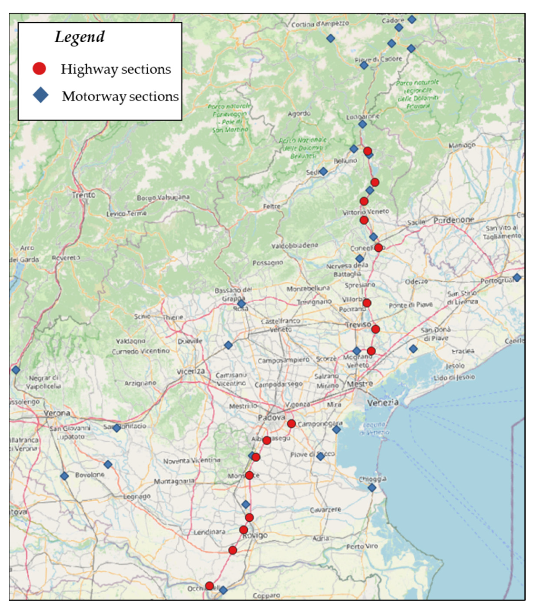
4.1. The Study Area and Available Data

The study area is the Veneto region with its seven provinces. It has an area of 18,391 km² and 4,905,037 inhabitants. The main socio-economic characteristics of the region are summarised in

Table 1. Statistical data for the Veneto region.

Province	Area, [km2]	Inhabitants	Males	Females	Number of Cars	Average No. of Vehicles per Inhabitant	Sampled Vehicles *
Belluno	3678	204,900	49%	51%	135,261	0.660	918 (0.7%)
Padua	2141	936,740	49%	51%	603,290	0.644	7503 (1.2%)
Rovigo	1789	236,400	49%	51%	159,231	0.674	420 (0.3%)
Treviso	2477	887,420	49%	51%	588,052	0.663	5875 (1.0%)
Venice	2463	853,552	48%	52%	471,324	0.552	3274 (0.7%)
Verona	3121	922,821	49%	51%	614,838	0.666	3870 (0.6%)
Vicenza	2722	863,204	49%	51%	577,339	0.669	7298 (1.3%)
Total	18,391	4,905,037	49%	51%	3,149,335	0.642	29,158 (0.9%)

* sample rate in brackets.

(sources: ISTAT [71], ACI [72]).

The provinces of the Veneto region are roughly equivalent in population terms, except for Belluno and Rovigo, which have approximately four times fewer inhabitants. These provinces also have the smallest number of registered cars in the region. Estimation of car motorization level allowed identification of the variation of this parameter by province within a range from 552 to 673 cars per 1000 inhabitants. As shown in Table 1, the number of cars per inhabitant is quite similar in the whole region, except in Venice where it is about 14% less than the average regional number.

4.2. Car Trip Detection

Mobility by car within the Veneto region was investigated through FCD/AVM data, which according to some criteria, such as its large volume and by-product nature, can be considered big data. The collected data consist of information related to car trips within the Veneto region (i.e., at least one survey datum inside the region on the survey day) from the first to the last trip performed in the whole day. The data were analysed to identify travel patterns, thereby obtaining indications on the trips performed. The available database consists of five working-day observations, spread over the autumn months (i.e., October–November 2018) in different working days. For each sampled vehicle, the information form contains the basic vehicle data such as vehicle class, brand, year, type, fuel type and gross weight. The daily car operation logs contain all trips made by the surveyed vehicle in chronological order: vehicle identifier, date (date the record is logged), timestamp (time the record is logged), coordinates (geographical location: latitude and longitude), instantaneous speed, type of road (urban, extra-urban, freeway), and direction angle. No information on the type of activity carried out or the registered trip purpose of surveyed vehicles (e.g., work or university) was available. After extensive cleaning and elimination of observations with missing data, the remaining data were processed in order to investigate travel patterns and trips undertaken. In all, 29,158 vehicles were analysed, corresponding to about 70,000 trip chains undertaken in five days.

Subsequently, the daily vehicle operation logs were analysed in order to identify trips, as introduced in Section 3. Empirical rules (e.g., stopping longer than 20 min far from a petrol station) were used to determine whether the trip reached its destination to perform an activity. It allowed trip origin and destination to be identified and the dataset as pictured in Figure 2 was built.

The dataset “vehicles” reports information about private cars for each observation day and allows the sampling rating to be obtained. The primary key vehicle identification number allows vehicles to be combined with daily trips performed and stored in a dataset “trip description”. This dataset stores the whole information on every trip undertaken on the basis of origin and destination coordinates. It represents the input for the second stage of the procedure described in Section 3 above for the definition of the sampling O-D matrix. Finally, in the dataset “trip details”, the detailed information on the intermediate GPS data from trip origin towards trip destination is reported. This dataset allows us to track the trip chains made by every sampled vehicle through km-by-km or minute-by-minute information.

As stated above, our dataset refers to data from private vehicles (cars) driving at least along one road link of the Veneto region during one of the days in question. In particular, data covering different working days provided the opportunity to point out daily variations in terms of number of trips performed as well as origin–destination (spatial) coverage: 15.10 (Monday), 22.10 (Monday), 7.11 (Wednesday), 15.11 (Thursday), and 23.11 (Friday). It should be noted that the surveyed vehicle was studied for twenty-four hours with the possibility to extend recording to the next day in case the last trip had not been finished or to include the days before if the travel started on those days and concluded on the day of investigation. The database characteristics in terms of cardinality and day of investigation are summarised in

Table 2. FCD/AVM database characteristics.

Sampling/Surveyed Days	No. of Observations in the Database
	Sampled Vehicles Travelling	Trip Description	Trip Details
15.10.2018	16,760	66,639	797,408
22.10.2018	16,674	67,057	794,775
07.11.2018	16,958	69,447	799,604
15.11.2018	17,139	71,304	883,329
23.11.2018	17,427	74,548	924,729
Average	16,992	69,799	839,969

.

The distribution of vehicles sampled for the day of investigation and province of registration is reported in

Table 3. Characteristics of sampled vehicles.

Province of Vehicle Registration	Survey Day					Average No. of Cars Sampled	Standard Deviation, Cars
	15.10.2018	22.10.2018	07.11.2018	15.11.2018	23.11.2018
Belluno	449	441	449	461	441	448.2	7.33
Padua	4421	4412	4475	4545	4412	4453.0	51.64
Rovigo	236	236	238	235	236	236.2	0.98
Treviso	3760	3747	3804	3832	3747	3778.0	34.17
Venice	1519	1514	1513	1566	1514	1525.2	20.51
Verona	2249	2233	2271	2288	2233	2254.8	21.67
Vicenza	4126	4091	4208	4212	4091	4145.6	54.13
Unknown location	955	945	961	985	945	958.2	14.73
Extra Veneto region	1377	1337	1296	1389	1337	1347.2	33.06
Total	19,092	18,956	19,215	19,513	18,956	-	-

. It shows that there is a fairly constant value of sampled vehicles with a very low variance, as shown by standard deviation and by a coefficient of variation that is about 0.01 for all provinces. The share of vehicles registered outside the Veneto region is less than 12% and mainly from neighbouring provinces; as emerged from in-depth analysis, such vehicles are engaged in exchange O-D trips with municipalities near the regional boundary. Then, comparing the list of registered vehicles in the Veneto region (Table 1) with vehicles monitored, we observed that the daily sampling rate is, on average, 0.93%, which is congruent with the composition suggestions provided for O-D travel estimates by Smith [63]. Service cars are also surveyed (i.e., the “unknown location” in Table 3 reflects the vehicles that belong to enterprises with different forms of ownership), and thus, their trip characteristics differ from those of private cars. Therefore, they were not considered in analysing the trip characteristics.

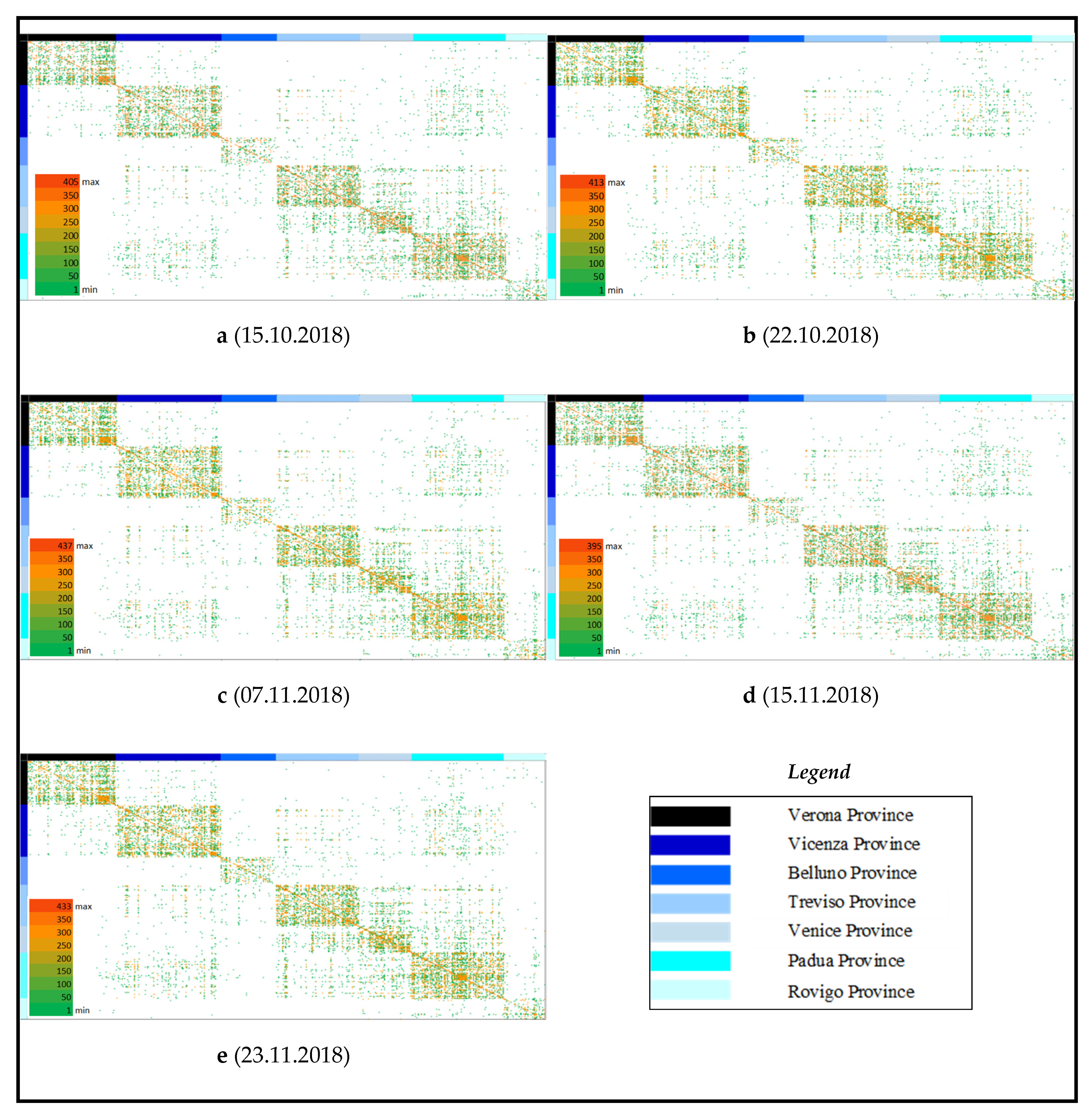
4.3. Sample O-D Matrices

Once the trips as well as their origin and destination have been defined, the following step provides their aggregation for O-D matrix building. To model the system, the study area (and possibly portions of the external area) was subdivided (Section 3.2) into a number of discrete geographic units called traffic analysis zones (TAZs). The zones were defined on the basis of official administrative areas called ACE (census areas), which are the aggregation of the census geographic units and are defined by the Italian National Institute of Statistics (ISTAT). This allows each zone to be associated with the statistical data (population, employment, etc.) usually available for such areas. In all, 675 TAZs related to 574 municipalities were identified. Therefore, for each sampling day, the O-D matrix was built; Figure 3 reports the internal (i.e., both origin and destination within the Veneto region) daily trips by car. Each province is coloured differently to describe the structure of the O-D matrices formed. To assess the range of the volume of flows on each O-D pair od, temperature diagram patterns were used. The empty cells in the O-D matrices are marked in white.

From preliminary analysis of the O-D matrices shown in Figure 3, the prevalence of intra-province trips emerges (Figure 4), as well as in the O-D flow patterns reported by ISTAT (

Table 4. Average yearly share of O-D flows by car from census data (source: ISTAT [71]).

SWod	Verona	Vicenza	Belluno	Treviso	Venice	Padua	Rovigo	Total
Verona	97.05%	2.18%	0.00%	0.05%	0.08%	0.42%	0.22%	100.00%
Vicenza	1.28%	94.37%	0.08%	1.08%	0.14%	3.02%	0.03%	100.00%
Belluno	0.01%	0.24%	96.83%	2.62%	0.16%	0.14%	0.00%	100.00%
Treviso	0.04%	2.01%	0.57%	89.76%	5.43%	2.18%	0.01%	100.00%
Venice	0.13%	0.48%	0.04%	8.35%	79.90%	10.41%	0.69%	100.00%
Padua	0.90%	4.77%	0.03%	2.35%	4.65%	85.88%	1.42%	100.00%
Rovigo	2.22%	0.27%	0.02%	0.11%	2.42%	6.50%	88.46%	100.00%
SPd	19.04%	20.20%	4.43%	19.54%	13.06%	19.36%	4.37%	100.00%

). On analysing the results plotted in Figure 5, the low variability in terms of spatial distribution of daily trips emerges, confirming that the surveyed trips are mainly systematic.

The results obtained from the sample show two main empirical findings:

• The predominance of intra-province trips;
• The O-D matrices reproduce quite well the spatial distribution revealed by ISTAT with very limited daily variation.

Calculating the difference (${\Delta }_{od}$) between the province-based O-D matrices ($S{W}_{od}^{sample}$) shown in Figure 4 with that of ISTAT ($S{W}_{od}^{ISTAT}$; Table 4):

$${\Delta }_{od}=S{W}_{od}^{ISTAT}-S{W}_{od}^{sample}$$

(6)

little difference emerges between the O-D flows structure in the sample and wider population. The calculated values of ${\Delta }_{od}$ are within the small interval. This empirically indicates the similarity of the sampling data with the real picture of car activity within the Veneto region.

Based on these initial results, below, the analysis is detailed to identify the features for reproducing O-D coverage as well as inferring trip chains in terms of number of stops.

Spatial coverage of O-D flows and trip characteristics

Attention was paid to evaluate the spatial coverage of the O-D sampling trips as well as the variability during the five days of the investigation.

Table 5. Coefficients of variation on O-D pairs of trips for the five survey days.

Province of Origin	Parameter	Province of Destination
		Verona	Vicenza	Belluno	Treviso	Venice	Padua	Rovigo
Verona	No. of O-D pairs	0.02	0.11	0.00	0.26	0.34	0.09	0.21
	Average O-D trip value	0.02	0.03	0.00	0.00	0.00	0.03	0.02
Vicenza	No. of O-D pairs	0.13	0.02	0.45	0.07	0.23	0.03	0.30
	Average O-D trip value	0.02	0.03	0.06	0.04	0.02	0.04	0.00
Belluno	No. of O-D pairs	0.71	0.10	0.05	0.06	0.24	0.18	n.a.
	Average O-D trip value	0.00	0.00	0.03	0.03	0.00	0.00	n.a.
Treviso	No. of O-D pairs	0.39	0.07	0.02	0.02	0.06	0.03	0.57
	Average O-D trip value	0.00	0.04	0.04	0.02	0.01	0.05	0.00
Venice	No. of O-D pairs	0.31	0.24	0.32	0.05	0.02	0.04	0.16
	Average O-D trip value	0.00	0.02	0.00	0.02	0.03	0.02	0.07
Padua	No. of O-D pairs	0.12	0.04	0.28	0.05	0.05	0.02	0.08
	Average O-D trip value	0.03	0.04	0.04	0.03	0.02	0.01	0.03
Rovigo	No. of O-D pairs	0.13	0.27	n.a.	1.41	0.16	0.10	0.02
	Average O-D trip value	0.10	0.00	n.a.	0.00	0.14	0.02	0.05

n.a. = not available/not applicable.

reports the coefficient of variation (CV) of the number of O-D pairs with at least one trip revealed and the average number of daily O-D trips. It can be seen that these values are quite low, confirming the highly systematic nature of the demand flows. The CV is less than 0.05 for all intra-province O-D flows, which suggests high stability in trip patterns.

Thus, attention was paid to the following travel patterns: single direct or trip chains. In a single direct trip pattern, a vehicle makes only one intermediate stop to perform any activity, while a trip chain involves multiple single direct trips from the base (home) location. In the investigated dataset, the average number of trips is four, with two stops being the highest share of trip chains. The above result is fairly constant during the survey days, as shown in Figure 6 and

Table 6. Basic statistical attributes of trip chains.

Sampling/Surveyed Days	Number of Trips Made by One Vehicle				Number of Estimated Vehicles
	Mean	Standard Deviation	Min	Max
15.10.2018	3.98	1.51	1	19	16,760
22.10.2018	4.02	1.52	1	16	16,674
07.11.2018	4.10	1.46	1	17	16,958
15.11.2018	4.16	1.47	1	16	17,139
23.11.2018	4.28	1.49	1	16	17,427

.

Our descriptive analysis of the trip chains in question reveals the predominance of even values for the number of trips made by a car in one day, confirming the systematic, home-based nature of the trips in question: the number of daily trips most frequently undertaken by the sampled cars was two (20.36%) or four (19.17%). Although the trip purpose was not known in advance, the revealed shares indicate (suggest) the predominance of “home–work–home” and “home–work–shopping/pleasure–home” trips, as shown by other studies such as Jiang et al. [73] and Vrtic et al. [19]. These findings could steer further analysis with a view to inferring trip purpose from such data combined with land use data.

4.4. Expansion to the Universe of Investigation

According to the empirical evidence summarised above, a further step concerns estimating O-D demand flows. Given the empirical representativeness of the sample in terms of province, and assuming that the sample does not contain a systematic distortion of the information provided, the procedure presented in Section 3.3 was applied. The stratum (or group of vehicles) k is represented by vehicles registered in the same province. Then, once the sampled and total population of each stratum are known, the sampling rate α_k may be obtained.

4.5. O-D Matrix Validation

This section reports the results of the verification performed through application of the O-D demand flow estimation procedure presented in an earlier section. The aim of the application was to test the ability of the above procedure to reproduce revealed road link flows. A large sample of automated traffic counts was available in the Veneto region as shown in Figure 7, comprising traffic counts on several motorways and main roads, allowing us to characterize flows in terms of vehicle numbers during 13 working days.

Hence, statistical performance is measured by the “divergence” between the estimates f* (road flow vector whose elements, $f_l^{*}$, are calculated assigning to the network the O-D flows calculated through Equations (3) and (4)) and the true road link vector f, whose element is f_l. The mean square error between the two demand vectors, MSE(f*,f), is one of the most commonly used divergence measures:

$$MSE\left(\mathit{f}\mathbf{*},\mathit{f}\right)=\frac{1}{m_l}{\displaystyle \sum _l{\left(f_l^{*}-f_l^{}\right)}^2}$$

(7)

where m_l is the number of road links.

An alternative measure is the ratio between the square root of the mean square error and average link flow, which is analogous to the coefficient of variation of a random variable:

$$RMSE=\frac{\sqrt{MSE\left(\mathit{f}\mathbf{*},\mathit{f}\right)}}{{\displaystyle \sum _l{f}_l}/m_l}.$$

(8)

Obviously, the lower the MSE and RMSE, the better the estimator f*.

Table 7. Link flow estimation: accuracy of estimates.

Type of Estimation	MSE	RMSE	MAE
Through AVM/FCD data	74	5507	3104
Updating using traffic counts	74	5489	3040

summarises the mean square error (MSE) and the ratio between the square root of the mean square error and the average demand (RMSE) calculated, while Figure 8 reports a comparison between the revealed and estimated vehicle link flows. The estimates are slightly scattered. However, the model yields good results, especially because the results are less fluctuating. Then, further analyses were developed in order to verify the dispersion of estimates.

The results plotted in Figure 8 show the modelled and observed link flows for road sections available in the Veneto region and summarises the estimation accuracy. The ordinate and the abscissa have the same scale, in which case goodness of forecast is represented by any point on the 45-degree line for which forecast=observed. Then, the 45-degree line is drawn to facilitate interpretation of the scatter plots and can reveal several forecasting characteristics: the estimates are slightly scattered, and the model reproduces actual link flows quite well. Correspondence between the regression line and the 45-degree line can be considered simply the measure of reliability. A comparison of the orientation of the regression lines and the 45-degree lines gives a visual representation of the relative quality of the forecasts: the goodness of fit is quite high, with a value of 0.96 (link flows), showing that the model yields good results, particularly, as stated above, because the results are less fluctuating.

Therefore, the procedure to improve the estimates of present O-D demand flows by combining the FCD/AVM estimator with traffic counts was implemented (Cascetta [20]):

$$d^{*}=\underset{x\ge 0}{\arg \min }\left[z_1\left(\mathrm{x},\hat{d}\right){+\mathrm{z}}_2\left(\mathrm{v}\left(\mathrm{x}\right),\hat{f}\right)\right]$$

(9)

where x is the unknown demand vector. The two functions z₁(x, $\hat{d}$) and z₂(v(x), $\hat{f}$) are the “distance” measures: z₁ measures the “distance” of the unknown demand x from the a priori estimate $\hat{d}$ (from AVM data) and z₂ measures the “distance” of the flows v(x) obtained by assigning x to the network from the traffic counts $\hat{f}$. Thus, the problem is to search the vector d* that is closest to the a priori estimate $\hat{d}$, and, once it is assigned to the network, produces the flows v(d*) closest to the counts $\hat{f}$. The results of this step are summarised in Table 7 and Figure 9, proving the limited increase in performance (less than 3%) that can be obtained. The accuracy of estimates through AVM/FCD in reproducing the current origin–destination matrix is shown. This is also evidenced by the small difference (about 1%) between the expanded matrix and estimation with traffic counts. The results discussed in this section were obtained with a reasonable computational cost, i.e., about 20 s using a routine implemented within a commercial macrosimulation tool (running in a Windows environment) through a PC desktop with Intel(R) Core(TM) i7-9700F CPU @ 3.00 GHz and 32 GB of RAM. The routine time includes the computational times for estimating the initial network costs and for running the updating procedure of Equation (9). Such a performance opens new opportunities for its integration within real-time procedures. In fact, the real-time traffic counts coming from the network could feed such a proposed procedure for producing real-time (e.g., updated every 15 min) and dynamic O-D matrices.

Further analyses are in progress to verify the dispersion of estimates, developing models according to departure time and trip purpose, and including other socio-economic data in sampling estimators.

4.6. The Road Ahead and Open Research Challenges

The goodness of the results obtained provides indications for further development, especially on the statistical significance of the estimates that can be obtained by using such data. As shown in Cascetta [20], Ortúzar and Willumsen [51], Tsekeris and Tsekeris [74], and references therein quoted, estimation of current and future O-D demand flows can require user/driver-based surveys for obtaining travel-related data (e.g., destination, activity purpose, departure time), which are resource (time and money) consuming. As recalled in the previous sections, they require, for example, the driver to stop the vehicle and answer some questions posed by the surveyor or other types of interviews performed by phone or face-to-face at home, in the office or at the transportation terminal. Nowadays, thanks to the opportunity offered by telematics, FCD/AVM data allow vehicle movements to be tracked passively. As happens with commercial vehicles [21,36]; whereby it is not uncommon for freight fleet owners to track their vehicles using fleet tracking services with the aim of locating their assets, planning routes, and monitoring vehicle and driver productivity, private vehicles are currently monitored for insurance purposes or to provide extra travel services. Vehicle tracking can reveal routes taken, tours, and stops made, and it has been widely used to ascertain user travel movements as well as easily obtain the shares/probabilities of routes chosen [61], providing an opportunity to have timely data. Above, the results obtained by analysing a large dataset of private vehicles operating in the Veneto region were described. They allow travel patterns to be identified and guide specification of O-D flow estimation; in the future, this will be extended to the route chosen and the calibration and verification of route choice modelling.

However, in order to exploit the opportunity offered by such data, their representativeness and especially their penetrations need to be determined. Below, the unresolved issues in terms of sample size and number of survey days (which help to point out daily variation as well as systematic travel activity) are discussed on the basis of the data from the Veneto region.

4.6.1. Sample Size

Estimation of sample size can be performed following traditional approaches to O-D surveys under conditions of population stratification [20,50,51,52]. As hypothesised in such studies, it is reasonable to assume that each stratum consists of a province within the study area (seven strata in the Veneto region). As part of the sampling process, representative numbers of cars to be observed during the day within some areas (provinces) are to be determined.

When identifying the sample, it should be borne in mind that not all cars randomly included in the sample can undertake a trip during the survey day. In this case, we can construct the confidence interval to predict the fluctuations of the active cars. Given a generic province o, having the number of sampled vehicles travelling (VT) during each survey day (s) and statistical data from the public authorities (e.g., ISTAT), the confidence interval for active cars can be estimated as follows:

$${\overline{VT}}_o-{\gamma }_{\alpha /2}\cdot \frac{{\sigma }_{V{T}_o}}{\sqrt{S_o}}\le {\mu }_o\le {\overline{VT}}_o+{\gamma }_{\alpha /2}\cdot \frac{{\sigma }_{V{T}_o}}{\sqrt{S_o}}$$

(10)

where

• ${\overline{VT}}_o$ is the mean of VT for province o;
• ${\mu }_o$ is the estimated mean of the travelling vehicles VT_o;
• ${\gamma }_{\alpha /2}$ is the quantile of the distribution (under Prob = 0.95 equals 1.96);
• ${\sigma }_{VTo}$ is the sample standard deviation for VT_o;
• S_o is the number (days) of observations for VT_o.

Then, using the daily O-D trips by car between provinces in the survey days, the statistical characteristics on observed O-D flows (e.g., average number of trips made by vehicles between zones—provinces, variance, and coefficient of variation) can be evaluated.

Subsequently, according to the sample size definition by Cascetta [20] and Ortúzar and Willumsen [51], given a province-based zoning and all the O-D pairs od representing the trips between or within the provinces (i.e., exchange, crossing and internal province-based trips), the number of cars ($n_{od(s)}^{cars}$) that should be monitored for O-D pair od according to sampling statistics data in day s can be calculated as follows:

$$n_{od(s)}^{cars}=\frac{100\cdot {\gamma }_{\alpha /2}^2\cdot {\sigma }_{\omega \left(s\right)}^2}{{\left(0.05\cdot {\overline{\omega }}_{\left(s\right)}\right)}^2\cdot \overline{{\tau }_s}\cdot \left(\overline{V{T}_{od}}-{\gamma }_{\alpha /2}\cdot \frac{{\sigma }_{V{T}_{od}}}{\sqrt{S_{od}}}\right)}=\frac{40000\cdot {\gamma }_{\alpha /2}^2\cdot C{V}_{\omega \left(s\right)}^2}{\overline{{\tau }_s}\cdot \left(\overline{V{T}_{od}}-{\gamma }_{\alpha /2}\cdot \frac{{\sigma }_{V{T}_{od}}}{\sqrt{S_{od}}}\right)}$$

(11)

$${\overline{\omega }}_{(s)}=\frac{{\displaystyle \sum _{o=1}^{M_{(s)}}{\displaystyle \sum _{d=1}^{W_{(s)}}{\omega }_{od(s)}}}}{M_{o(s)}\cdot W_{o(s)}}$$

(12)

where

• $n_{od(s)}^{cars}$ is the number of cars that should be monitored for O-D pair od according to sampling statistics data in day s;
• ${\overline{\omega }}_{\left(s\right)}$ is the average number of trips made by vehicles between or within provinces during the observation day s;
• ${\sigma }_{{\omega }_{\left(s\right)}}^2$ is the variance of number of trips made by vehicles between or within provinces during the observation day s;
• $C{V}_{{\omega }_{o(s)}}^2$ is the coefficient of variation of number of trips made by vehicles between or within provinces during the observation day s;
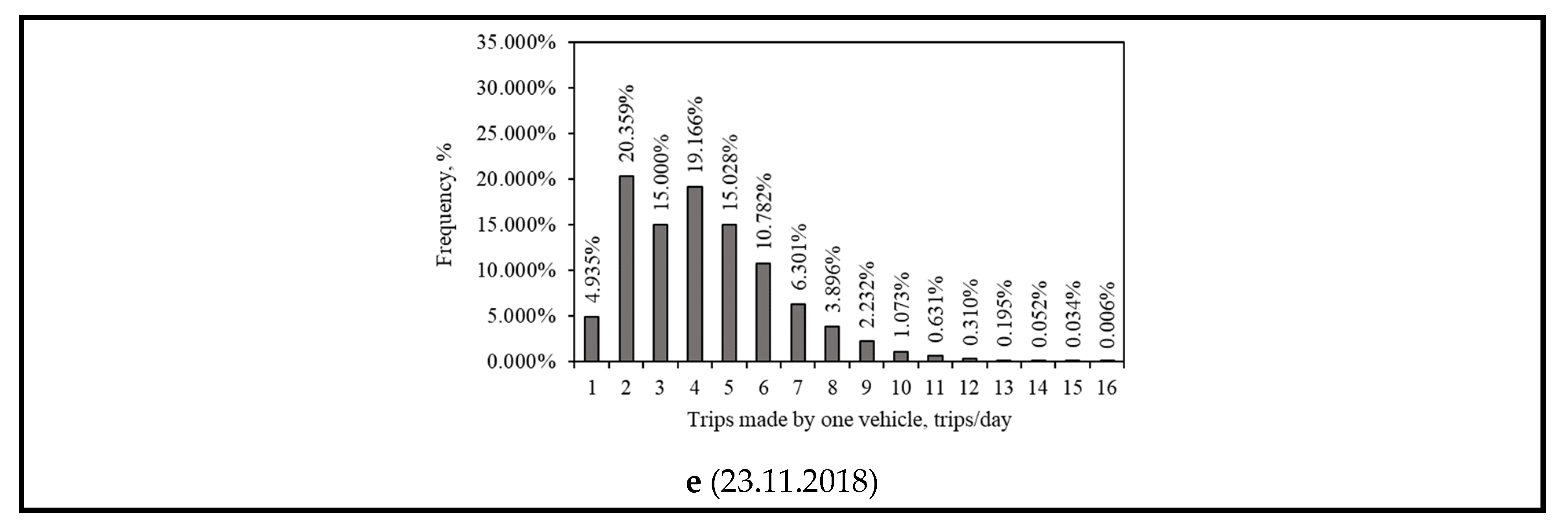
• $\overline{{\tau }_s}$ is the average number of trips made by one vehicle during day s;
• ${\omega }_{od(s)}$ is the detected (revealed) flow between zone o and zone d between or within the provinces in survey (observation) day s;
• $M_{o(s)}$ is the detected number of origin zones in day s for province o;
• $W_{o(s)}$ is the detected number of destination zones in day s for province o.

Equation (11) allows us to obtain the number of cars that should be monitored from every province-based O-D pair. Such values should guarantee the representativeness of the necessary sample. However, given that it could be operatively easier to obtain information on the start place of travel and since Equation (4) gives the matrix results, the minimum number of vehicles to monitor should refer to the origin. Therefore, the necessary sample of vehicles (cars) for province o in a day s, $n_{o(s)}^{cars}$, can be obtained as follows:

$$n_{o(s)}^{cars}={\displaystyle \sum _d{n}_{od(s)}^{cars}}$$

(13)

where the sum is extended to all possible destinations d of the study reached by trips starting from origin (province) o.

As the FCD/AVM data could be easily obtained for more than one day, the number of the sampled cars, taking into account several days of observations (S), can be evaluated as follows:

$$n_o^{cars}=\mathrm{m}\underset{s}{a}x\left(n_{o(s)}^{cars}\right), s\in [1,\dots ,S]$$

(14)

where $n_o^{cars}$ is the final sample size of cars that should be monitored from zone (province) o.

4.6.2. Sampling Days

The next step to determine sample size could be to evaluate the minimum number of surveyed days in order to infer the spatialization of O-D patterns. A possible methodology could be based on the estimation procedure for O-D flow values among survey days. Thus, if the trip patterns are relatively stable during the survey days, we can reduce the monitoring days without any negative consequences for the data obtained. To do this, the variability of the O-D flows within S survey days can be evaluated as follows. With the statistics data on observed sampled trips, i.e., average O-D flows ${\varphi }_{od}$ within S days, and its variance ${\sigma }_{od(\varphi )}^2$, the number of survey days required for every O-D pair od can be found according to Ortúzar and Willumsen [54] as follows:

$$n_{od}^{days}=\frac{{\gamma }_{\alpha /2}^2\cdot {\sigma }_{od(\varphi )}^2}{{\left(0.05\cdot {\varphi }_{od}\right)}^2}=1536\cdot C{V}_{od(\varphi )}^2$$

(15)

$${\varphi }_{od}=\frac{{\displaystyle \sum _{s=1}^S{\overline{\omega }}_{{}_{od}(s)}}}{S}$$

(16)

where

• $n_{od}^{days}$ is the number of survey days required for the flows between zones (provinces) o and d;
• ${\varphi }_{od}$ is the average value of flows on O-D pair od within S days;
• ${\sigma }_{od(\phi )}^2$ is the variance of flows on O-D pair od within S days;
• ${\overline{\omega }}_{{}_{od}(s)}$ is the average O-D flow between zone (province) pair od for the survey day s.

Equation (15) gives the number of the survey days needed for the representative sample for every O-D pair considered. In this case, for every origin zone (province) o, several numbers of $n_{od}^{days}$ can be obtained. Therefore, the final number of survey days for each study zone (province) can be obtained as follows:

$$n_o^{days}=\mathrm{m}\underset{d}{a}x\left(n_{od}^{days}\right), d\in [1,\dots ,P]$$

(17)

where $n_o^{days}$ is the quantity of survey days required for zone (province) o, and P is the total number of zones (provinces) in the O-D matrix.

4.6.3. Example of Application to the Veneto Region

The data reported in Table 1 and Table 3 allow the percentage of VT during the survey days to be obtained (

Table 8. Data on VT values for the observation days.

Province of Vehicle Registration	VT [%]					Mean [%]	Standard Deviation [%]	Confidence Interval
	15.10	22.10	07.11	15.11	23.11			Left Side [%]	Right Side [%]
Belluno	48.91	48.04	48.91	50.22	48.04	48.82	0.80	48.12	49.52
Padua	58.92	58.80	59.64	60.58	58.80	59.35	0.69	58.75	59.95
Rovigo	56.19	56.19	56.67	55.95	56.19	56.24	0.24	56.03	56.45
Treviso	64.00	63.78	64.75	65.23	63.78	64.31	0.58	63.80	64.82
Venice	46.4	46.24	46.21	47.83	46.24	46.58	0.63	46.03	47.13
Verona	58.11	57.70	58.68	59.12	57.70	58.26	0.56	57.77	58.75
Vicenza	56.54	56.06	57.66	57.71	56.06	56.81	0.74	56.16	57.46

). The left side of the confidence interval will reflect the lowest predicted percentage of the vehicles that would travel with a confidence threshold of 0.95. This information is taken into account when the necessary sample sizes are estimated according to Equations (11)–(14).

The estimated sizes of the representative samples for the provinces are presented in Figure 10. The calculation was made under two conditions: all monitored cars would travel during the day (VT = 100 %) and the real conditions of the monitored vehicles’ activity, i.e., when not all cars monitored in a day would make a trip (VT < 100%, data from Table 8). An error forecast at 5% was assumed. As indicated by Figure 10, the goodness of the results obtained in reproducing observed link flows can be explained by the fact that all provinces were covered with a larger quantity of observed vehicles than the representative samples required.

Subsequently, a research challenge in using FCD/AVM data would be to find the minimum number of sampling days required. The calculations can be made through Equations (15)–(17). The results are presented in

Table 9. The resulting data of the required number of survey days.

Province of Origin	Province of Destination							Required No. of Survey Days
	Verona	Vicenza	Belluno	Treviso	Venice	Padua	Rovigo
Verona	1	1	1	1	1	1	1	1
Vicenza	1	1	5	2	1	2	1	5
Belluno	1	1	1	1	1	1	n.a.	1
Treviso	1	3	3	1	1	4	1	4
Venice	1	1	1	1	1	1	8	8
Padua	1	3	3	1	1	1	1	3
Rovigo	14	1	n.a.	1	31	1	5	31

n.a. = not available/not applicable.

.

The results reported in Table 8 indicate that necessary days of observation for Verona, Vicenza, Belluno, Treviso, and Padua provinces are less or equal to five. Only Venice and Rovigo provinces need more than five days of investigation, i.e., 8 and 31, respectively. This may be explained by a large variance in average O-D trip values between Rovigo–Verona, Rovigo–Venice, and Venice–Rovigo. The O-D flows between these O-D pairs are not stable within weekdays. With reference to Figure 4, it may be seen that $S{W}_{od}$ vary for Rovigo–Verona from 1.62% to 2.35%, Rovigo–Venice from 1.28% to 1.96%, and Venice–Rovigo from 0.17% to 0.24%, reflecting the specific weight in the total trip values generated by the provinces. If the O-D flows with the highest specific weight are considered (the intra-province trips), in this case, the number of days required does not exceed five. Accordingly, it may be concluded that five survey days gave representative information on O-D flows within the study area.

5. Conclusions

The paper presented recent developments in O-D flow estimation through AVM/FCD, hence dealing with link flows to be forecast and road network performance to be assessed. We reviewed the main modelling approaches to be implemented in order to estimate the O-D daily flows through the new opportunities offered by telematics, presented some analyses to exploit the opportunities offered by AVM data capable of identifying and assessing car patterns, and tested the estimation framework through comparison with traffic counts.

The first part of the paper gave an overview of the procedures developed and presented an estimation procedure to obtain car O-D flows using an aggregate approach; the second part reported evidence on trips/trip chains performed by cars belonging to a large dataset, which operate in the Veneto region, followed by the validation/verification results. This allowed mechanisms for driving trip generation to be captured more accurately and a trip chain order to be reproduced.

The proposed O-D estimation procedure was structured into three levels: car trip identification, sample O-D matrix, O-D (i.e., expansion to the universe of investigation). The car trip identification procedure was implemented in order to obtain the trips, and hence trip chains, for each surveyed vehicle. The sample O-D matrix was obtained by means of a trip-grouping procedure, and the result was compared with a sample O-D matrix available for census, revealing little difference between them. The expansion to the universe made it possible to obtain the average O-D matrix for the study area. In order to validate this result, the matrix was assigned, and the flows were compared with available traffic counts on a subset of links, showing low differences among them.

These results indicate that AVM/FCD allow us to have an estimate of O-D demand flows and reproduce quite well the critical patterns along roads. In addition, they enable us to provide a continuous picture of the network status as well as exploit the potential of data-driven approaches for simulating transportation systems. Vehicle activity pattern identification is crucial to characterise passenger operations from AVM/FCD/GPS data. The results of this paper show the potential of the proposed procedure to identify vehicle trips as well as characterise demand flows spatially. Future work will focus on testing and calibrating the procedure with passenger diary data, to assess its efficacy in detecting stops of very short duration and identify passenger activity. With the growing availability of data, there is great potential for the use of this procedure to characterise passenger trips and as a tool in transportation planning in general.

The proposed methodology of O-D matrix sample estimation may be used for urban and interurban transportation policy making. The field of application is huge, covering attributes of urban logistics [75,76,77], determining mobility patterns for the sustainable development of metropolitan areas and intercity road connections [78,79]. Current trends and challenges for future mobility based on electric automated vehicles [80,81] and carsharing services [82] need to be anticipated. The efficient operation of such systems cannot be implemented without robust data on trip chain formation. As one of the ways to achieve this goal, we propose to estimate trip behaviour using AVM/FCD/GPS data with the sampling survey option.

Although the obtained statistics confirm the value of the proposed approach, further developments are in progress to improve the results and apply more advanced machine learning techniques that allow further features to be included in model specification and in modelling accuracy. The modelling framework that can be developed exploiting AVM/FCD could benefit from investigation of the influence of socio-economic attributes on tour/trip chain definition, the inclusion of the size function in delivery location choice, modelling of the choice set generation within the delivery location model, and inclusion of departure time choice in order to investigate the relationship with time-window access restrictions in progress.

References

1. Axhausen, K.W.; Zimmermann, A.; Schönfelder, S.; Rindsfüser, G.; Haupt, T. Observing the rhythms of daily life: A six-week travel diary. Transport 2002, 29, 95–124. [Google Scholar] [CrossRef]
2. Ben-Akiva, M. Structure of Passenger Travel Demand Models. Ph.D Thesis, Massachusetts Institute of Technology, Cambridge, MA, USA, 1973; 268p. [Google Scholar]
3. Hensher, D.A. Stated preference analysis of travel choices: The state of practice. Transport 1994, 21, 107–133. [Google Scholar] [CrossRef] [Green Version]
4. Kitamura, R.; Mokhtarian, P.L.; Daidet, L. A micro-analysis of land use and travel in five neighborhoods in the San Francisco Bay Area. Transport 1997, 24, 125–158. [Google Scholar] [CrossRef]
5. McFadden, D. The measurement of urban travel demand. J. Public Econ. 1974, 3, 303–328. [Google Scholar] [CrossRef]
6. Schlich, R.; Axhausen, K.W. Habitual travel behaviour: Evidence from a six-week travel diary. Transport 2003, 30, 13–36. [Google Scholar] [CrossRef]
7. Williams, H.; Ortuzar, J. Behavioural theories of dispersion and the mis-specification of travel demand models. Transp. Res. Part B Methodol. 1982, 16, 167–219. [Google Scholar] [CrossRef]
8. Wilson, A. A statistical theory of spatial distribution models. Transp. Res. 1967, 1, 253–269. [Google Scholar] [CrossRef]
9. Alonso, B.; Moura, J.L.; Ibeas, Á.; dell’Olio, L. Using O–D matrices for decision making in road network management. Transport 2013, 28, 31–37. [Google Scholar] [CrossRef]
10. Bierlaire, M. The total demand scale: A new measure of quality for static and dynamic origin–destination trip tables. Transp. Res. Part B Methodol. 2002, 36, 837–850. [Google Scholar] [CrossRef]
11. Cascetta, E.; Postorino, M.N. Fixed point approaches to the estimation of O/D matrices using traffic counts on congested networks. Transp. Sci. 2001, 35, 134–147. [Google Scholar] [CrossRef]
12. Foulds, L.R.; Nascimento, H.A.D.; Calixto, I.; Hall, B.R.; Longo, H. A fuzzy set-based approach to origin–destination matrix estimation in urban traffic networks with imprecise data. Eur. J. Oper. Res. 2013, 231, 190–201. [Google Scholar] [CrossRef]
13. Hazelton, M. Some comments on origin–destination matrix estimation. Transp. Res. Part A Policy Pract. 2003, 37, 811–822. [Google Scholar] [CrossRef]
14. He, B.Y.; Chow, J.Y.J. Gravity Model of Passenger and Mobility Fleet Origin–Destination Patterns with Partially Observed Service Data. Transp. Res. Board 2021. [Google Scholar] [CrossRef]
15. Iqbal, M.S.; Choudhury, C.F.; Wang, P.; González, M.C. Development of origin–destination matrices using mobile phone call data. Transp. Res. Part C Emerg. Technol. 2014, 40, 63–74. [Google Scholar] [CrossRef] [Green Version]
16. Mitra, A.; Attanasi, A.; Meschini, L.; Gentile, G. Methodology for O-D matrix estimation using the revealed paths of floating car data on large-scale networks. IET Intell. Transp. Syst. 2020, 14, 1704–1711. [Google Scholar] [CrossRef]
17. Munizaga, M.A.; Palma, C. Estimation of a disaggregate multimodal public transport Origin–Destination matrix from passive smartcard data from Santiago, Chile. Transp. Res. Part C Emerg. Technol. 2012, 24, 9–18. [Google Scholar] [CrossRef]
18. Russo, F.; Vitetta, A. Reverse assignment: Calibrating link cost functions and updating demand from traffic counts and time measurements. Inverse Probl. Sci. Eng. 2011, 19, 921–950. [Google Scholar] [CrossRef]
19. Vrtic, M.; Fröhlich, P.; Schussler, N.; Axhausen, K.; Lohse, D.; Schiller, C.; Teichert, H. Two-dimensionally constrained disaggregate trip generation, distribution and mode choice model: Theory and application for a Swiss national model. Transp. Res. Part A Policy Practice 2007, 41, 857–873. [Google Scholar] [CrossRef] [Green Version]
20. Cascetta, E. Transportation Systems Analysis–Models and Applications, 2nd ed.; Springer: New York, NY, USA, 2009; 742p. [Google Scholar]
21. Antoniou, C.; Dimitrou, L.; Pereira, F. Mobility Patterns, Big Data and Transport Analytics—Tools and Applications for Modelling; Elsevier: Amsterdam, The Netherlands, 2020. [Google Scholar]
22. Dixon, M.P.; Rilett, L.R. Real-time OD estimation using automatic vehicle identification and traffic count data. Comput. Civ. Infrastruct. Eng. 2002, 17, 7–21. [Google Scholar] [CrossRef]
23. Nasab, M.R.; Shafahi, Y. Estimation of origin–destination matrices using link counts and partial path data. Transport 2020, 47, 2923–2950. [Google Scholar] [CrossRef]
24. Michau, G.; Pustelnik, N.; Borgnat, P.; Abry, P.; Bhaskar, A.; Chung, E. Combining traffic counts and bluetooth data for link-origin-destination matrix estimation in large urban networks: The Brisbane case study. arXiv 2019, arXiv:1907.07495. [Google Scholar]
25. Guo, J.; Liu, Y.; Li, X.; Huang, W.; Cao, J.; Wei, Y. Enhanced least square based dynamic OD matrix estimation using radio frequency identification data. Math. Comput. Simul. 2017, 155, 27–40. [Google Scholar] [CrossRef]
26. Caceres, N.; Romero, L.M.; Benitez, F.G. Exploring strengths and weaknesses of mobility inference from mobile phone data vs. travel surveys. Transp. A Transp. Sci. 2020, 16, 574–601. [Google Scholar] [CrossRef]
27. Marra, A.D.; Becker, H.; Axhausen, K.W.; Corman, F. Developing a passive GPS tracking system to study long-term travel behavior. Transp. Res. Part C Emerg. Technol. 2019, 104, 348–368. [Google Scholar] [CrossRef] [Green Version]
28. McGowen, P.; McNally, M. 2007. Evaluating the potential to predict activity types from GPS and GIS data. In Proceedings of the Transportation Research Board 86th Meeting, Washington, DC, USA, 21–25 January 2007. [Google Scholar]
29. Widhalm, P.; Yang, Y.; Ulm, M.; Athavale, S.; González, M.C. Discovering urban activity patterns in cell phone data. Transport 2015, 42, 597–623. [Google Scholar] [CrossRef] [Green Version]
30. Wolf, J.; Guensler, R.; Bachman, W. Elimination of the travel diary: Experiment to derive trip purpose from global positioning system travel data. Transp. Res. Rec. 2001, 1768, 125–134. [Google Scholar] [CrossRef] [Green Version]
31. Alsger, A.; Tavassoli, A.; Mesbah, M.; Ferreira, L. Evaluation of effects from sample-size origin-destination estimation using smart card fare data. J. Transp. Eng. Part A Syst. 2017, 143, 04017003. [Google Scholar] [CrossRef]
32. He, L.; Agard, B.; Trépanier, M. A classification of public transit users with smart card data based on time series distance metrics and a hierarchical clustering method. Transp. A Transp. Sci. 2018, 16, 56–75. [Google Scholar] [CrossRef]
33. Peftitsi, S.; Jenelius, E.; Cats, O. Determinants of passengers’ metro car choice revealed through automated data sources: A Stockholm case study. Transp. A Transp. Sci. 2020, 16, 529–549. [Google Scholar] [CrossRef]
34. Tavassoli, A.; Mesbah, M.; Hickman, M. Calibrating a transit assignment model using smart card data in a large-scale multi-modal transit network. Transport 2019, 47, 2133–2156. [Google Scholar] [CrossRef]
35. Yap, M.; Cats, O.; van Arem, B. Crowding valuation in urban tram and bus transportation based on smart card data. Transp. A Transp. Sci. 2020, 16, 23–42. [Google Scholar] [CrossRef] [Green Version]
36. Alho, A.R.; You, L.; Lu, F.; Cheah, L.; Zhao, F.; Ben-Akiva, M. Next generation freight vehicle surveys: Supplementing truck GPS tracking with a driver activity survey. In Proceedings of the 21st IEEE International Conference on Intelligent Transportation Systems, Maui, HI, USA, 4–7 November 2018. [Google Scholar]
37. Figliozzi, M. Modeling the impact of technological changes on urban commercial trips by commercial activity routing type. Transp. Res. Rec. 2006, 1964, 118–126. [Google Scholar] [CrossRef]
38. Gonzalez-Feliu, J.; Pluvinet, P.; Serouge, M.; Gardrat, M. GPS-based data production in urban freight distribution. Glob. Position. Syst. Signal Struct. Appl. Sources Error Biases 2013, 1–20. [Google Scholar]
39. Nuzzolo, A.; Comi, A.; Papa, E.; Polimeni, A. 2019. Understanding taxi travel demand patterns through floating car data. In Data Analytics: Paving the Way to Sustainable Urban Mobility, Proceedings of the 4th Conference on Sustainable Urban Mobility (CSUM2018), Skiathos Island, Greece, 24–25 May 2018; Nathanail, E., Karakikes, I.D., Eds.; Springer: Berlin/Heidelberg, Germany, 2018; pp. 445–452. [Google Scholar] [CrossRef] [Green Version]
40. Comi, A.; Nuzzolo, A.; Polimeni, A. Aggregate delivery tour modeling through AVM data: Experimental evidence for light goods vehicles. Transp. Lett. 2021, 13, 201–208. [Google Scholar] [CrossRef]
41. Comi, A.; Polimeni, A. Forecasting delivery pattern through AVM/FCD data: Empirical evidence. Future Transp. 2021, 1, 707–719. [Google Scholar]
42. Holguín-Veras, J.; Encarnación, T.; Perez-Guzman, S.; Yang, X. Mechanistic identification of freight activity stops from global positioning system data. Transp. Res. Rec. 2020, 2674, 235–246. [Google Scholar] [CrossRef]
43. Polimeni, A.; Vitetta, A. Vehicle routing in urban areas: An optimal approach with cost function calibration. Transp. B Transp. Dyn. 2013, 2, 1–19. [Google Scholar] [CrossRef]
44. Thoen, S.; Tavasszy, L.; de Bok, M.; Correia, G.; van Duin, R. Descriptive modeling of freight tour formation: A shipment-based approach. Transp. Res. Part E Logist. Transp. Rev. 2020, 140, 101989. [Google Scholar] [CrossRef]
45. Alesio, T. Position Monitoring System and Method. U.S. Patent 5,550,551, 27 August 1996. [Google Scholar]
46. Rothert, M.F.; Janky, J.M. Automated Vehicle Monitoring System. U.S. Patent 6,141,610, 31 October 2000. [Google Scholar]
47. OnStar. OnStar: In-Vehicle Safety and Security System. 2021. Available online: https://www.onstar.com (accessed on 25 July 2021).
48. Bartlett, J.E.; Kotrlik, J.W.; Higgins, C.C. Organizational research: Determining appropriate sample size in survey research. Inf. Technol. Learn. Perform. J. 2001, 19, 43–50. [Google Scholar]
49. Bolbol, A.; Cheng, T.; Tsapakis, I.; Chow, A.H. Sample size calculation for studying transportation modes from GPS data. Procedia-Soc. Behav. Sci. 2012, 48, 3040–3050. [Google Scholar] [CrossRef] [Green Version]
50. Ceder, A. Public Transit Planning and Operation: Theory, Modelling and Practice, 1st ed.; CRC press: Boca Raton, FL, USA, 2007; 645p. [Google Scholar]
51. Ortúzar, J.D.; Willumsen, L.G. Modelling Transport, 4th ed.; John Wiley & Sons, Ltd: Hoboken, NJ, USA, 2011. [Google Scholar]
52. Smith, M.E. 1979. Design of small sample home interview travel surveys. Transp. Res. Rec. 1979, 701, 29–35. [Google Scholar]
53. Messelodi, S.; Modena, C.M.; Zanin, M.; De Natale, F.G.; Granelli, F.; Betterle, E.; Guarise, A. Intelligent extended floating car data collection. Expert Syst. Appl. 2009, 36, 4213–4227. [Google Scholar] [CrossRef]
54. Ehmke, J.F.; Meisel, S.; Mattfeld, D. Floating car based travel times for city logistics. Transp. Res. Part C Emerg. Technol. 2012, 21, 338–352. [Google Scholar] [CrossRef]
55. Rahmani, M.; Jenelius, E.; Koutsopoulos, H.N. Non-parametric estimation of route travel time distributions from low-frequency floating car data. Transp. Res. Part C Emerg. Technol. 2015, 58, 343–362. [Google Scholar] [CrossRef]
56. Rahmani, M.; Koutsopoulos, H.N.; Jenelius, E. Travel time estimation from sparse floating car data with consistent path inference: A fixed point approach. Transp. Res. Part C Emerg. Technol. 2017, 85, 628–643. [Google Scholar] [CrossRef]
57. Tu, W.; Fang, Z.; Li, Q. Exploring time varying shortest path of urban OD Pairs based on floating car data. In Proceedings of the 2010 18th International Conference on Geoinformatics, Beijing, China, 18–20 June 2010; pp. 1–6. [Google Scholar] [CrossRef]
58. Dewulf, B.; Neutens, T.; Vanlommel, M.; Logghe, S.; De Maeyer, P.; Witlox, F.; De Weerdt, Y.; Van de Weghe, N. Examining commuting patterns using Floating Car Data and circular statistics: Exploring the use of new methods and visualizations to study travel times. J. Transp. Geogr. 2015, 48, 41–51. [Google Scholar] [CrossRef]
59. Yamamoto, T.; Miwa, T.; Takeshita, T.; Morikawa, T. Updating dynamic origin-destination matrices using observed link travel speed by probe vehicles. In Transportation and Traffic Theory 2009: Golden Jubilee; Lam, W., Wong, S., Lo, H., Eds.; Springer: Boston, MA, USA, 2009; p. 723. [Google Scholar] [CrossRef]
60. Cao, P.; Miwa, T.; Yamamoto, T.; Morikawa, T. Bilevel generalized least squares estimation of dynamic origin–destination matrix for urban network with probe vehicle data. Transp. Res. Rec. J. Transp. Res. Board 2013, 2333, 66–73. [Google Scholar] [CrossRef]
61. Croce, A.; Musolino, G.; Rindone, C.; Vitetta, A. Route and path choices of freight vehicles: A case study with floating car data. Sustainability 2020, 12, 855. [Google Scholar] [CrossRef]
62. Stipancic, J.; Miranda-Moreno, L.; Saunier, N. Vehicle manoeuvers as surrogate safety measures: Extracting data from the gps-enabled smartphones of regular drivers. Accid. Anal. Prev. 2018, 115, 160–169. [Google Scholar] [CrossRef]
63. Sun, L.; Lee, D.H.; Erath, A.; Huang, X. Using smart card data to extract passenger’s spatio-temporal density and train’s trajectory of MRT system. In Proceedings of the ACM SIGKDD International Workshop on Urban Computing, Beijing, China, 12 August 2012. [Google Scholar]
64. Carrese, S.; Cipriani, E.; Mannini, L.; Nigro, M. Dynamic demand estimation and prediction for traffic urban networks adopting new data sources. Transp. Res. Part C Emerg. Technol. 2017, 81, 83–98. [Google Scholar] [CrossRef]
65. Yang, X.; Lu, Y.; Hao, W. Origin-destination estimation using probe vehicle trajectory and link counts. J. Adv. Transp. 2017, 2017, 1–18. [Google Scholar] [CrossRef]
66. Sbaï, A.; Van Zuylen, H.J.; Li, J.; Zheng, F.; Ghadi, F. Estimation of an urban OD matrix using different information sources. In Computational Science and Its Applications–ICCSA 2017. Lecture Notes in Computer Science; Gervasi, O., Ed.; Springer International Publishing: Cham, Switzerland, 2017; Volume 10405, pp. 183–198. [Google Scholar] [CrossRef]
67. Vogt, S.; Fourati, W.; Schendzielorz, T.; Friedrich, B. Estimation of origin-destination matrices by fusing detector data and Floating Car Data. Transp. Res. Procedia 2019, 37, 473–480. [Google Scholar] [CrossRef]
68. Dabbas, H.; Fourati, W.; Friedrich, B. Floating car data for traffic demand estimation-field and simulation studies. In Proceedings of the 2020 IEEE 23rd International Conference on Intelligent Transportation Systems (ITSC), Rhodes, Greece, 20–23 September 2020; pp. 1–8. [Google Scholar] [CrossRef]
69. Guo, D.; Zhu, X.; Jin, H.; Gao, P.; Andris, C. Discovering spatial patterns in origin-destination mobility data. Trans. GIS 2012, 16, 411–429. [Google Scholar] [CrossRef]
70. Tang, J.; Liu, F.; Wang, Y.; Wang, H. Uncovering urban human mobility from large scale taxi GPS data. Phys. A Stat. Mech. Its Appl. 2015, 438, 140–153. [Google Scholar] [CrossRef]
71. ISTAT. Il Veneto e la mobilità sostenibile. In Rapporto Statistico 2018; Italian Institute of Statistics: Rome, Italy, 2018. [Google Scholar]
72. ACI. Autoritratto 2018; Automobile Club d’Italia: Rome, Italy, 2019. [Google Scholar]
73. Jiang, S.; Ferreira, J.; Gonzalez, M.C. Activity-based human mobility patterns inferred from mobile phone data: A case study of Singapore. IEEE Trans. Big Data 2017, 3, 208–219. [Google Scholar] [CrossRef] [Green Version]
74. Tsekeris, T.; Tsekeris, C. Demand forecasting in transport: Overview and modeling advances. Econ. Res.-Ekon. Istraživanja 2011, 24, 82–94. [Google Scholar] [CrossRef] [Green Version]
75. Comi, A.; Delle Site, P.; Filippi, F.; Marcucci, E.; Nuzzolo, A. Differentiated regulation of urban freight traffic: Conceptual framework and examples from Italy. In Proceedings of the 13th International Conference of Hong Kong Society for Transportation Studies, Hong Kong, China, 13–15 December 2008. [Google Scholar]
76. Holguín-Veras, J.; Leal, J.A.; Sanchez-Diaz, I.; Browne, M.; Wojtowicz, J. State of the art and practice of urban freight management Part II: Financial approaches, logistics, and demand management. Transp. Res. Part A Policy Pracitce 2020, 137, 383–410. [Google Scholar] [CrossRef]
77. Nuzzolo, A.; Comi, A. A system of models to forecast the effects of demographic changes on urban shop restocking. Res. Transp. Bus. Manag. 2014, 11, 142–151. [Google Scholar] [CrossRef]
78. Banister, D. The sustainable mobility paradigm. Transp. Policy 2008, 15, 73–80. [Google Scholar] [CrossRef]
79. Tight, M.; Bristow, A.; Pridmore, A.; May, A. What is a sustainable level of CO2 emissions from transport activity in the UK in 2050? Transp. Policy 2005, 12, 235–244. [Google Scholar] [CrossRef] [Green Version]
80. Bösch, P.M.; Becker, F.; Becker, H.; Axhausen, K.W. Cost-based analysis of autonomous mobility services. Transp. Policy 2018, 64, 76–91. [Google Scholar] [CrossRef]
81. de Almeida Correia, G.H.; van Arem, B. Solving the user optimum privately owned automated vehicles assignment problem (UO-POAVAP): A model to explore the impacts of self-driving vehicles on urban mobility. Transp. Res. Part B Methodol. 2016, 87, 64–88. [Google Scholar] [CrossRef]
82. Mishra, G.S.; Clewlow, R.R.; Mokhtarian, P.L.; Widaman, K.F. The effect of carsharing on vehicle holdings and travel behavior: A propensity score and causal mediation analysis of the San Francisco Bay Area. Res. Transp. Econ. 2015, 52, 46–55. [Google Scholar] [CrossRef]
Figure 1. The proposed methodology.
Information 12 00493 g001
Figure 2. Structure of the AVM/FCD database.
Information 12 00493 g002
Figure 3. Veneto O-D matrices for the five survey days.
Information 12 00493 g003
Figure 4. Shares of O-D flows between provinces of the Veneto region (sample-based).
Information 12 00493 g004
Figure 5. Comparison of O-D flows specific weight between sampling and ISTAT data.
Information 12 00493 g005
Figure 6. Distribution of daily trip number made by sampled vehicles.
Information 12 00493 g006aInformation 12 00493 g006b
Figure 7. Traffic counts available in the Veneto region (background source: OpenStreetMap).
Information 12 00493 g007
Figure 8. Comparison between revealed and modelled road link flows.
Information 12 00493 g008
Figure 9. Comparison between revealed and modelled road link flows (after updating).
Information 12 00493 g009
Figure 10. Samples of monitored vehicle numbers under different conditions of activity.
Information 12 00493 g010