
Classification of Relaxation and Concentration Mental States with EEG


Department of Computer Science and Information Engineering, National Taipei University of Technology, Taipei 106344, Taiwan
Information 2021, 12(5), 187; https://0-doi-org.brum.beds.ac.uk/10.3390/info12050187
Submission received: 15 March 2021
/
Revised: 15 April 2021
/
Accepted: 23 April 2021
/
Published: 26 April 2021
(This article belongs to the Special Issue ICCCI 2020&2021: Advances in Baseband Signal Processing, Circuit Designs, and Communications)
Abstract
:In this paper, we study the use of EEG (Electroencephalography) to classify between concentrated and relaxed mental states. In the literature, most EEG recording systems are expensive, medical-graded devices. The expensive devices limit the availability in a consumer market. The EEG signals are obtained from a toy-grade EEG device with one channel of output data. The experiments are conducted in two runs, with 7 and 10 subjects, respectively. Each subject is asked to silently recite a five-digit number backwards given by the tester. The recorded EEG signals are converted to time-frequency representations by the software accompanying the device. A simple average is used to aggregate multiple spectral components into EEG bands, such as , , and bands. The chosen classifiers are SVM (support vector machine) and multi-layer feedforward network trained individually for each subject. Experimental results show that features, with bands and bandwidth 4 Hz, the average accuracy over all subjects in both runs can reach more than 80% and some subjects up to 90+% with the SVM classifier. The results suggest that a brain machine interface could be implemented based on the mental states of the user even with the use of a cheap EEG device.
1. Introduction
Inputting information to a machine solely based on “thoughts” of the brain is a long-seeking goal to communicate with machines. Furthermore, known as brain–computer interface (BCI), this technique is especially useful when the user is unable to use hands to control the machine or choose the options the machine provides. Among the brain–computer interface techniques, a widely used one is through analyzing the EEG (Electroencephalography) signals of the user. Typically, the EEG signal is divided into several bands, including delta () band for frequency less than 4 Hz, theta () band for 4–7 Hz, alpha () band for 8–12 Hz, beta () band for 13–30 Hz, and gamma () band for frequencies higher than 30 Hz [1]. In terms of application, when a person is relaxed, the power in alpha band is stronger; whereas when a person concentrates their attention, the beta band will have a stronger power [2].
Although detecting a person’s mental states by classifying an EEG signal has been studied for many years, many existing papers reported the results based on instrumental EEG (recording) devices, which are capable of recording many channels [1,3,4,5,6]. However, an instrumental EEG device is expensive. In order to use the EEG device for BCI in a commercial market, this device must be affordable. In this paper, we use a low-cost (less than 300 USD) EEG device from Neurosky. In contrast to an instrumental EEG device, a cheap device typically has only one or two channels to minimize the cost. Therefore, we need to perform classification based on one or two channels. It is then import to study whether one or two channels are sufficient to obtain high accuracy in actual applications. After reading some existing literature, the answer seems inconclusive, some with good accuracy [7,8], high correlation [9], or acceptable usability [10], whereas others with extremely low accuracy [11] or marginal accuracy (around 50%) [12]. Therefore, we intend to find out our own answer.
To invoke two mental states for classification, we initially recorded EEG for subjects listening to favorite or dislike songs. We later found that the accuracy was strongly affected by the selected song titles for each subject. We then concluded that mental states invoked by listening to favorite songs was not a reliable choice. Therefore, we decided to classify only attention and meditation states. This problem has been studied by many researchers before, e.g., [5,6,7,8,9,10,11,12,13,14,15]. Although such a problem is a binary classification problem, it is actually not easy to achieve high accuracy. For example, the accuracy of [11] is around 60% even with the use of a 14-channel EEG device. In Section 2, we will review some existing work and provide the reported accuracy. Overall, to improve the classification accuracy, it is important to have a method to invoke these two states with high accuracy.
As pointed out by Kahneman in [16], when a person is doing effortful work, their pupils dilate substantially. With this kind of physiological evidence, we think that it could be easier to classify the metal states as effortful or effortless states with a low-cost EEG device. In the following, we use concentrated state to mean that a person’s mind is doing effortful work and relaxed state if not doing effortful work. In the literature, some authors use attention state and meditation state to represent similar mental states as ours presented here. Because we intend to develop an efficient mechanism to communicate with the machine, it is acceptable to pick any type of mental state as the input to the machine. Though there are only two mental states considered in this paper, it is still possible to develop a user interface with only two options. For example, we can associate “yes” with the concentrated state and “no” with the relaxed state. Thus, the key issue of the technique is how to identify these two states with sufficient accuracy in a reasonable time using a cheap EEG recording device.
The contributions of this paper include (please also refer to Section 2):
- Present a reliable method to invoke two mental states for a low-cost EEG device at a short period of time.
- Subjects do not receive training before conducting experiments.
- Subjects are not screened to exclude BCI-illiteracy subjects.
- Use one EEG recording, but not a slice of it, as a sample for either training or testing.
This paper is organized as follows: Section 2 briefly describes some work related to this paper. Section 3 covers the experimental setting, including how to invoke different mental states and the chosen features. Section 4 covers experimental procedures and results. In this section, we examine the accuracy of two classifiers over different features and discuss the results. Finally, Section 5 is the conclusion.
2. Related Work
Liu et al. [7] used a Neurosky device to distinguish attentive state from inattentive state. The features they used are energies of , , , bands, plus the energy ratio of to bands. They reported that the average accuracy was around 77%.
Maskeliunas et al. [11] reported their study on the problem whether consumer-grade EEG devices were useful for control tasks. They used two EEG devices, namely Emotive Epoch and Neurosky Mindwave to distinguish attention and meditation mental states. Their experimental results revealed that the Neurosky Mindwave had very low accuracy: 19% for attention and 25% for meditation. Therefore, they concluded that using the Neurosky device for control was not so much plausible. Morshad et al. [12] also used the Neurosky device to study its usability. By directly using the attention and mediation data from the Neurosky software, they had accuracy rates of 47.5% and 52.3% for attention and mediation states, respectively. Besides, Rebolledo-Mendez et al. [14] studied the usability of the Neurosky’s EEG devices for attention detection. They concluded that “there is a positive correlation between measured and self-reported attention levels”. Unfortunately, as the experiments were not conducted to classify two mental states, their paper did not have any accuracy rating.
To measure the attention level of a subject, Li et al. also used a consumer grade EEG device [8]. In their experiments, they classified the subject’s attention into three levels, instead of two. The features they used were derived from alpha, beta, and theta bands. After seven sessions of training, the accuracy was around 57%.
Morabito et al. [17] studied the differentiation of EEG signals of CJD (Creutzfeldt-Jakob Disease) disease from rapidly progressive dementia. In contrast to traditional time or frequency features for EEG signals, they used a stacked auto-encoder instead because the auto-encoder was able to perform nonlinear dimensionality reduction. Doing so, they achieved an accuracy of 89%.
Although the EEG device is expected to be a mean for BCI, some users have much worse performance (accuracy) than others. This phenomenon is known as BCI-illiteracy [18,19,20,21]. According to Ahn et al. [18], “depending on the control paradigm used, about 10–30% of BCI users reportedly do not modulate the brain signals that are required to run the BCI system”. This causes high performance variability between and within subjects. During our experiments, we also experienced this problem, but we did not screen test subjects to avoid it for higher classification accuracy.
To effectively use sensors for healthcare applications, we also need a framework to ease the access. For this problem, Ali et al. proposed a good solution [22]. In addition, the use of machine learning techniques receives increasing attention. To this end, the sixth Machine Learning for Health (ML4H) workshop was held to discuss this problem [23]. The machine learning technique is also used by Hyland et al. for early prediction of circulatory failure in the intensive care unit [24]. Finally, Ali et al. proposed a monitoring system based on ensemble deep learning and feature fusion with impressive results [25]. Overall, it is a trend to use machine learning approaches to various healthcare related problems.
In the above mentioned papers, Liu et al. [7] and Maskeliunas et al. [11] divided a long EEG recording into many slices as samples, and used one slice as a sample for training or testing. Therefore, it is likely that an EEG slice from, say, time is used for testing, whereas another slice from time is used for training. Because neighboring EEG slices (within a few seconds) tend to have higher correlation, the classification accuracy is expected to be high. In our case, we treat one recording as one sample without slicing. Although Li et al. [8] showed acceptable accuracy for classifying three mental states, the subjects needed to train seven sessions before conducting experiments. On the contrary, our approach does not require any training on subjects. While Morabito et al. [17] used the autoencoder for classification; we do not use the same strategy because training an autoencoder requires a large number of training samples. Since we have a small dataset, using the SVM is a better choice. For the experiments conducted by Morshad et al. [12] and Rebolledo-Mendez et al. [14], the features were directly obtained by the Neurosky software. In our case, we also consider the selection of different frequency bands. As identifying the attention state of mind is an important task, some researchers used many-channel EEG devices [5,6,15] to seek for higher accuracy. However, we use a 2-channel, low-cost EEG device in the experiments.
3. Experimental Settings
3.1. Invoking Proposed Mental States and Test Subjects
As mentioned in Section 1, we intend to classify different mental states in the experiments. The mental state of a subject is in concentration (attention) state if their mind works hard. To invoke this state, Maskeliunas et al. ask the subjects to solve mathematical problems such as finding the roots of [11]. In our experiments, we decided not to use this method. We found that some subjects were very good at mental calculation, and therefore they used only one or two seconds to answer the question, and then they felt relaxed in the rest of time (we recorded five seconds of EEG for one mental state). On the other hand, some subjects were extremely poor on math calculation. Consequently, their minds refused to concentrate when hearing a math question. Liu et al. propose to use English questions [7] for the subject to invoke the attention state. Since we intend to find a way to invoke the concentration state in a short period of time, preferably without external materials, we do not use this method. Another possible method is the n-back memory test [26]. However, this method usually involves visual stimuli. Unfortunately, we were unable to resolve the eye-blinking problem with such a cheap device. Therefore, we did not use this method.
After reading Kahneman’s book [16], we decide to use the method given in the book to achieve the concentration state for a subject. Basically, the subject is asked to silently recite a five-digit number backwards given by the tester. For example, if the tester reads (aloud) “13542”, the subject silently recites “24531”. During this time, their EEG is recorded. On the other hand, if the subject is in the relaxed states, he/she is asked to relax and to keep their mind idle by not thinking anything.
The experiments are carried out in two runs. In the first run, experiments are conducted to obtain classification results. Then, in the second run, we repeat the same experiments with different test subjects to check if the results in the first run are reproducible or not. In the first run, we have 7 volunteer subjects, who are graduate students in our department. In the second run, we have another 10 subjects. All subjects are aged from 22 to 27. Although we are aware of the BCI-illiteracy problem, we did not screen test subjects. Therefore, we expect that some subjects will have relatively low accuracy. In addition, none of them have undergone prior training to use EEG devices.
3.2. EEG Recording Device
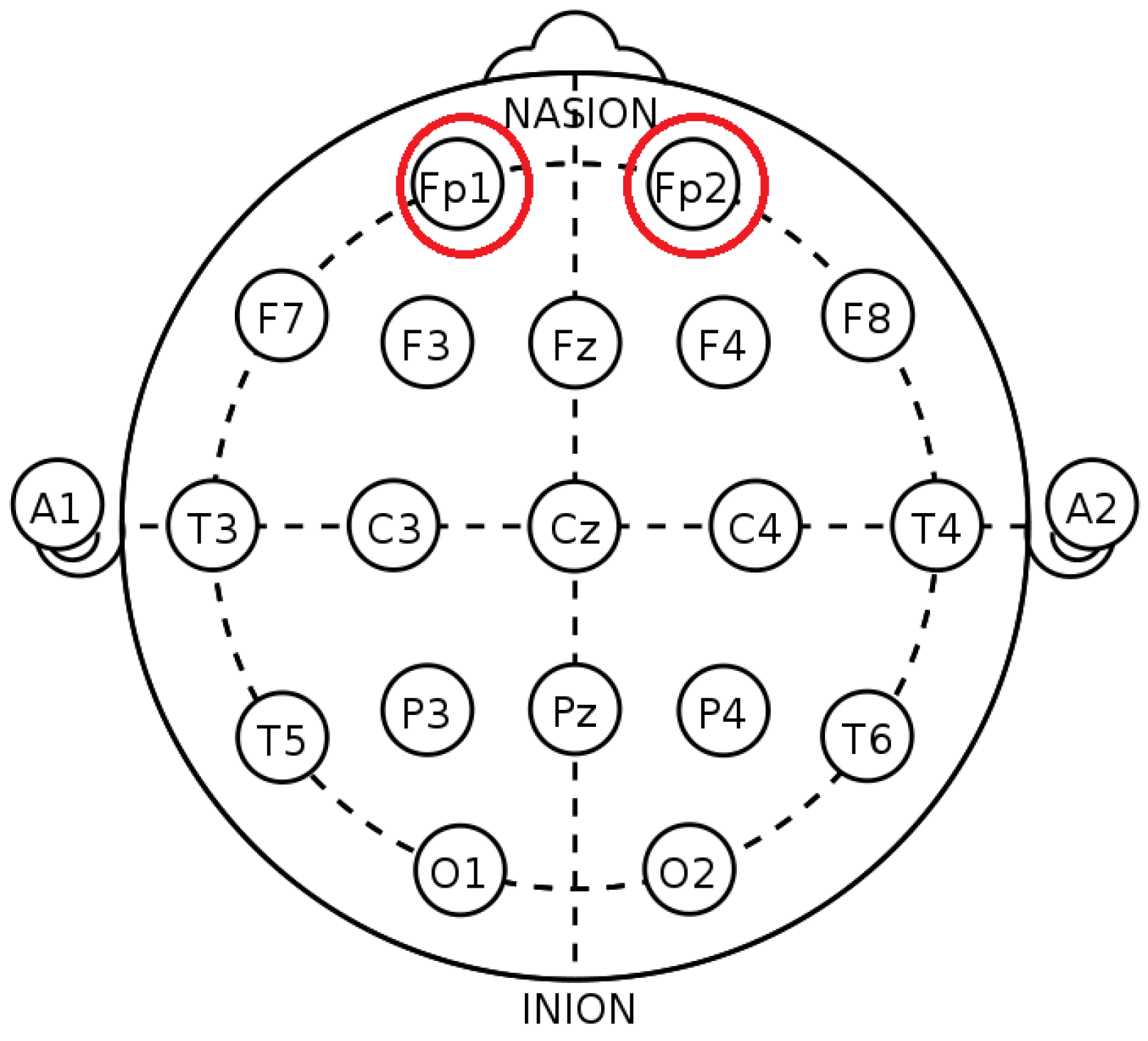
The used EEG device has a headband to attach two sensors to the FP1 and FP2 positions in the 10–20 system [27], as shown in Figure 1. Note that higher-resolution system is also widely used [27]. The device comes with a software tool to combine the recorded signal together with a time-frequency (T/F) transformation; therefore we use the transformed data in the experiments. As the EEG device is a low-price product, its signal is likely interfered by artifacts such as the eye blinking, and it is unknown whether the artifacts are removed by the accompanying software tool or not. To avoid this interference, the test subjects are asked to close their eyes during the signal recording phase.
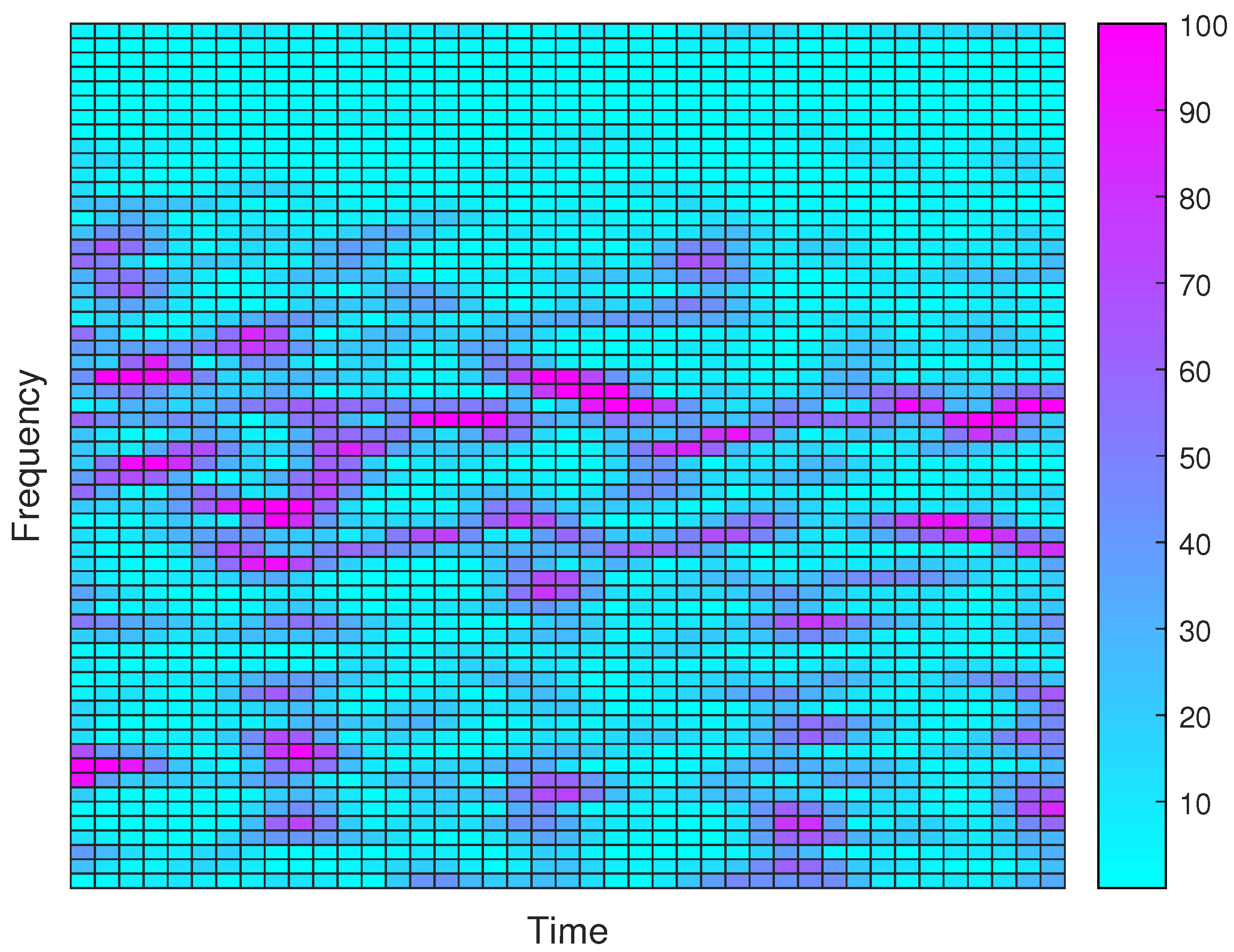
In our experiments, the recording has a duration of 10 s and a frequency range from 0 to 64 Hz. By using the time-to-frequency transformation module in the accompanying software, the collected EEG data contains energy values with a time resolution of 0.125 s and a frequency resolution of 0.25 Hz. Therefore, the obtained data in one recording can also be plotted as a spectrogram. Figure 2 shows the spectrogram of a portion of a recording from a subject in the relaxation state. In the figure, the grid on the bottom left corner has a frequency band from 4 Hz to 4.25 Hz at time 5 to 5.125 s. Its energy value is between 0 and 20 (based on the color bar). It is observed that most time-frequency grids have very small energy values, with only a few grids with large values. Actually, the energy values of this recording have a maximum of 367, a minimum of 0, a mean of 5.01, and a standard deviation of 13.56.
3.3. Feature Extraction
In conducting the experiments, the test subjects are asked to relax without concentration for 5 s. The recorded EEG data in this portion is served as the baseline. Then, the subject is either asked to recite a number backwards or just to relax (mentioned in Section 3.1) for another 5 s. Therefore, one EEG piece has a duration of 10 s. The EEG data corresponding to the sixth to eighth seconds (a duration 3 s) are used for classification. For each subject, 40 pieces of EEG signals are recorded, where 20 of them are in concentration state and the other 20 in relaxed state.
During the experiments, 70% of the collected EEG recordings are used for training, and the other 30% for testing. The training and testing procedure is repeated 40 times (trials), and the averaged performance is reported. The training and testing recordings are randomly chosen in every trial of the experiments. However, to maintain a fair comparison, the selected training and testing pieces are used for all methods examined in one trial.
As the transformed energy data are used, the data have values per second per Hertz. As the beta band has a bandwidth of 16 Hz, the total number of energy data for 3 s is . This number is too large to train classifiers. Thus, we need to reduce the dimensionality of the energy data. In our case, we simply use the average energy, although more complicated methods are also available [1]. Let the energy data of the chosen part in an EEG piece be denoted as , where n is the time index and k is the frequency index. We use the following average as basis for computing features:
where is one feature value used in the experiments with time index m (unit: second) and frequency index l (unit: Hz). We use different energy band ranges and bandwidths for different types of features, detailed below:
- (i)
- All band average energy (All band energy). In this type of feature, the total energy per second is calculated for each band (theta, alpha, beta_1, beta_2, and gamma). For beta band, we sum up all values for l from 13 to 20 in Equation (1) to form beta_1, and from 21 to 28 to form beta_2. Thus, the feature dimension to represent one EEG piece has values, i.e., 3 s with 5 bands per second.
- (ii)
- Beta band with different frequency resolution ( only). It is known that when a person is in concentration, the beta band has much stronger energy. Thus, we use this band to classify mental states. Features in this category are averaged energy of beta band in 1, 2, or 4 Hz bandwidth. As the beta band is from 13 to 28 Hz, a bandwidth of 1 Hz produces a feature of 3 × 16 = 48 dimensions for one piece of EEG signal.
- (iii)
- Beta band plus a portion of alpha band (). Similar to (ii), but the frequency range is from 9 to 28 Hz. Although it is given in the literature that higher energy appears in beta band when the subject is in the concentration mental state, different persons may have different frequency ranges in the beta band. In fact, the frequency ranges of the bands are somewhat arbitrary. As pointed out in Wikipedia on EEG [2]:Unfortunately there is no agreement in standard reference works on what these (band) ranges should be—values for the upper end of alpha and lower end of beta include 12, 13, 14 and 15 (Hz).Considering this situation, we have a strong reason to also examine energy from other bands.
- (iv)
- Beta band plus a portion of alpha and gamma band (). Similar to (ii), but the frequency range is from 9 to 43 Hz.
3.4. Used Classifiers
In the experiments, the classifiers are support vector machines (SVM), obtained from [29], and multi-layer feedforward neural network (BPNN) trained with the back propagation algorithm. SVM has been extensively used in many classification problems. Previously, Liu et al. reported that good accuracy (more than 76%) was obtained by using SVM to classify two mental states based on EEG [7]. Therefore, we also choose SVM as a classifier. To use SVM, one needs to determine many parameters. One key parameter is the kernel type, where a widely used one is the RBF (radical basis function) kernel. In the experiments, we also use this type of kernel. To use the RBF kernel, we need to provide the value of gamma. In many cases, this parameter is obtained through an extensive search. In our case, after some trials, we set this parameter to 8. In addition, we set the cost parameter to 32.
We also use the BPNN as a classifier because it is also used for EEG classification in the literature [30,31]. One reason to examine both classifiers is to observe whether one subject has good accuracy by using one classifier, but poor accuracy by using the other one. The used BPNN is a three-layer fully connected network. The number of hidden neurons is set to 10, although the classification accuracy remains almost the same from 5 to 50 hidden neurons. The performance criterion is the mean squared error. As the accuracy of the BPNN is not as good as that of the SVM, unless necessary, we only report the accuracy results based on SVM.
Recently, the convolutional neural networks (CNN) have been demonstrated to outperform traditional classifiers such as SVM in EEG classifications [32]. When used with 1D convolutional layers, the network is capable of extracting features directly from the time-domain signal. In our case, unfortunately, we did not have sufficient information to retrieve the time-domain signals. Therefore, we used the time-frequency energy values computed by the accompanying software, as described in Section 3.2. Still, it is possible to use the spectrogram as the inputs to a 2D CNN, as widely used in the vocal detection [33] problems. Actually, we have tried this idea before, but the performance was poor due to the small number of training samples (28 training samples per subject). We were suggested by the anonymous reviewer that we could use the transfer learning approach [34] to overcome the problem of small training sets. We will investigate this approach in our future work.
4. Experiments and Results
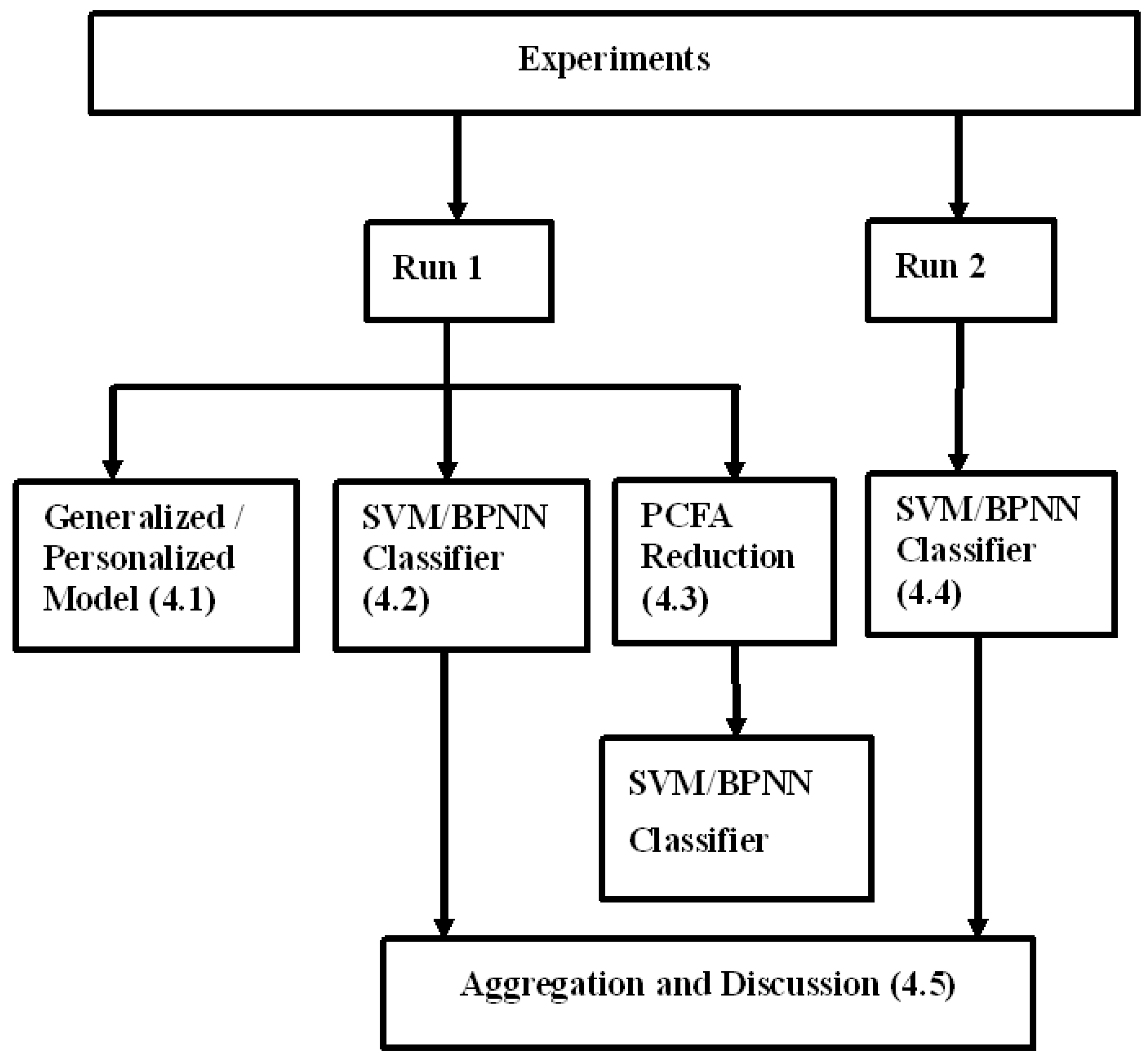
We conducted several experiments to evaluate the accuracy of the proposed approach, as shown in Figure 3. In the experiments, we have two groups (runs) of subjects. The first experiment checks if an individualized SVM model is better than a generic model with subjects in run 1 (Section 4.1). The second experiment checks which type of features described in Section 3.3 is better for both types of classifiers (Section 4.2). The third experiment examines if the dimensionality reduction technique improves the classification accuracy (Section 4.3). To check if the experiments are reproducible, we repeat the above experiments with patients in run 2 (Section 4.4). Finally, we aggregate the results in both runs with some discussions in Section 4.5.
4.1. Generic Model vs. Individualized Model
In the first experiment, the generic SVM model is trained by using the EEG pieces from all subjects, and the model is used to classify all testing EEG pieces. For the individualized SVM mode case, EEG signals from each subject is independently used to train a personalized SVM model for testing. As the brain–computer interface is typically used by one or a small group of users, it is a reasonable assumption that we can train the classifier and pick the features to fit the need of each individual user. The idea of training individual model is also used in [11].
For the first experiment, we use the features “All band energy” mentioned in Section 3.3. The accuracy is shown in Table 1. Note that the “accuracy” given in the table refers to the ratio of correctly classified items in both mental states to the total test items. From the results, we know that using individualized model improves the classification accuracy significantly. In a sense, the experimental results indicate that using individualized models for each subject is a better approach for this particular classification problem.
4.2. Features with Different Band Ranges and Different Bandwidths
To further examine which feature type has higher accuracy, we conduct the second experiment. In this experiment, the SVM models are individually trained and tested with different kinds of features, particularly feature type (ii) to (iv) given in Section 3.3. The purpose of this experiment is to know the variation of accuracy versus the used frequency range and frequency resolution.
The experimental results for this experiment using SVM are given in Table 2. To better understand the performance differences between SVM and BPNN classifiers, we also give the BPNN accuracy in Table 3. In the tables, the mean correct rates for both classes are given. In the following, we consider the concentration state as the positive state, and the relaxation state as the negative state, then the mean correct rate of the concentration state is the same as the sensitivity (true positive rate, TPR), and that of the relaxation state is the same as the specificity (true negative rate, TNR) in the literature [35]. In our case, is calculated by , where is the corrected identified positive samples and P is the total positive samples. Similarly, , where is the corrected identified negative samples and N is the total negative samples. Since we know , P, , and N, we can compute and . In addition, it can be easily shown that the false positive rate (FPR) is , and the false negative rate (FNR) is [35]. To save space, these numbers are omitted. In the table, the F1 score is computed as
where stands for true positive, false positive, and false negative.
From Table 2 and Table 3, we observe that SVM offers much higher accuracy. For SVM classifier, features derived from , BW = 2 Hz are slightly better than others in terms of average accuracy. For only and features, BW = 2 Hz has higher accuracy, and the accuracy decreases by either BW increasing or decreasing. On the other hand, the accuracy increases when BW increases for the case of features. When observing Table 3, we notice that the average accuracy tends to increase with the increase of bandwidth with the BPNN classifier. Thus, it is inconclusive if increasing BW will improve the accuracy. We will discuss this problem again in Section 4.6.
It is worth mentioning that Maskeliunas et al. [11] also used a Neurosky device to classify the mental states into attention and meditation states. They also used individualized features for each subject. However, their accuracy was around 25%. The main difference between theirs and ours lies in different features and classifiers used. Thus, we believe that although EEG devices affect the overall accuracy a lot (as observed by Maskeliunas et al.); there is still room for improvement with better algorithms.
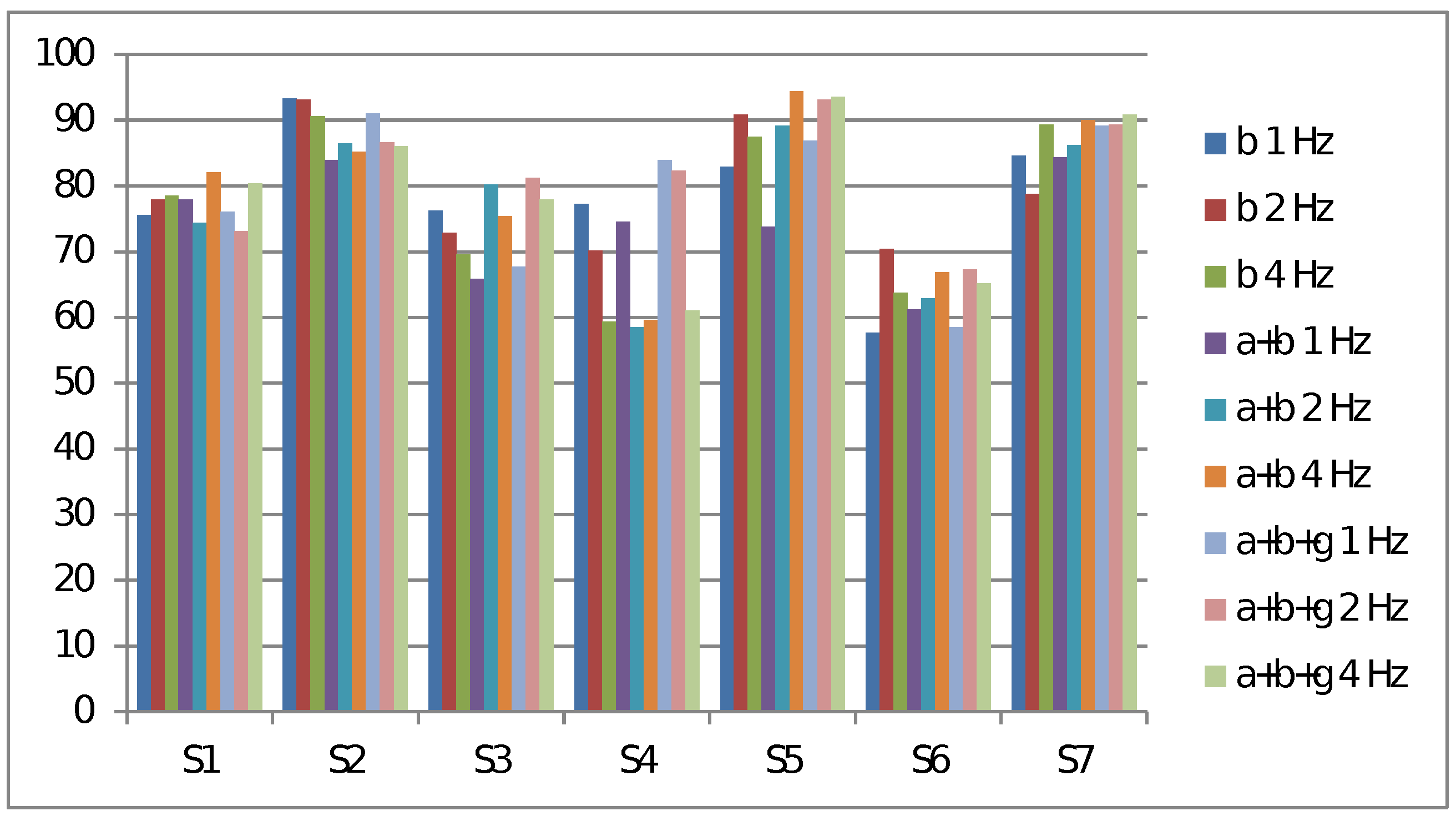
To have a better understanding about the accuracy of each individual subject with respect to each type of feature, we provide the accuracy of individual subject in Figure 4. It is observed that some subjects seem to have higher accuracy by using band only than using more bands. We will discuss the influences of classifiers on the selection of energy band ranges in Section 4.6.
4.3. Dimensionality Reduction by Factor Analysis
Previously, Morabito et al. used a stacked auto-encoder as a nonlinear method to reduce the dimensionality of the EEG features, and good results were obtained [17]. Therefore, we would also like to investigate if a dimensionality reduction technique is useful. Considering that the classification model is individually trained, we also want to reduce the dimensionality individually for each subject. As the number of training pieces per subject is small (only 28), using the auto-encoder could easily result in over-fitting. Thus, we need to use conventional methods. Previously, we have studied the use of PCA (principal component analysis) for reducing the dimensionality of spectral-temporal objects [36], and the results were promising. Later on, we also repeated the experiments by using factor analysis (FA) [36], and found that FA was more robust to distorted objects. So, we would like to investigate if FA is useful in the present case. Please note that the FA method presented is actually PCFA (principal component factor analysis). This approach is generally similar to that of the FA. The only difference is the computation of the matrix for reduction, i.e., Equation (6). As the FA approach used here is an extension of the PCA approach [36], we omit the use of the PCA in this subsection to save space.
In this experiment, the chosen full-resolution features are -only features with bandwidth of 1 Hz. For optimal performance, the FA procedure is independently carried out for each subject in one (concentration or relaxation) state. To apply FA for reduction, we use the following procedure.
- Letwhere one is a column vector formed by in one-second a duration as its elements. Therefore, contains to from a particular EEG piece. As there are 14 training pieces per subject per state, we have 14 × 3 = 42 vectors total.
- Compute the covariance matrix aswhere T denotes matrix transpose.
- Compute the eigenvalues and the associated eigenvectors for . Denote the largest p eigenvalues as with the corresponding eigenvectors , …, . In the simulation, we use p = 8, 6, or 4 for dimension reduction rates. Basically, p is the number of values remained after FA in one second. Note that full resolution has p = 16.
- Construct the loading matrix by
- The dimension-reduced features are obtained aswhere is either a training or a testing vector arranged in a form similar to that in Equation (3). As one testing EEG piece has a duration of 3 s, three vectors are concatenated as a feature vector for training or testing.
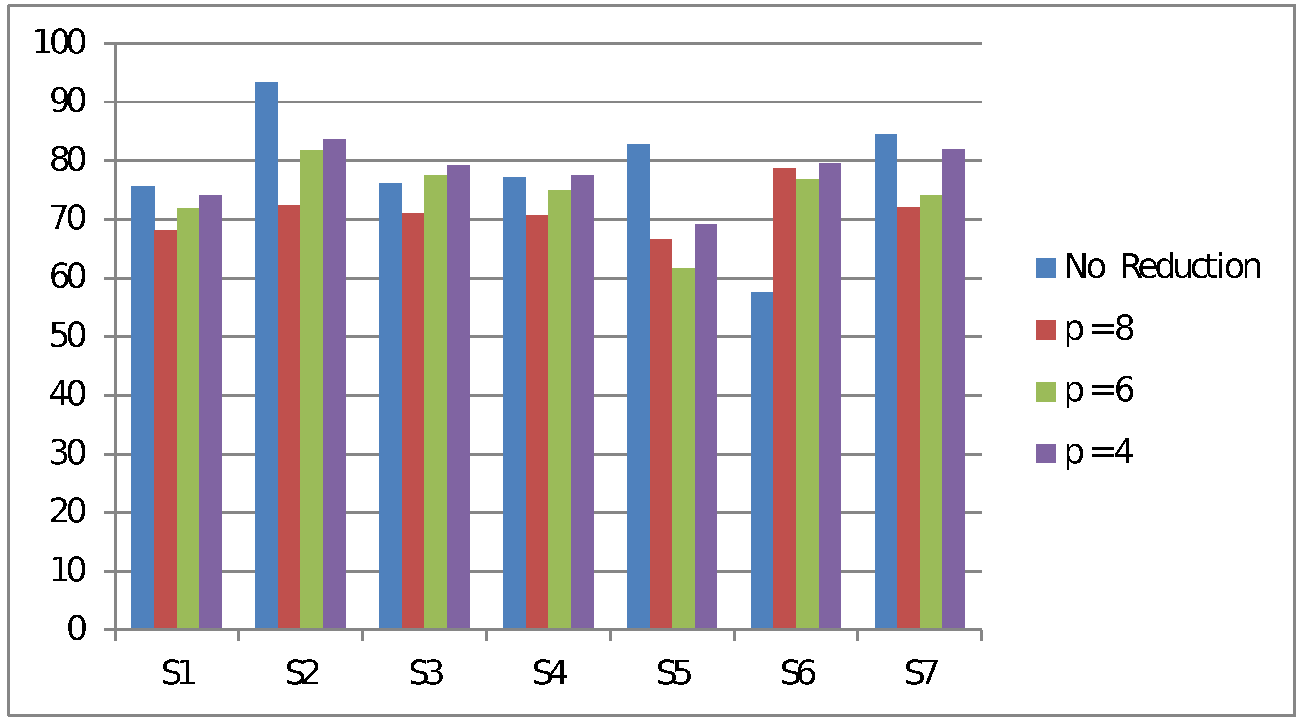
The experimental results are given in Figure 5. The results show that some subjects have lower accuracy after FA reduction, whereas some have higher accuracy, especially subject 6. Note that in the p = 8 case, one second of EEG signal produces 8 values after FA reduction, so a feature has a dimension of . The same feature dimension is obtained in the case of only with BW = 2 Hz. Similarly, p = 4 has the same feature dimension as the only, BW = 4 Hz case. When comparing FA with and only with BW = 4 Hz cases, we find that the average accuracy of the FA approach is slightly higher (77.9% vs. 77.0%). However, the performance difference is not sufficiently large to claim that FA is a better method. Nevertheless, we find that the standard deviation of the FA approach is much lower (4.9% vs. 12.9%). So, the accuracy variation among subjects is reduced. To this end, it may be worth conducting further research to see if any particular dimensionality reduction technique works better for the EEG signal in terms of minimizing the standard deviation.
4.4. Reproducible Test
As our previous experiment has only seven subjects, we are not very confident that the results we obtained can be reproduced or not. To this end, we repeat experiments two and three (in Section 4.2 and Section 4.3) with 10 different subjects. The experimental procedure remains the same, so the procedure is omitted here.
The results for experiment two are given in Table 4. The experimental results show some degree of consistency with our previous experiment, such as , 1 Hz has lower accuracy. However, in contrast to our previous experiment, the results here show that wider bandwidth (BW = 4 Hz) yields higher average accuracy than narrower ones. Furthermore, note that the average accuracy is higher than previous one. As to the BPNN classifier, the average accuracy is still lower than that of SVM, but the difference is much smaller, only about 2 to 3%.
One thing worth mentioning is that the standard deviations in Table 4 are higher than those we see in Table 2. When examining the accuracy of individual subjects, we find that several subjects have very high accuracy (higher than 90%), but some have relatively low accuracy (around 60%), and, again, the accuracy varies with different types of features. Thus, the situation we observe in Figure 4 is not a single incidence, but a general case. To save space, the accuracy plot is omitted here.
We also conducted FA experiment (Section 4.3) for these new subjects. The results show that the accuracy with FA reduction is not as good as that of the only, BW = 4 Hz (80.2% vs. 87.7%). However, we again notice the advantage of lower standard deviation in the FA approach (6.4% vs. 11.1%). Thus, the advantage of lower standard deviation is consistent to that in Section 4.3.
4.5. Discussions
In Section 4.2, we are unsure whether wider bandwidth leads to higher average accuracy. As we now have more test subjects, we then aggregate the accuracy of all test subjects in the following analysis. Because we use two classifiers (SVM and BPNN) in our previous experiments, we can perform cross comparison to observe the influences of the classifiers. Table 5 summarizes the accuracy under various conditions. We observe that, in most cases, average accuracy has the tendency to increase if the bandwidth increases. As the experimental results of FA in Section 4.3 also show that a certain degree of dimensionality reduction is beneficiary for high-dimensional EEG features, it seems safe to say that wider bandwidth tends to improve average accuracy with different energy band ranges.
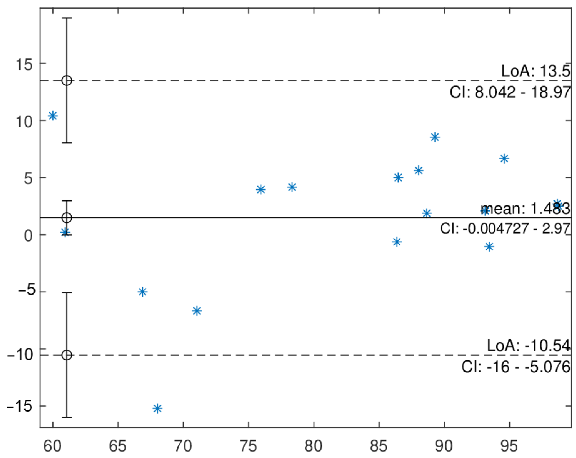
To visualize the accuracy differences between these two classifiers, we also use the Bland–Altman plot [37] for subjects in the + + , 4 Hz setting, as shown in Figure 6. The figure shows that the SVM has a higher average accuracy than the BPNN by about 1.5% (shown as the mean line). In addition, most subjects have higher accuracy by using the SVM classifier (points above zero in the vertical direction), and only one subject strongly favors the BPNN classifier. Overall, we confirm that the SVM, in general, is better in this experiment.
Previously, we mention that each subject may need different energy band ranges to yield higher accuracy. We now investigate whether this situation is due to the behavior of the classifier. In this comparison, we only consider which band range yields higher accuracy for a subject, but not the bandwidth. That is, if , 1 Hz is the best type of feature for one subject using SVM, and , 4 Hz using BPNN, we say that both are consistent. To avoid BCI illiteracy subjects affecting the comparison, only subjects with a highest accuracy (using SVM) greater than 85% are chosen in the comparison. The results are shown in Table 6. The results show that the consistency rate is 50%, not a particularly high rate. Therefore, we know that the chosen classifier has some influences on the selection of energy band range. With this understanding, we suggest using band range of , as it yields satisfactory accuracy for both types of classifiers.
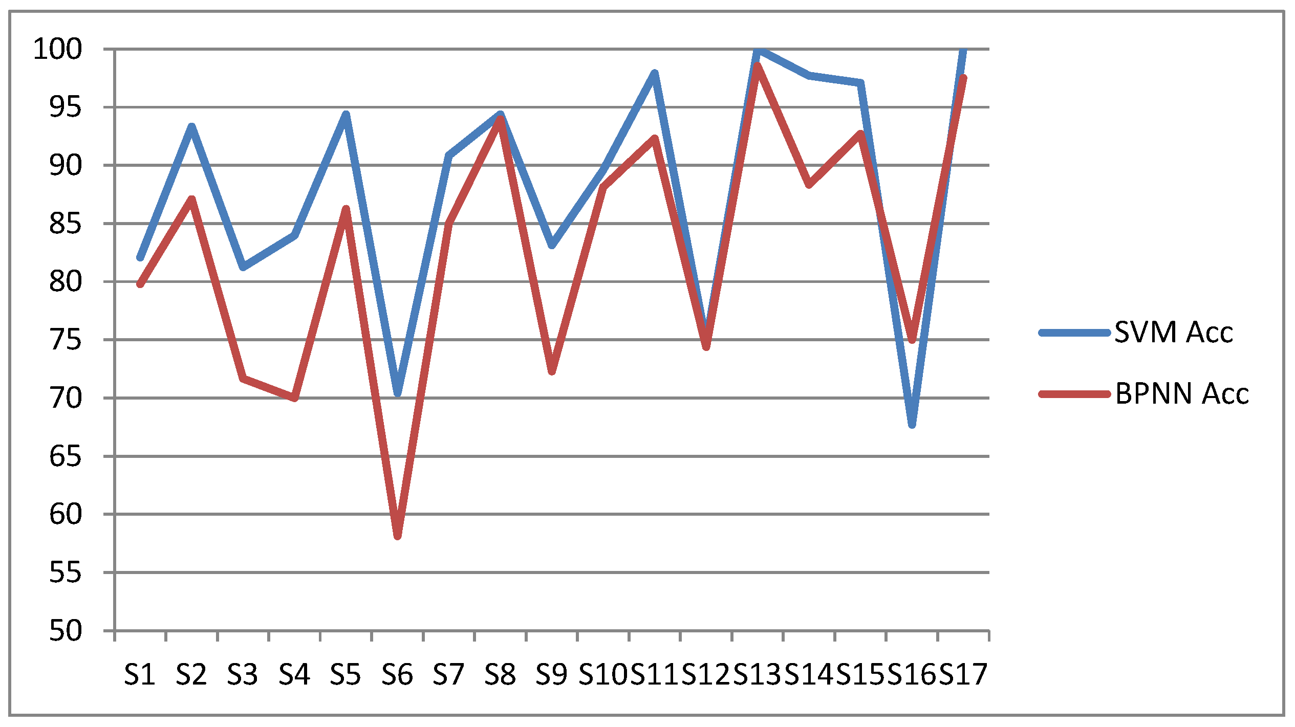
We know that individual variability plays an important role in the EEG classification problem. To see if subjects with low/high accuracy in one classifier also yield low/high accuracy in another one, we plot the highest accuracy for each individual under different types of features in Figure 7. The plot shows that both classifiers have high consistency. Thus, if the accuracy of a subject is particularly low, the problem may not be the type of used classifier. Instead, it is more likely that the subject is BCI illiteracy.
4.6. Limitations of the Study
Although the experimental results are promising, the proposed approach, nevertheless, has the following limitations.
- The subjects are clear-headed. During the experiments, we observed that a subject could not concentrate if he/she was sleepy. Therefore, it is important to check the subject’s drowsiness before conducting the experiments.
- The subjects are limited to a small group with a uniform background. Currently, the experiments were conducted with subjects aged in their 20 s with college degrees in one geographic area. Therefore, subjects with different age groups, different educational levels, and different areas will be needed in the future work.
- The proposed features are in the frequency-domain with a short period of time. Recall that the features we used represent only one channel with a duration of 3 s. However, public datasets such as DEAP (Database for Emotion Analysis using Physiological Signals) [38] have multiple channels with much longer recording time. For example, in the DEAP dataset, each EEG recording has 32 channels with a recording duration of 1 min. To apply the features presented in this paper, we need to choose one appropriate channel among the 32 channels and one particular 3-s segment from the one-minute recording. Certainly, this work is not trivial. For this type of dataset, it might be easier to use a 1D CNN classifier to extract features directly from the time-domain signal.
5. Conclusions
This paper studies the accuracy of classifying relaxed and concentrated mental states. The concentration mental state is invoked by silently reciting a five-digit number backwards. In the experiments, the training and testing recordings are from different files to reflect a more realistic situation. The experimental results show that when averaging over all 17 test subjects with , 4 Hz features, the classification accuracy can achieve 80% or higher if using individually trained models. When comparing the results from SVM and BPNN, wider bandwidth tends to improve the accuracy in most cases. On the other hand, whether a particular energy band range is better, in a certain degree, is affected by the used classifier. Even so, we recommend using features of , 4 Hz, as they produce satisfactory accuracy in the experiments for both classifiers. In addition, we find that using the FA approach can reduce the variance of accuracy. Therefore, other types of reduction technique deserve further study. Overall, we demonstrate that it is plausible to distinguish between concentrated and relaxed mental states even with the use of a cheap EEG device. In the future, we plan to examine whether the proposed feature selection mechanism is appropriate for existing EEG datasets. In addition, we also plan to study the use of CNN classifiers to classify the dataset presented in this paper to evaluate the advantages of the deep learning approach.
Funding
This research received no external funding.
Informed Consent Statement
Informed consent was obtained from all subjects involved in the study.
Data Availability Statement
The data presented in this study are available at https://github.com/NTUT-LabASPL/EEG, accessed on 10 April 2021.
Acknowledgments
The author would like to thank Cheng-Ying Sung, Yu-Cheng Wu, and Fan-Hao-Chi Fang for data collection and conducting preliminary experiments.
Conflicts of Interest
The author declares no conflict of interest.
References
- Akbar, I.A.; Igasaki, T. Drowsiness Estimation Using Electroencephalogram and Recurrent Support Vector Regression. Information 2019, 10, 217. [Google Scholar] [CrossRef] [Green Version]
- Available online: https://en.wikipedia.org/wiki/Electroencephalography (accessed on 10 April 2021).
- Lin, Y.P.; Wang, C.H.; Jung, T.P.; Wu, T.L.; Jeng, S.K.; Duann, J.R.; Chen, J.H. EEG-based emotion recognition in music listening. IEEE Trans. Biomed. Eng. 2010, 57, 1798–1806. [Google Scholar] [PubMed]
- Koelstra, S.; Muhl, C.; Soleymani, M.; Lee, J.; Yazdani, A.; Ebrahimi, T.; Pun, T.; Nijholt, A.; Patras, I. DEAP: A database for emotion analysis; using physiological signals. IEEE Trans. Affect. Comput. 2012, 3, 18–31. [Google Scholar] [CrossRef] [Green Version]
- Patsis, G.; Sahli, H.; Verhelst, W.; De Troyer, O. Evaluation of attention levels in a tetris game using a brain computer interface. Lect. Notes Comput. Sci. 2013, 7899, 127–138. [Google Scholar]
- Vyšata, O.; Schätz, M.; Kopal, J.; Burian, J.; Procházka, A.; Jiří, K.; Hort, J.; Vališ, M. Non-Linear EEG measures in meditation. J. Biomed. Sci. Eng. 2014, 7, 731–738. [Google Scholar] [CrossRef] [Green Version]
- Liu, N.-H.; Chiang, C.-Y.; Chu, H.-C. Recognizing the degree of human attention using EEG signals from mobile sensors. Sensors 2013, 13, 10273–10286. [Google Scholar] [CrossRef] [PubMed]
- Li, Y.; Li, X.; Ratcliffe, M.; Liu, L.; Qi, Y.; Liu, Q. A real-time EEG-based BCI system for attention recognition in ubiquitous environment. In Proceedings of the 2011 International Workshop on Ubiquitous Affective Awareness and Intelligent Interaction (UAAII’11), Beijing, China, 18 September 2011; pp. 33–40. [Google Scholar]
- Liang, Z.; Liu, H.; Mak, J.N. Detection of media enjoyment using single-channel EEG. In Proceedings of the 2016 IEEE Biomedical Circuits and Systems Conference (BioCAS), Shanghai, China, 17–19 October 2016; pp. 516–519. [Google Scholar]
- Katona, J.; Ujbanyi, T.; Sziladi, G.; Kovari, A. Speed control of Festo Robotino mobile robot using NeuroSky MindWave EEG headset based brain–computer interface. In Proceedings of the 2016 7th IEEE International Conference on Cognitive Infocommunications (CogInfoCom), Wroclaw, Poland, 16–18 October 2016; pp. 251–256. [Google Scholar]
- Maskeliunas, R.; Damasevicius, R.; Martisius, I.; Vasiljevas, M. Consumer-grade EEG devices: Are they usable for control tasks? PeerJ 2016, 4, e1746. [Google Scholar] [CrossRef] [PubMed]
- Morshad, S.; Mazumder, M.R.; Ahmed, F. Analysis of Brain Wave Data Using Neurosky Mindwave Mobile II. In Proceedings of the International Conference on Computing Advancements; Association for Computing Machinery: New York, NY, USA, 2020; pp. 1–4. [Google Scholar]
- Jiang, L.; Guan, C.; Zhang, H.; Wang, C.; Jiang, B. Brain computer interface based 3D game for attention training and rehabilitation. In Proceedings of the 6th IEEE Conference on Industrial Electronics and Applications, Beijing, China, 21–23 June 2011; pp. 124–127. [Google Scholar]
- Rebolledo-Mendez, G.; Dunwell, I.; Martínez-Mirón, E.A.; Vargas-Cerdán, M.D.; De Freitas, S.; Liarokapis, F.; García-Gaona, A.R. Assessing NeuroSky’s usability to detect attention levels in an assessment exercise. Lect. Notes Comput. Sci. 2009, 5610, 149–158. [Google Scholar]
- Hamadicharef, B.; Zhang, H.; Guan, C.; Wang, C.; Phua, K.S.; Tee, K.P.; Ang, K.K. Learning EEG-based spectral-spatial patterns for attention level measurement. In Proceedings of the 2009 IEEE International Symposium on Circuits and Systems, Taipei, Taiwan, 24–27 May 2009; pp. 1465–1468. [Google Scholar]
- Kahneman, D. Thinking, Fast and Slow; Farrar, Straus and Giroux: New York, NY, USA, 2011. [Google Scholar]
- Morabito, F.C.; Campolo, M.; Mammone, N.; Versaci, M.; Franceschetti, S.; Tagliavini, F.; Sofia, V.; Fatuzzo, D.; Gambardella, A.; Labate, A. Deep learning representation from electroencephalography of Early-Stage Creutzfeldt-Jakob disease and features for differentiation from rapidly progressive dementia. Int. J. Neural Syst. 2017, 27, 1–15. [Google Scholar] [CrossRef]
- Ahn, M.; Cho, H.; Ahn, S.; Jun, S.C. High Theta and Low Alpha Powers May Be Indicative of BCI-Illiteracy in Motor Imagery. PLoS ONE 2013, 8, e80886. [Google Scholar] [CrossRef] [PubMed] [Green Version]
- Blankertz, B.; Sannelli, C.; Halder, S.; Hammer, E.M.; Kübler, A.; Müller, K.R.; Curio, G.; Dickhaus, T. Neurophysiological predictor of SMR-based BCI performance. Neuroimage 2010, 51, 1303–1309. [Google Scholar] [CrossRef] [PubMed] [Green Version]
- Vuckovic, A. Motor imagery questionnaire as a method to detect BCI illiteracy. In Proceedings of the 2010 3rd International Symposium on Applied Sciences in Biomedical and Communication Technologies (ISABEL), Rome, Italy, 7–10 November 2010; pp. 1–5. [Google Scholar]
- Ahn, M.; Ahn, S.; Hong, J.H.; Cho, H.; Kim, K.; Kim, B.S.; Chang, J.W.; Jun, S.C. Gamma band activity associated with BCI performance: Simultaneous MEG/EEG study. Front. Hum. Neurosci. 2013, 7. [Google Scholar] [CrossRef] [PubMed] [Green Version]
- Ali, F.; El-Sappagh, S.; Islam, S.R.; Ali, A.; Attique, M.; Imran, M.; Kwak, K.S. An intelligent healthcare monitoring framework using wearable sensors and social networking data. Future Gener. Comput. Syst. 2021, 114, 23–43. [Google Scholar] [CrossRef]
- Sarkar, S.K.; Roy, S.; Alsentzer, E.; McDermott, M.B.A.; Falck, F.; Bica, I.; Adams, G.; Pfohl, S.; Hyland, S.L. Machine Learning for Health (ML4H) 2020: Advancing Healthcare for All. Proc. Mach. Learn. Res. 2020, 136, 1–11. Available online: http://proceedings.mlr.press/v136/sarkar20a.html (accessed on 10 April 2021).
- Hyland, S.L.; Faltys, M.; Hüser, M.; Lyu, X.; Gumbsch, T.; Esteban, C.; Bock, C.; Horn, M.; Moor, M.; Rieck, B. Early prediction of circulatory failure in the intensive care unit using machine learning. Nat. Med. 2020, 26, 364–373. [Google Scholar] [CrossRef] [PubMed]
- Ali, F.; El-Sappagh, S.; Islam, S.R.; Kwak, D.; Ali, A.; Imran, M.; Kwak, K.S. A smart healthcare monitoring system for heart disease prediction based on ensemble deep learning and feature fusion. Inf. Fusion 2020, 63, 208–222. [Google Scholar] [CrossRef]
- Available online: https://en.wikipedia.org/wiki/N-back (accessed on 10 April 2021).
- Available online: https://en.wikipedia.org/wiki/10%E2%80%9320_system_(EEG) (accessed on 10 April 2021).
- Public Domain. Available online: https://en.wikipedia.org/wiki/10%E2%80%9320_system_(EEG)#/media/File:21_electrodes_of_International_10-20_system_for_EEG.svg (accessed on 10 April 2021).
- LIBSVM—A Library for Support Vector Machines. Available online: https://www.csie.ntu.edu.tw/~cjlin/libsvm/ (accessed on 10 April 2021).
- Ghosh, R.; Sinha, N.; Singh, N. Emotion recognition from EEG signals using back propagation neural network. In Proceedings of the 2019 2nd International Conference on Innovations in Electronics, Signal Processing and Communication (IESC), Shillong, India, 1–2 March 2019; pp. 188–191. [Google Scholar]
- Kshirsagar, P.; Akojwar, S. Optimization of BPNN parameters using PSO for EEG signals. In Proceedings of the International Conference on Communication and Signal Processing 2016 (ICCASP 2016); Atlantis Press: Dordrecht, The Netherlands, 2016; pp. 384–393. [Google Scholar]
- Cheah, K.H.; Nisar, H.; Yap, V.V.; Lee, C.Y. Convolutional neural networks for classification of music-listening EEG: Comparing 1D convolutional kernels with 2D kernels and cerebral laterality of musical influence. Neural Comput. Appl. 2020, 32, 8867. [Google Scholar] [CrossRef]
- You, S.D.; Liu, C.H.; Lin, J.W. Improvement of Vocal Detection Accuracy Using Convolutional Neural Networks. KSII Trans. Internet Inf. Syst. 2021, 15, 729–748. [Google Scholar] [CrossRef]
- Available online: https://machinelearningmastery.com/transfer-learning-for-deep-learning/ (accessed on 10 April 2021).
- Available online: https://en.wikipedia.org/wiki/Sensitivity_and_specificity (accessed on 10 April 2021).
- You, S.D.; Hung, M. Comparative Study of Dimensionality Reduction Techniques for Spectral-Temporal Data. Information 2021, 12, 1. [Google Scholar] [CrossRef]
- Giavarina, D. Understanding Bland Altman analysis. Biochem. Med. 2015, 25, 141. [Google Scholar] [CrossRef] [PubMed] [Green Version]
- DEAP Database. Available online: http://www.eecs.qmul.ac.uk/mmv/datasets/deap/ (accessed on 10 April 2021).
Figure 1.
The attached sensors in the 10–20 system [28].
Figure 1.
The attached sensors in the 10–20 system [28].

Figure 2.
A portion of a recording displayed as a spectrogram. Note that energy values greater than 100 are limited to 100.
Figure 2.
A portion of a recording displayed as a spectrogram. Note that energy values greater than 100 are limited to 100.

Figure 3.
Framework of the experiments.

Figure 4.
Accuracy comparison for each subject with different types of features. In the legends, a means , b means , and g means .
Figure 4.
Accuracy comparison for each subject with different types of features. In the legends, a means , b means , and g means .

Figure 5.
Accuracy comparison by various levels of dimensionality reduction.

Figure 6.
The Bland–Altman plot for + + , 4 Hz case. The LOA means limits of agreement and CI is the confidence interval.
Figure 6.
The Bland–Altman plot for + + , 4 Hz case. The LOA means limits of agreement and CI is the confidence interval.

Figure 7.
Highest accuracy for each subject with SVM or BPNN classifier. The horizontal axis is the subject index and the vertical axis is accuracy.
Figure 7.
Highest accuracy for each subject with SVM or BPNN classifier. The horizontal axis is the subject index and the vertical axis is accuracy.


Table 1.
Results for experiment I. The numbers given are percentage.
| Setting | Accuracy |
|---|---|
| All band energy with common SVM Model | 57.1% |
| All band energy with individual SVM model | 74.4% |
Table 2.
Results for experiment II using SVM. The numbers given are percentage.
| Sensitivity | Specificity | Accuracy | |||||
|---|---|---|---|---|---|---|---|
| Metric | Mean | Std. | Mean | Std. | Mean | std. | F1 Score |
| only, 1 Hz | 75.9 | 15.4 | 80.6 | 15.7 | 78.2 | 11.0 | 77.4 |
| only, 2 Hz | 76.0 | 12.7 | 82.4 | 8.6 | 79.2 | 9.4 | 78.2 |
| only, 4 Hz | 71.0 | 20.3 | 82.9 | 9.9 | 77.0 | 12.9 | 74.3 |
| + , 1 Hz | 74.3 | 23.1 | 74.8 | 25.3 | 74.5 | 8.7 | 73.3 |
| + , 2 Hz | 74.1 | 16.5 | 79.6 | 14.5 | 76.8 | 12.1 | 75.9 |
| + , 4 Hz | 74.9 | 18.4 | 83.2 | 8.4 | 79.1 | 12.5 | 77.4 |
| + + , 1 Hz | 78.3 | 20.6 | 79.8 | 22.4 | 79.0 | 12.2 | 78.1 |
| + + , 2 Hz | 79.5 | 11.1 | 84.2 | 11.6 | 81.9 | 9.1 | 81.4 |
| + + , 4 Hz | 74.5 | 18.2 | 84.1 | 8.9 | 79.3 | 12.4 | 77.4 |
Table 3.
Results for experiment II using BPNN. The numbers given are percentage.
| Sensitivity | Specificity | Accuracy | |||||
|---|---|---|---|---|---|---|---|
| Metric | Mean | Std. | Mean | Std. | Mean | std. | F1 Score |
| only, 1 Hz | 66.8 | 15.0 | 73.3 | 11.3 | 70.1 | 9.7 | 68.6 |
| only, 2 Hz | 68.2 | 13.7 | 74.8 | 14.4 | 71.5 | 11.0 | 70.4 |
| only, 4 Hz | 70.8 | 18.3 | 76.4 | 11.6 | 73.6 | 12.8 | 72.1 |
| + , 1 Hz | 66.1 | 16.4 | 72.2 | 12.9 | 69.2 | 11.0 | 67.7 |
| + , 2 Hz | 68.9 | 14.6 | 74.8 | 13.2 | 71.8 | 11.7 | 70.8 |
| + , 4 Hz | 69.5 | 16.3 | 79.3 | 12.5 | 74.4 | 12.8 | 72.7 |
| + + , 1 Hz | 67.3 | 14.3 | 74.5 | 11.7 | 70.9 | 8.0 | 69.4 |
| + + , 2 Hz | 70.8 | 14.4 | 79.3 | 13.4 | 75.1 | 10.5 | 73.7 |
| + + , 4 Hz | 69.3 | 18.2 | 80.0 | 11.9 | 74.7 | 12.6 | 72.6 |
Table 4.
Results for reproducible test. The numbers given are percentage.
| Sensitivity | Specificity | Accuracy | |||||
|---|---|---|---|---|---|---|---|
| Metric | Mean | Std. | Mean | Std. | Mean | std. | F1 Score |
| only, 1 Hz | 74.6 | 24.5 | 94.6 | 6.9 | 84.6 | 15.0 | 81.1 |
| only, 2 Hz | 82.0 | 19.2 | 88.5 | 15.3 | 85.3 | 14.9 | 84.2 |
| only, 4 Hz | 85.8 | 14.8 | 89.6 | 8.0 | 87.7 | 11.1 | 87.1 |
| + , 1 Hz | 59.6 | 30.0 | 94.0 | 7.1 | 76.8 | 17.5 | 68.5 |
| + , 2 Hz | 67.3 | 27.8 | 95.3 | 5.5 | 81.3 | 15.8 | 75.3 |
| + , 4 Hz | 79.0 | 20.6 | 87.4 | 20.0 | 83.2 | 17.3 | 81.9 |
| + + , 1 Hz | 65.1 | 28.7 | 93.7 | 7.5 | 79.4 | 17.1 | 73.1 |
| + + , 2 Hz | 75.4 | 25.9 | 94.5 | 5.8 | 85.0 | 15.2 | 81.2 |
| + + , 4 Hz | 83.8 | 18.2 | 87.5 | 15.0 | 85.6 | 15.4 | 84.9 |
Table 5.
Accuracy of aggregating both groups of subjects. The numbers given are percentage.
| SVM | BPNN | |||||||
|---|---|---|---|---|---|---|---|---|
| Metric | Acc | Sens. | Spec. | F1 Score | Acc | Sens. | Spec. | F1 Score |
| only, 1 Hz | 82.0 | 75.1 | 88.8 | 80.9 | 76.2 | 78.1 | 74.3 | 78.0 |
| only, 2 Hz | 82.8 | 79.5 | 86.0 | 83.4 | 77.5 | 78.7 | 76.4 | 79.2 |
| only, 4 Hz | 83.3 | 79.7 | 86.9 | 85.4 | 80.0 | 81.1 | 78.8 | 81.4 |
| + , 1 Hz | 75.9 | 65.6 | 86.1 | 71.1 | 75.7 | 78.6 | 72.8 | 77.7 |
| + , 2 Hz | 79.4 | 70.1 | 88.8 | 77.1 | 77.9 | 79.9 | 76.0 | 79.7 |
| + , 4 Hz | 81.5 | 77.3 | 85.7 | 82.5 | 80.9 | 81.2 | 80.5 | 83.3 |
| + + , 1 Hz | 79.3 | 70.5 | 88.0 | 75.8 | 76.7 | 78.7 | 74.7 | 78.6 |
| + + , 2 Hz | 83.7 | 77.1 | 90.3 | 82.4 | 80.2 | 80.9 | 79.5 | 82.3 |
| + + , 4 Hz | 83.0 | 79.9 | 86.1 | 84.6 | 81.5 | 81.5 | 81.5 | 84.0 |
Table 6.
Energy band range yielding highest accuracy for some subjects using both classifiers. To save space, is denoted as .
Table 6.
Energy band range yielding highest accuracy for some subjects using both classifiers. To save space, is denoted as .
| Classifier | S2 | S5 | S7 | S8 | S10 | S11 | S13 | S14 | S15 | S17 |
|---|---|---|---|---|---|---|---|---|---|---|
| SVM | ||||||||||
| BPNN |
Publisher’s Note: MDPI stays neutral with regard to jurisdictional claims in published maps and institutional affiliations. |
© 2021 by the author. Licensee MDPI, Basel, Switzerland. This article is an open access article distributed under the terms and conditions of the Creative Commons Attribution (CC BY) license (https://creativecommons.org/licenses/by/4.0/).
Share and Cite
MDPI and ACS Style
You, S.D. Classification of Relaxation and Concentration Mental States with EEG. Information 2021, 12, 187. https://0-doi-org.brum.beds.ac.uk/10.3390/info12050187
AMA Style
You SD. Classification of Relaxation and Concentration Mental States with EEG. Information. 2021; 12(5):187. https://0-doi-org.brum.beds.ac.uk/10.3390/info12050187
Chicago/Turabian StyleYou, Shingchern D. 2021. "Classification of Relaxation and Concentration Mental States with EEG" Information 12, no. 5: 187. https://0-doi-org.brum.beds.ac.uk/10.3390/info12050187
Note that from the first issue of 2016, this journal uses article numbers instead of page numbers. See further details here.