On the Distributed Construction of Stable Networks in Polylogarithmic Parallel Time

Abstract

We study the class of networks, which can be created in polylogarithmic parallel time by network constructors: groups of anonymous agents that interact randomly under a uniform random scheduler with the ability to form connections between each other. Starting from an empty network, the goal is to construct a stable network that belongs to a given family. We prove that the class of trees where each node has any $k\ge 2$ children can be constructed in $O(logn)$ parallel time with high probability. We show that constructing networks that are k-regular is $\mathsf{\Omega }\left(n\right)$ time, but a minimal relaxation to $(l,k)$-regular networks, where $l=k-1$, can be constructed in polylogarithmic parallel time for any fixed k, where $k>2$. We further demonstrate that when the finite-state assumption is relaxed and k is allowed to grow with n, then $k=loglogn$ acts as a threshold above which network construction is, again, polynomial time. We use this to provide a partial characterisation of the class of polylogarithmic time network constructors.

1. Introduction

Passively dynamic networks are an important type of dynamic network in which the network dynamics are external to the algorithm and are a property of the environment in which a given system operates. Wireless sensor networks in which individual sensors are carried by autonomous entities, such as animals, or are deployed in a dynamic environment, such as the flow of a river, are examples of passively dynamic networks. In terms of modelling such systems, the network dynamics are usually assumed to be controlled by an adversary scheduler who has exclusive control over the interaction or communication sequence among the computational entities.

One line of research assumes the scheduler to be fair in the sense that it can forever conceal potentially reachable configurations of the system. This sub-type of passively dynamic networks are known as population protocols and were introduced in the seminal paper of Angluin et al. [1]. A type of fair scheduler, which is typically assumed when the running time of protocols is to be analysed, is the uniform random scheduler, which in every discrete step, selects equiprobably a pair of entities to interact from all permissible pairs of entities. Traditionally, the population protocols literature considers extremely weak entities and the goal is to reveal the computational possibilities and limitations under such a challenging interaction scheme. Recent progress has highlighted the interesting trade-offs between local space of the entities and the running time of protocols, showing, among other things that very fast running times (where fast is, here, considered to be anything growing as polylog$\left(n\right)$, n being the total number of entities in the system) can be achieved for a wide range of basic distributed tasks if the entities are equipped with as few states as polylog$\left(n\right)$. Alistarh and Gelashvili [2] also proposed the first sub-linear leader election protocol, which stabilises in $O\left({log}^{3}n\right)$ parallel time, assuming $O\left({log}^{3}n\right)$ states at each agent. Gasieniec and Stachowiak [3] designed a space optimal ($O(loglogn)$ states) leader election protocol, which stabilises in $O\left({log}^{2}n\right)$ parallel time. General characterisations, including upper and lower bounds of the trade-offs between time and space in population protocols, are provided in [4]. Doty et al. [5] showed that a state count of $O\left(n^{60}\right)$ enables fast and exact population counting.

Another line considers worst-case adversary schedulers, which may even be aware of the protocol and try to optimise against it. There, the entities are typically assumed to be powerful, such as processors of traditional distributed systems, and the only restrictions imposed on the scheduler are instantaneous or temporal connectivity restrictions, which essentially do not allow the scheduler to forever block communication between any two parts of the system. This was initiated by O’Dell and Wattenhofer [6] for the asynchronous case, and then the synchronous case was extensively studied in a series of papers by Kuhn et al. [7]. Michail et al. [8] extended this to the case of possibly disconnected dynamic networks in which connectivity is only guaranteed in a temporal sense.

The other main type of dynamic networks, with respect to who controls the changes in the network topology, are actively dynamic networks. In such networks, the algorithm is able to either implicitly change the sequence of interactions by controlling the mobility of the entities or explicitly modify the network structure by creating and destroying communication links at will. This is, for example, the subject of the area of overlay network construction [9,10,11,12]; very recently, Michail et al. introduced a fully distributed model for computation and reconfiguration in actively dynamic networks [13].

An interesting alternative family of dynamic networks rises when one considers a mixture of the passive network dynamics of the environment and the active dynamics resulting from an algorithm that can partially control the network changes or that can fix network structures that the environment is unable to affect. This is naturally motivated by molecular interactions where, for example, proteins can bind to each other, forming structures and maintaining their stability despite the dynamicity of the solution in which they reside. Michail and Spirakis [14] introduced and studied such an abstract model of distributed network construction, called the network constructors model, where the network dynamicity is the same as in population protocols but now the finite-state entities can additionally activate and deactivate pairwise connections upon their interactions. It was shown that very complex global networks can be formed stably, despite the dynamicity of the environment. Then, Michail [15] studied a geometric variant of network constructors in which the entities can only form geometrically constrained shapes in 2D or 3D space. Another interesting hybrid dynamic network model is the one by Gmyr et al. [16] in which the entities have partial control over the connections of an otherwise worst-case passively dynamic network, following the model of Kuhn et al. [7].

Our Approach

We investigate which families of networks can be stably constructed by a distributed computing system in polylogarithmic parallel time. To our knowledge, this is the first attempt made to approach this task.

Our protocols assume the existence of a leader node. A node x is a leader node if in the initial configuration, all $u\in V\backslash \left\{x\right\}$, where V is the set of all nodes, are in state $q_0$ and x is in state $s\ne q_0$.

We first study the k-children spanning tree problem, where the goal is to construct a tree where each node has, at most $k\ge 2$, children. We show that it is possible to solve this problem for any k in $O(logn)$ time with high probability. We then show that network constructors which create k-regular graphs necessarily take $\mathsf{\Omega }\left(n\right)$ time. However, with minimal relaxation to $(k,k-1)$-regular networks, the problem can be solved for any constant $k\ge 2$ in polylogarithmic time. We examine this as a special case of the $(l,k)$-Regular Network problem, where the goal is to construct a spanning network in which every node has at least $l<k$ and at most k connections, where $2<k<n$. We then transition to experimental analysis of the protocol, which not only provides evidence of the sharp contrast of the minimal relaxation but also reveals a threshold value for k, beyond which the problem reverts to polynomial time. We use this knowledge to propose a first partial characterisation of the set of polylogarithmic time network constructors. We leave providing formal bounds as an open problem.

In Section 2, we formally define the model of network constructors and the network construction problems that are considered in this work. In Section 3, we study the k-children spanning tree problem and provide the lower bound for k-regular networks. We then present a protocol for the $(l,k)$-regular network problem and our experimental analysis, culminating in partial characterisation. In Section 4, we conclude and give further research directions that are opened by our work.

2. Materials and Methods

2.1. The Model

Definition 1.

A Network Constructor (NET) is a distributed protocol defined by a 4-tuple $(Q,q_0,Q_{out},\delta )$, where Q is a finite set of node-states, $q_0\in Q$ is the initial node-state, $Q_{out}\subseteq Q$ is the set of output node-states, and $\delta :Q\times Q\times \{0,1\}\to Q\times Q\times \{0,1\}$ is the transition function.

If $\delta (a,b,c)=(a^{\prime },b^{\prime },c^{\prime })$, we call $(a,b,c)\to (a^{\prime },b^{\prime },c^{\prime })$ a transition (or rule) and we define ${\delta }_1(a,b,c)=a^{\prime },{\delta }_2(a,b,c)=b^{\prime }$, and ${\delta }_3(a,b,c)=c^{\prime }$. A transition $(a,b,c)\to (a^{\prime },b^{\prime },c^{\prime })$ is called effective if $x\ne x^{\prime }$ for at least one $x\in \{a,b,c\}$ and ineffective otherwise. When we present the transition function of a protocol, we only present the effective transitions. Additionally, we agree that the size of a protocol is the number of its states, i.e., $\left|Q\right|$.

The system consists of a population $V_I$ of n distributed processes (called nodes for the rest of this paper). In the generic case, there is an underlying interaction graph $G_I=(V_I,E_I)$ specifying the permissible interactions between the nodes. Interactions in this model are always pairwise. In this work, $G_I$ is a complete undirected interaction graph, i.e., $E_I=\{uv:u,v\in V_I \mathrm{and}u\ne v\}$, where $uv=\{u,v\}$. Initially, all nodes in $V_I$ are in the initial node-state $q_0$. A central assumption of the model is that edges have binary states. An edge in state 0 is said to be inactive while an edge in state 1 is said to be active. All edges are initially inactive. Execution of the protocol proceeds in discrete steps. In every step, a pair of nodes $uv$ from $E_I$ is selected by an adversary scheduler and these nodes interact and update their states and the state of the edge joining them, according to the transition function $\delta$.

A configuration is a mapping $C:V_I\cup E_I\to Q\cup \{0,1\}$ specifying the state of each node and each edge of the interaction graph. Let C and $C^{\prime }$ be configurations, and let $u,\upsilon$ be distinct nodes. We say that C goes to $C^{\prime }$ via encounter$e=u\upsilon$, denoted $C\stackrel{e}{\to }{C}^{\prime }$, if $(C^{\prime }\left(u\right),C^{\prime }\left(v\right),C^{\prime }\left(e\right))=\delta (C\left(u\right),C\left(v\right),C\left(e\right))$ or $(C^{\prime }\left(v\right),C^{\prime }\left(u\right),C^{\prime }\left(e\right))=\delta (C\left(v\right),C\left(u\right),C\left(e\right))$ and $C^{\prime }\left(z\right)=C\left(z\right)$, for all $z\in (V_I\backslash \{u,v\})\cup (E_I\backslash \left\{e\right\})$. We say that $C^{\prime }$ is reachable in one step from C, denoted $C\to C^{\prime }$, if $C\stackrel{e}{\to }{C}^{\prime }$ for some encounter $e\in E_I$. We say that $C^{\prime }$ is reachable from C and write $C⇝C^{\prime }$, if there is a sequence of configurations $C=C_0,C_1,\dots ,C_t=C^{\prime }$, such that $C_i\to C_{i+1}$ for all $i,0\le i<t$.

An execution is a finite or infinite sequence of configurations $C_0,C_1,C_2,\dots ,$ where $C_0$ is an initial configuration and $C_i\to C_{i+1}$, for all $i\ge 0$. A fairness condition is imposed on the adversary to ensure that the protocol makes progress. An infinite execution is fair if for every pair of configurations C and $C^{\prime }$ such that $C\to C^{\prime }$, if C occurs infinitely often in the execution then so does $C^{\prime }$. In what follows, every execution of a NET is, by definition, considered to be fair.

We define the output of a configuration C as the graph $G\left(C\right)=(V,E)$ where $V=\{u\in V_I:C\left(u\right)\in Q_{out}\}$ and $E=\{uv:u,v\in V,u\ne v,\mathrm{and}C(uv)=1\}$. In words, the output graph of a configuration consists of those nodes that are in output states and those edges between them that are active, i.e., the active subgraph induced by the nodes that are in output states. The output of an execution $C_0,C_1,\dots$ is said to stabilize (or converge) to a graph G if there exists some step $t\ge 0$ such that (abbreviated “s.t.” in several places) $G\left(C_i\right)=G$ for all $i\ge t$, i.e., from step t and onwards, the output graph remains unchanged. Every such configuration $C_i$, for $i\ge t$ is called output stable. The running time (or time to convergence) of an execution is defined as the minimum, such as t (or ∞ if no such t exists). Throughout the paper, whenever we study the running time of a NET, we assume that interactions are chosen by a uniform random scheduler, which, in every step, selects independently and uniformly at random one of the $|E_I|=n(n-1)/2$ possible interactions. In this case, the running time becomes a random variable (abbreviated “r.v.” throughout) X and our goal is to obtain bounds on the expectation $E\left[X\right]$ of X. Note that the uniform random scheduler is fair with probability 1.

In this work, “time” is treated as sequential in our analyses, i.e., a time step consists of a single interaction selected by the scheduler. Such a sequential estimate can be easily translated to some estimate of parallel time. For example, assuming that $\mathsf{\Theta }\left(n\right)$ interactions occur in parallel in every step, one could obtain an estimation of parallel time by dividing sequential time by n. All results are given in parallel time.

Definition 2.

We say that an execution of a NET on n nodes constructs a graph (or network) G, if its output stabilises to a graph isomorphic to G.

Definition 3.

We say that a protocol P constructs a graph language L, if in every execution P constructs a graph $G\in L$ and for all G, there exists an execution of P, which constructs G.

2.2. Problem Definitions

Here, we provide formal definitions for all of the classes of networks considered in this paper.

• k-Children Spanning Tree: The goal is to construct a spanning tree where each individual element has at most $k\in \mathbb{N}$ children.
• $(l,k)$-Regular Network: A spanning network where for any $l,k\in \mathbb{N}$ where $l<k$, elements with degree $d<l$ form a clique and all others have a degree of at least l and at most k.

2.3. Experimental Setup

We performed experiments with the goal of guiding a proof of the running time necessary to solve the $(l,k)$-regular network problem. We learned that a formal proof would be difficult, due to the reliance of random variables on the values of other random variables, so we left this as an open problem. We then experimented with different values of k to see what the effect would be, and discovered a running time threshold in the process. All were implemented using C and compiled with GCC. All tests were repeated at least five times per the value of n and the average number of time steps were taken as the result. To terminate our experiments, we designed special stabilisation conditions.

3. Results

3.1. Polylogarithmic Time Protocols for k-Children Spanning Trees

In this section, we study the complexity of the k-Children Spanning Tree problem. We give a protocol (Algorithm 1) and show that it has a running time of $O(logn)$ parallel time with high probability.

Algorithm 1k-Slot protocol

$Q=\{F,L_0,L_1,\dots ,L_k,O_0,O_1,\dots ,O_k\}$

$\delta$:

$$\begin{gathered} (L_x,F,0)\to (L_{x+1},O_0,1)\mathrm{for}x<k \\ (O_y,F,0)\to (O_{y+1},O_0,1)\mathrm{for}y<k \end{gathered}$$

In the above protocol, the F state corresponds to being a node, which is not a member of the tree. $L_i$ corresponds to the leader node, which acts as the root of the tree, and $O_i$ to non-leader nodes in the tree, where i represents the number of children of a given node. We assume that for every execution of Algorithm 1 on a population P of n nodes, $n-1$ nodes initialise to the state F and one node initialises to the state $L_0$.

We begin by proving that Algorithm 1 stably constructs the graph language $T_k=\left\{G\right|G\mathrm{is}\mathrm{a}\mathrm{rooted}\mathrm{tree}\mathrm{and}\forall u\in P\Rightarrow {\mathsf{\Delta }}^{+}\left(u\right)\le k\}$, where ${\mathsf{\Delta }}^{+}\left(u\right)$ is defined as the number of children of the node u and $k\ge 2$. We then show that this is accomplished in $O(logn)$ parallel time. Then, we show that this bound holds with high probability.

Lemma 1.

Under Algorithm 1, the connected component S, defined as the leader node and all nodes connected to the leader either directly or indirectly through some other nodes, is eventually spanning.

Proof. 

We observe that the number of open slots o is initially k. o is non-decreasing, as every increase in ${\mathsf{\Delta }}^{+}\left(u\right)$ for some u necessarily increases $\left|V\right(S\left)\right|$. Since there are always open slots available, every unconnected node is guaranteed to be able to connect to S at some point. Therefore, when S stabilises, it contains all $u\in P$.    □

Lemma 2.

For all executions of Algorithm 1 on the population P of n nodes, it stabilises to some $G\in T_k$ where $\left|V\right(G\left)\right|=n$.

Proof. 

We prove this via an induction on the connected component S. For the base case, there is one node in the state $L_0$. This is trivially a member of $T_k$, as no connections have formed yet. We now assume that there is a connected component of size $\left|S\right|$. For a connected component of size $\left|S\right|+1$, an unconnected node $u\in V\backslash S$ in the state F must connect to S at some node $x\in S$. By Lemma 1, such a node must exist. If the node x has two children, it is in the state $O_2$ or $L_2$, as for all nodes in states $O_i$ and $L_j$, the i and j correspond to the number of children of those nodes. Since there are no defined transitions from these states, no u can connect to x. Therefore, S remains a tree and $G\left(S\right)\in T_k$.    □

Lemma 3.

For all $G\in T_k$, there is an execution of Algorithm 1, which stabilises on G when starting on a population P of size $n=\left|V\right(G\left)\right|$.

Proof. 

We first set the value of k to the maximum number of connections in any node in the tree. Let the leader node l in the population P correspond to the root r of G. If r has i children, connect i nodes in the state F to l. For each child c of the leader node, let it correspond to a child d of r. If d has j children, connect j nodes in the state F to c. Continuing this process for all nodes $u\in G$, the result is a spanning tree where all nodes in the tree are equivalent to some $u\in G$.    □

Theorem 1.

Algorithm 1 stably constructs the graph language $T_k$ in $O(logn)$ time w.h.p.

Proof. 

By application of the Lemmas above.    □

We now show that Algorithm 1 constructs $T_k$ in $O(logn)$ time w.h.p by considering executions where $k=2$. Executions where $k>2$ are necessarily faster, as they have more open slots per node.

Lemma 4.

Let $G\in T_2$ of n nodes. The number of available nodes $\alpha \left(G\right)=\lfloor \left|G\right|/2\rfloor +1$.

Proof. 

Observe that for G, every second node that connects to G keeps the number of available nodes the same. This is because two new nodes must become children of the same node, and the second new node takes the second slot. For the base case, $n=1$ and $\alpha =0+1=1$. We divide $n=n+1$ into two cases: n is even and n is odd. If n is even, then $\alpha =n/2+1$. Then, for $n=n+1$, $\alpha =\lfloor n+1/2\rfloor +1=n/2+1$. This corresponds to the observation earlier that every other node (i.e., n is odd) should not increase $\alpha$. If n is odd, then $\alpha =\lfloor n/2\rfloor +1=(n-1)/2+1$. Then, for $n=n+1$, $\alpha =\lfloor n+1/2\rfloor +1=n/2+1$ as expected.    □

Remark 1.

At any point during the execution of Algorithm 1, for the connected componentS, $G\left(S\right)\in \alpha \left(G\right)$.

Let the probablistic process P be an execution of Algorithm 1 for $k=2$ with the following scheduling restriction: If at any point during the execution of Algorithm 1 two nodes x and y have exactly one child, disconnect that child of x or y, which is a leaf, and connect it to the other node. If both are leaves, pick one at random.

Lemma 5.

The expected time to convergence of the probabalistic process P is $O(logn)$.

Proof. 

Let the r.v. X be the number of steps until convergence. A step is successful if any unconnected node joins the connected component S. An epoch i is the period beginning with the step following the $(i-1)$st success and ending with the step at which the ith success occurs. The r.v. $X_i$, $1\le i\le n-1$ is the number of steps in epoch i. $p_i$ is the probability of success at any step in epoch i. This is defined as $p_i=\frac{2\alpha \left(T_i\right)(n-i)}{n(n-1)}$, where $T_i$ is the graph of the strongly connected component G(S) in epoch i.

It follows that $E\left[X_i\right]=1/p_i=\frac{n(n-1)}{2\alpha \left(T_i\right)(n-i)}$. By linearity of expectation we have the following:

$$\begin{array}{cc}\hfill E\left[X\right]& =E\left[\sum _{i=1}^{n-1}{X}_i\right]=\sum _{i=1}^{n-1}E\left[X_i\right]=\sum _{i=1}^{n-1}\frac{n(n-1)}{2\alpha \left(T_i\right)(n-i)}=\frac{n(n-1)}{2}\sum _{i=1}^{n-1}\frac{1}{\alpha \left(T_i\right)(n-i)}\hfill \\ \hfill & =\frac{n(n-1)}{2}\sum _{i=1}^{n-1}\frac{1}{(\lfloor i/2\rfloor +1)(n-i)}\le \frac{n(n-1)}{2}\sum _{i=1}^{n-1}\frac{1}{(i/2)(n-i)}\hfill \\ \hfill & =n(n-1)\sum _{i=1}^{n-1}\frac{1}{i(n-i)}=n(n-1)\sum _{i=1}^{n-1}\frac{1}{n}\left(\frac{1}{i}+\frac{1}{n-i}\right)\hfill \\ \hfill & =(n-1)\left[\sum _{i=1}^{n-1}\frac{1}{i}+\sum _{i=1}^{n-1}\frac{1}{n-i}\right]=(n-1)2H_{n-1}=2(n-1)[ln(n-1)+O\left(1\right)]\hfill \\ \hfill & =O(nlogn)\hfill \end{array}$$

   □

Lemma 6.

The running time of P is the worst case running time for Algorithm 1.

Proof. 

Assume that there is an execution of A, which has an slower running time than P. Such an execution must have a lower number of available nodes at some point than P. If the execution simulates the scheduling restriction of P, then it cannot be slower than P. If the execution does not simulate the restriction, then at some point, two nodes have two leaves and one is not shifted to the other. The number of available nodes is, therefore, greater by one and the expected running time is faster than P. Therefore, any execution of A must be at least as fast as P.    □

Theorem 2.

The expected running time of Algorithm 1 is upper bounded by the O($logn$) running time of P.

Proof. 

By application of Lemmas 5 and 6.    □

Lemma 7.

For each time step in Algorithm 1, the probability of any node in the set of unconnected nodes U connecting to the tree is at least $2\frac{\left|U\right|}{n}$.

Proof. 

Assume that there are $\left|S\right|$ nodes, which are connected to the tree. The probability of a node $x\in U$ connecting to the tree is $\frac{\left|S\right|\left|U\right|}{n^2}$. If there are at least $n/2$ nodes connected to the tree, then $\frac{\left|S\right|\left|U\right|}{n^2}\ge \frac{1/2\left|U\right|}{n^2}=2\frac{\left|U\right|}{n}$. The case where there are less than $n/2$ nodes connected to the tree is symmetrical, meaning that same process happens in reverse for $1\le n\le n/2$. Therefore, $2\frac{\left|U\right|}{n}$ is a lower bound of the probability of connecting to the tree.    □

Lemma 8.

For Algorithm 1, the number of time steps until convergence is $O(logn)$ w.h.p.

Proof. 

Consider the scenario where m balls are being thrown into n bins. If Z is the random variable for the number of empty bins, then $E\left[Z\right]=n{(1-1/n)}^m$. The probability of a ball entering an empty bin is $e/n$; e is the number of empty bins. For our protocol scenario, balls are time steps and bins are unconnected nodes. So $m=anlnn$ is the number of balls, and n is the number of bins. Since the probabilty of success in the balls and bins scenario is lower than $2\frac{\left|U\right|}{n}$ when $\left|U\right|=e$, we can use it as a bound for the probability of success. Therefore, $E\left[Z\right]=n{(1-1/n)}^{anlnn}\le n{e}^{-anlnn}=n^{1-a}$. Using Markov’s inequality, $E[Z\ge 1]\le E\left[Z\right]=\frac{1}{n^a}$. Since a can be set arbitrarly high, convergence is O($logn$) w.h.p.    □

Theorem 3.

Algorithm 1 stably constructs the graph language $T_k$ in $O(logn)$ time w.h.p.

Proof. 

By application of Lemmas 7 and 8.    □

3.2. Time Thresholds for $(l,k)$-Regular Networks

In this section, we present our solution for the $(l,k)$-Regular Network problem for $l=k-1$, the Cross-edges Tree protocol. We first show that a k-regular network, defined as a network where each node has a degree exactly equal to k, cannot be constructed in polylogarithmic time. We then show via experimental analysis that this impossibility result does not hold for the minimal relaxation of $(l,k)$-Regular Networks when k is a constant and $l=k-1$. Finally, we demonstrate that when k exceeds the threshold of $loglogn$, the protocol itself is no longer in the polylogarithmic time class. Note that from now on, k refers to the degree of a node, not the number of children.

Theorem 4.

Any protocol which constructs a k-regular network where $k<n$ has a running time of $\mathsf{\Omega }\left(n\right)$.

Proof. 

Consider the population P of size n, using a generic k-regular network construction protocol X. The number of connections is limited by k to $\frac{kn}{2}$, as this is less than the $\frac{n(n-1)}{2}$ maximum for n nodes. The population initially has $kn$ network connection entry points, which can be used to make new connections and which decrease by 2 for every connection made. Since $\left(kn\right)\le n(n-1)$, at some point in the execution, there must be two nodes with 1 unused entry point each. Using these points and stabilising the protocol means that both nodes must be selected by the scheduler at the same time, an event with probability $\frac{1}{n^2}$. Since an event with probability $\frac{1}{n^2}$ is unavoidable, the protocol X must construct a network in at least $\mathsf{\Omega }\left(n^2\right)$ interactions.    □

In light of the above impossiblity, we now give our protocol (Algorithm 2) for the $(l,k)$-Regular Network problem when $l=k-1$. Note that the leader node has at most two connections; this is to guarantee that there is no scenario where a partial network with unconnected nodes cannot connect to forms.

Algorithm 2Cross-edges Tree

$Q=\{F,L_0,L_1,\dots ,L_k,O_0,O_1,\dots ,O_k\}$

$\delta$:

$(L_x,F,0)\to (L_{x+1},O_0,1)\mathrm{for}x<k$

$(O_y,F,0)\to (O_{y+1},O_0,1)\mathrm{for}y<k$

$(L_x,O_y,0)\to (L_{x+1},O_{y+1},1)\mathrm{for}x,y<(k-1)$

$(O_y,O_z,0)\to (O_{y+1},O_{z+1},1)\mathrm{for}y,z<(k-1)$

The Cross-edges Tree protocol adds additional rules, allowing leaves within a tree to connect to other nodes within the tree as though they are candidates for becoming children.

Stabilisation Conditions of the $(l,k)$-Regular Network

To implement a simulator that can provide results efficiently, we had to define and prove conditions which, when fulfilled, ensure that the protocol is stable.

Lemma 9.

For $n>3$, protocol 2 stabilises with at least 1 node, which is not in the state of k in the connected tree.

Proof. 

If all nodes in the connected tree are in the $O_k$ state, then at some point, two $O_{k-1}$ nodes would have to change to the $O_k$ state, which is against the rules of the protocol. □

Corollary 1.

Due to the presence of nodes in a state $s\ne O_k$ and the fairness condition, Algorithm 2 never stabilises with isolated nodes, defined as nodes which are not part of the main tree structure.

Lemma 10.

For $n>3$, protocol 2 stabilises with, at most, $k-2$ nodes in the states $\left\{O_x\right|x<k-1\}$.

Proof. 

Assume that there are $k-1$ nodes in the states $O_x$. If this is the case, there must be some node that is connected to the tree and every other node with any state $O_x$; otherwise, the protocol is not stable. This node must have the state $O_{k-1}$, which is not in $O_x$. Therefore, the number of nodes in $O_x$ is, at most, $k-2$. □

Theorem 5.

For $n>k>3$, at most, $n-k-2$ nodes have a degree of either k or $k-1$ and $l\le k-2$ nodes are of a degree of at least 1 and at most $k-2$.

Proof. 

All nodes with degree $x<k-1$ must be members of a clique; otherwise, the protocol is not stable. By Lemma 12, we know that there are no isolated nodes, or nodes with degree $d<1$. By Lemma 13, we know that there are, at most, $k-2$ nodes of degree less than $k-1$, and that the maximum state within the clique is $O_{k-2}$. Therefore, the theorem must hold. □

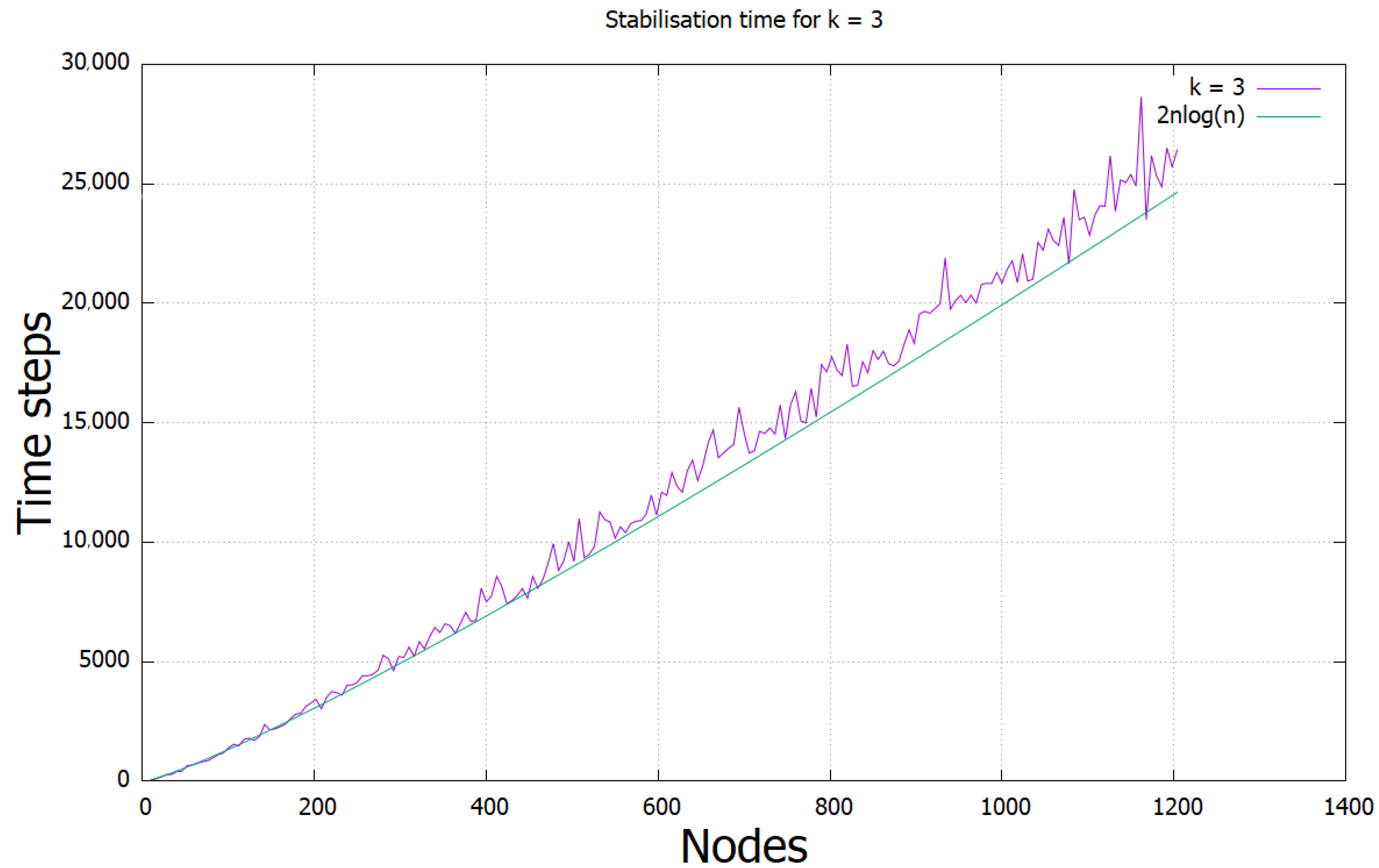
We now provide the results of simulating the protocol for $k=3$. We used the same conditions as in the other running time experiments, executing the protocol 10 times for each population size n, where $n=10+6t$, where t is the test number from 0 to 199. The results are given in Figure 1.

The running time is difficult to prove formally. This is because random variables are used, which represent the number of nodes with a given degree in a given time step. Their values depend on the values of all random variables in the previous time step. We, therefore, turn our focus to experiments based on measuring the impact of the value of k on the running time of the protocol.

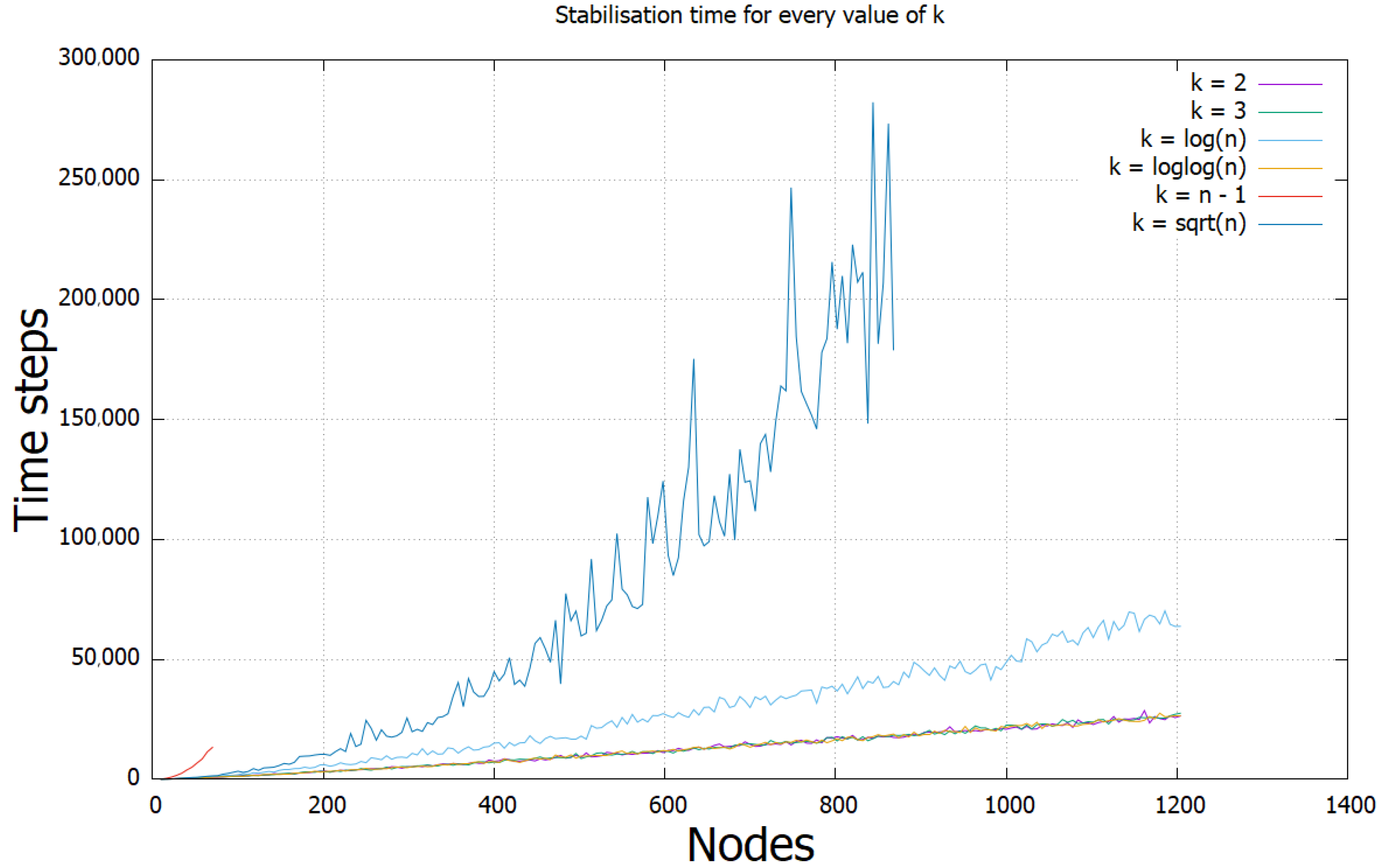
We measured the running time of our Cross-edges Tree protocol for different network sizes. The results below (Figure 2) show that a higher value of k has little effect on the running time until k exceeds $loglogn$.

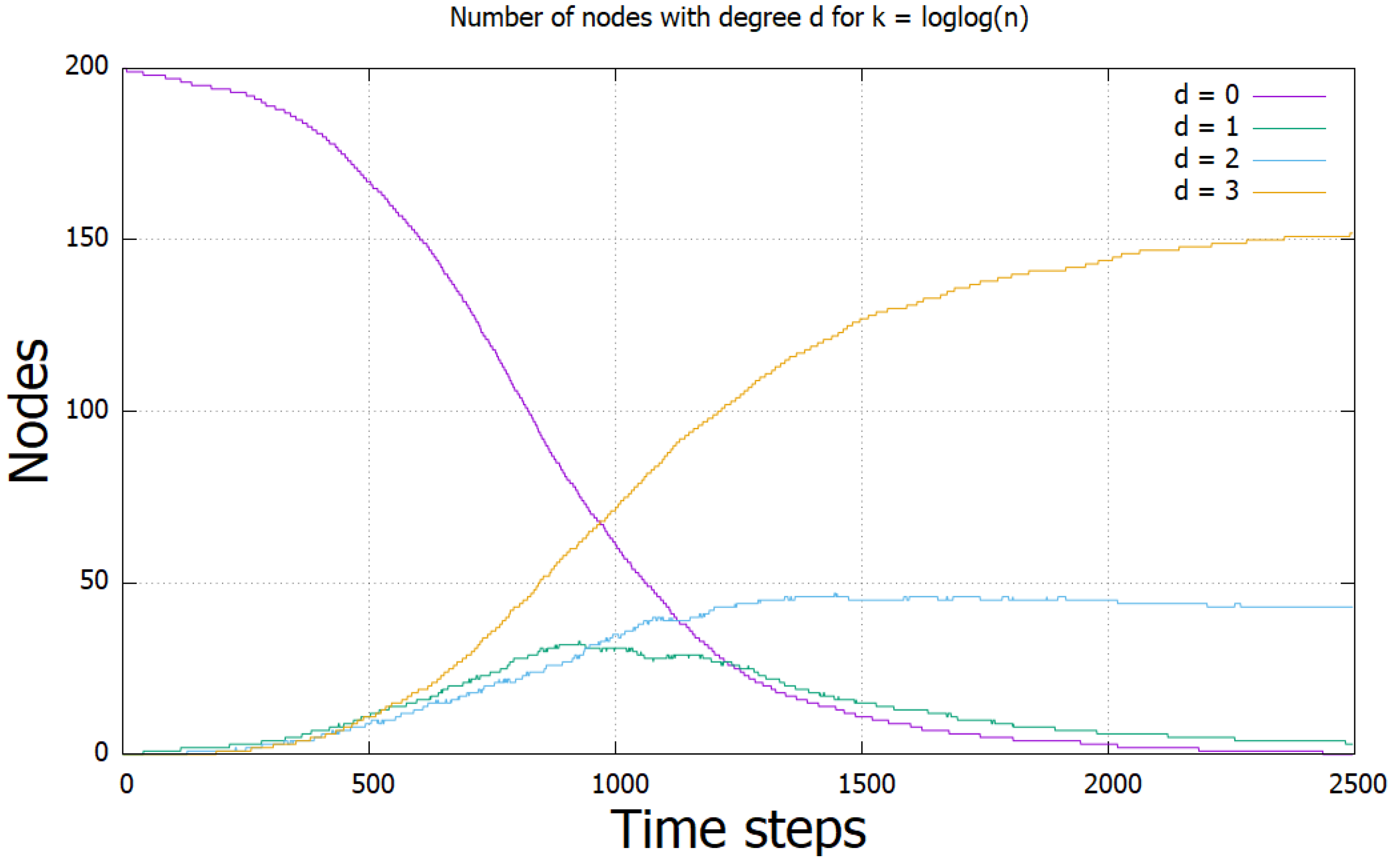
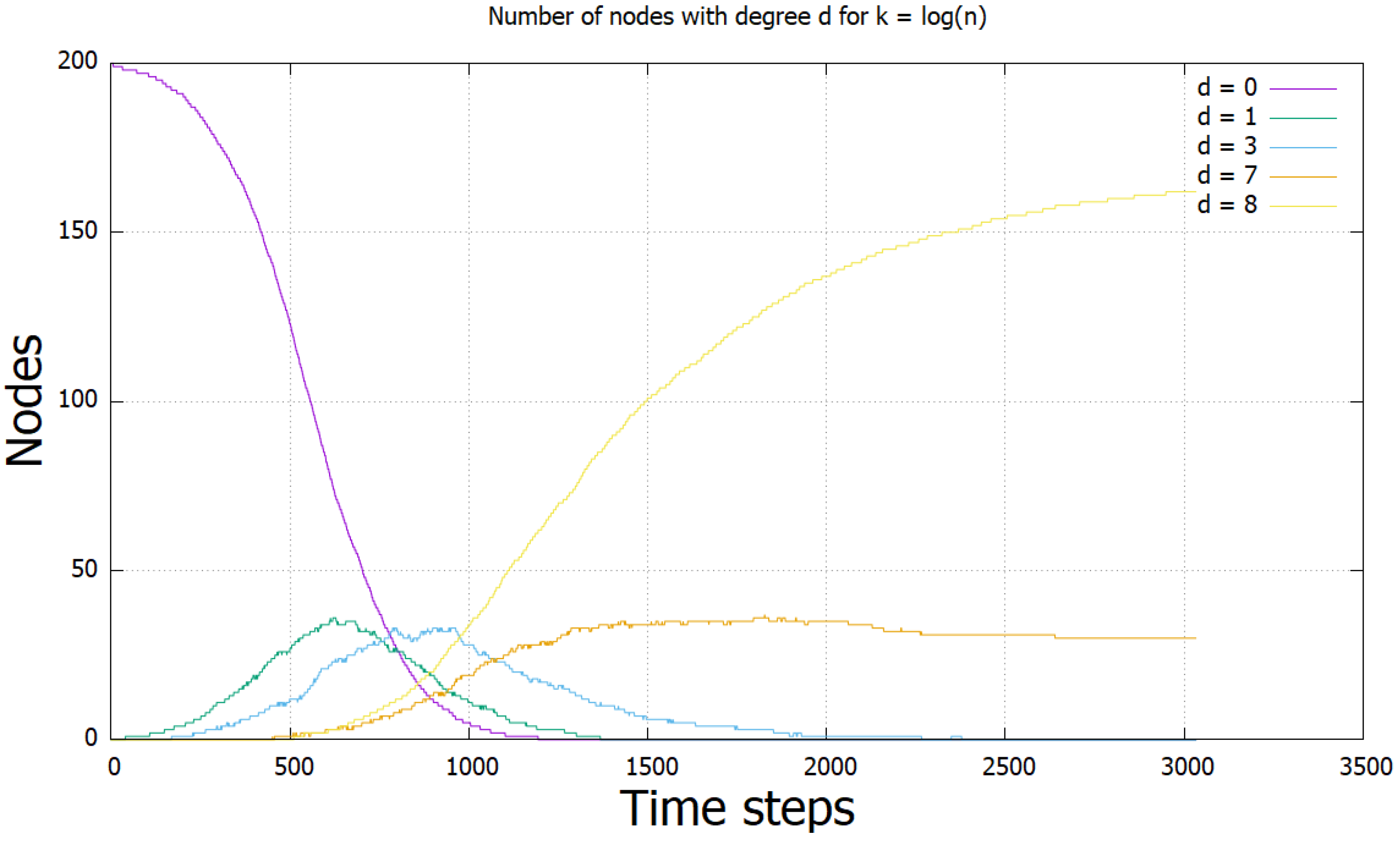
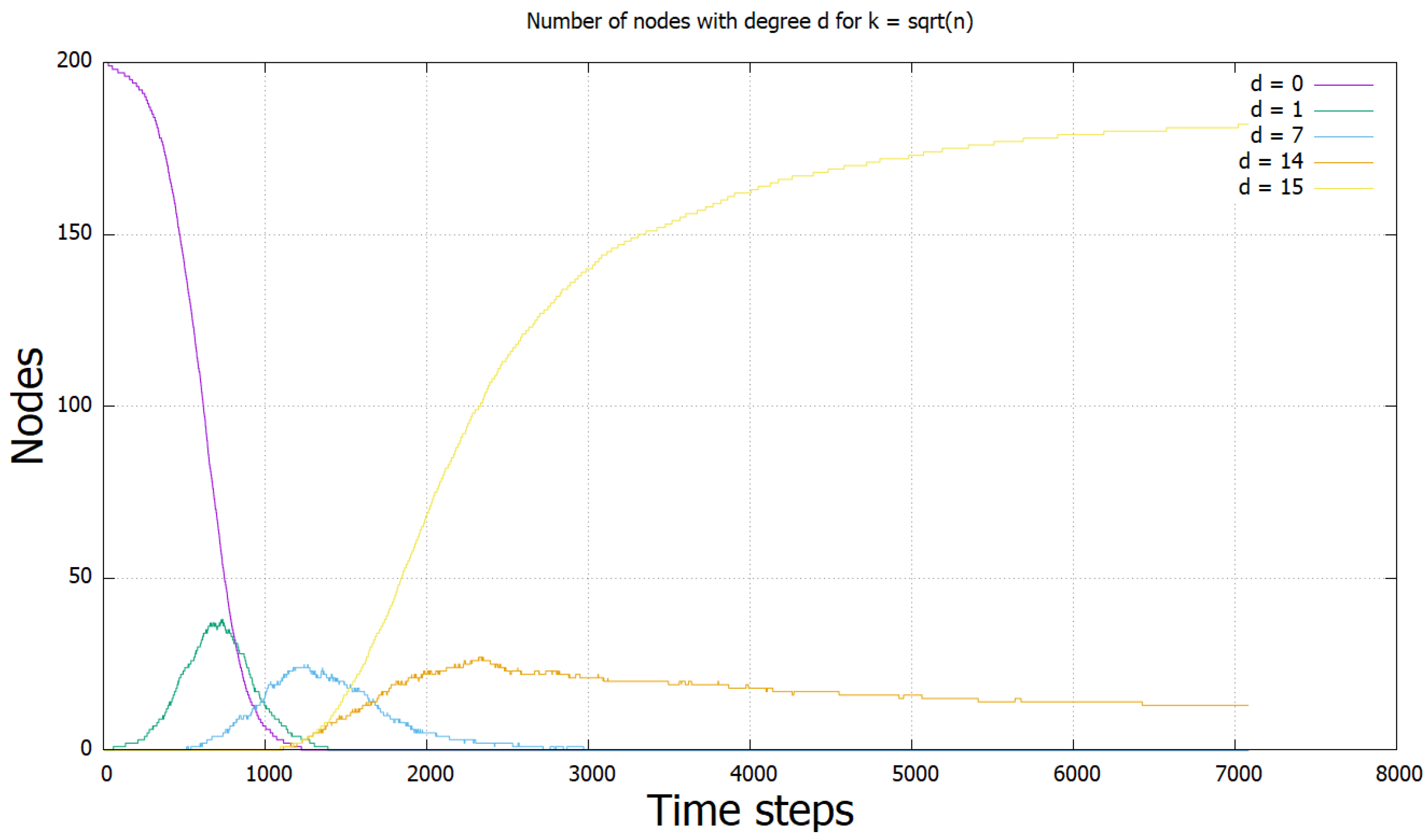
To investigate why the protocol slows down dramatically after this point, we ran experiments where we stored the number of nodes with specific degrees in each time step. We executed the protocol with 200 nodes, and ran 10 iterations. These degrees were set to 0, 1, $k/2$, $k-1$, and k. We collected results for $k=loglogn$ (Figure 3), $k=logn$ (Figure 4), and $k=\sqrt{n}$ (Figure 5). The results show that the cause seems to be a large reduction in the number of nodes, which are in the $k-1$ state as k grows as a fraction of n. They suggest that when the fraction of $k-1$ nodes is below some fraction between $1/4$ and $1/8$ of the total, the protocol slows down and enters the class of protocols with polynomial time.

4. Conclusions

Population protocols have a history of being applied in the context of physical devices [17]. However, to our knowledge, there has yet to be an attempt to apply the network constructors model to such a setting. For a cluster of devices, as in an Internet of Things style network [18], it may be desirable to form networks in order to solve problems in a very time-sensitive and highly dynamic context. This should typically be achieved without each device being aware of the size of the network or what specific devices the others are connected to. Network constructors and, thus, the protocols presented in this work, may be may be applicable to this, as they help define the class of networks which could be constructed in such a context. Works on social networks and social communities are a possible application domain for our models (see, e.g., [19]). It would be interesting to further investigate the potential applicability of population protocols and network constructors in data streaming applications; a preliminary attempt to do this was attempted by [20].

There are a number of open problems to be addressed. The most important is to develop an exact characterisation of the class of networks which can be constructed in polylogarthimic parallel time. However, there are other, more immediate problems. For example, we have yet to investigate the effect that widening the difference between k and l will have on the protocol. We speculate that this will result in a faster running time in exchange for less uniformity within the resulting spanning network. We also speculated about the possibilities of using a leaderless version of our Cross-tree Protocol. We believe that such a protocol may offer a trade off between the running time and the possibility of forming networks, which are spanning, depending on the values of k and l.

References

- Angluin, D.; Aspnes, J.; Diamadi, Z.; Fischer, M.J.; Peralta, R. Computation in networks of passively mobile finite-state sensors. Distrib. Comput. 2006, 18, 235–253. [Google Scholar] [CrossRef]
- Dan Alistarh, R.G. Polylogarithmic-time leader election in population protocols. In Proceedings of the 42nd International Colloquium on Automata, Languages, and Programming (ICALP), Kyoto, Japan, 6–10 July 2015; pp. 479–491. [Google Scholar]
- Gasieniec, L.; Stachowiak, G. Fast Space Optimal Leader Election in Population Protocols. In Proceedings of the 2018 Annual ACM-SIAM Symposium on Discrete Algorithms (SODA18), New Orleans, LA, USA, 7–10 January 2018; pp. 2653–2667. [Google Scholar]
- Alistarh, D.; Aspnes, J.; Eisenstat, D.; Gelashvili, R.; Rivest, R.L. Time-space trade-offs in population protocols. In Proceedings of the 2017 Annual ACM-SIAM Symposium on Discrete Algorithms (SODA17), Barcelona, Spain, 16–19 January 2017; pp. 2560–2579. [Google Scholar]
- Doty, D.; Eftekhari, M.; Michail, O.; Spirakis, P.G.; Theofilatos, M. Brief Announcement: Exact Size Counting in Uniform Population Protocols in Nearly Logarithmic Time. In Proceedings of the 32nd International Symposium on Distributed Computing (DISC), Schloss Dagstuhl–Leibniz-Zentrum fuer Informatik, New Orleans, LA, USA, 15–19 October 2018; pp. 46:1–46:3. [Google Scholar] [CrossRef]
- O’Dell, R.; Wattenhofer, R. Information dissemination in highly dynamic graphs. In Proceedings of the 2005 Joint Workshop on Foundations of Mobile Computing (DIALM-POMC), Cologne, Germany, 2 September 2005; pp. 104–110. [Google Scholar] [CrossRef]
- Kuhn, F.; Lynch, N.; Oshman, R. Distributed computation in dynamic networks. In Proceedings of the Forty-Second ACM Symposium on Theory of Computing (STOC), Cambridge, MA, USA, 5–8 June 2010; pp. 513–522. [Google Scholar]
- Michail, O.; Chatzigiannakis, I.; Spirakis, P.G. Causality, Influence, and Computation in Possibly Disconnected Synchronous Dynamic Networks. In Proceedings of the 16th International Conference on Principles of Distributed Systems (OPODIS), Rome, Italy, 18–20 December 2012; pp. 269–283. [Google Scholar]
- Angluin, D.; Aspnes, J.; Chen, J.; Wu, Y.; Yin, Y. Fast Construction of Overlay Networks. In Proceedings of the 17th ACM symposium on Parallelism in Algorithms and Architectures (SPAA), Las Vegas, NV, USA, 18–20 July 2005; pp. 145–154. [Google Scholar]
- Aspnes, J.; Shah, G. Skip Graphs. ACM Trans. Algorithms (TALG) 2007, 3, 37. [Google Scholar] [CrossRef]
- Aspnes, J.; Wu, Y. O(log n)-Time Overlay Network Construction from Graphs with Out-Degree 1. In Proceedings of the 11th International Conference on Principles of Distributed Systems (OPODIS), Guadeloupe, France, 17–20 December 2007; pp. 286–300. [Google Scholar]
- Götte, T.; Hinnenthal, K.; Scheideler, C. Faster Construction of Overlay Networks. In Proceedings of the 26th International Colloquium on Structural Information and Communication Complexity (SIROCCO), L’Aquila, Italy, 1–4 July 2019; pp. 262–276. [Google Scholar]
- Michail, O.; Skretas, G.; Spirakis, P.G. Distributed Computation and Reconfiguration in Actively Dynamic Networks. In Proceedings of the 39th ACM Symposium on Principles of Distributed Computing (PODC), Virtual Event, Italy, 3–7 August 2020; pp. 448–457. [Google Scholar]
- Michail, O.; Spirakis, P.G. Simple and efficient local codes for distributed stable network construction. Distrib. Comput. 2016, 29, 207–237. [Google Scholar] [CrossRef] [Green Version]
- Michail, O. Terminating distributed construction of shapes and patterns in a fair solution of automata. Distrib. Comput. 2018, 31, 343–365. [Google Scholar] [CrossRef] [Green Version]
- Gmyr, R.; Hinnenthal, K.; Scheideler, C.; Sohler, C. Distributed Monitoring of Network Properties: The Power of Hybrid Networks. In Proceedings of the 44th International Colloquium on Automata, Languages, and Programming (ICALP), Warsaw, Poland, 10–14 July 2017; pp. 137:1–137:15. [Google Scholar]
- Becchetti, L.; Bergamini, L.; Ficarola, F.; Salvatore, F.; Vitaletti, A. First Experiences with the Implementation and Evaluation of Population Protocols on Physical Devices. In Proceedings of the 2012 IEEE International Conference on Green Computing and Communications, Besancon, France, 20–23 November 2012; pp. 335–342. [Google Scholar] [CrossRef]
- Atzori, L.; Lera, A.; Morabito, G. The Internet of Things: A survey. Comput. Netw. 2010, 54, 2787–2805. [Google Scholar] [CrossRef]
- Holub, S.; Khymytsia, N.; Holub, M.; Fedushko, S. The Intelligent Monitoring of Messages on Social Networks. CEUR Workshop Proc. 2020, 2616, 308–317. [Google Scholar]
- Àlvarez, C.; Chatzigiannakis, I.; Duch, A.; Gabarró, J.; Michail, O.; Serna, M.; Spirakis, P.G. Computational models for networks of tiny artifacts: A survey. Comput. Sci. Rev. 2011, 5, 7–25. [Google Scholar] [CrossRef]
Figure 1.
Running time of the protocol for k = 3, compared with a polylogarithmic function.
Figure 2.
The effect of k on the running time of the protocol.
Figure 3.
The results for . Note the difference in the axes labels.
Figure 4.
The results for . Here, we see the beginning of a leftwards shift of the lines, and an upwards shift in .
Figure 5.
The results for . Both shifts are more intense.
Publisher’s Note: MDPI stays neutral with regard to jurisdictional claims in published maps and institutional affiliations. |
© 2021 by the authors. Licensee MDPI, Basel, Switzerland. This article is an open access article distributed under the terms and conditions of the Creative Commons Attribution (CC BY) license (https://creativecommons.org/licenses/by/4.0/).
Share and Cite
MDPI and ACS Style
Connor, M.; Michail, O.; Spirakis, P. On the Distributed Construction of Stable Networks in Polylogarithmic Parallel Time. Information 2021, 12, 254. https://0-doi-org.brum.beds.ac.uk/10.3390/info12060254
AMA Style
Connor M, Michail O, Spirakis P. On the Distributed Construction of Stable Networks in Polylogarithmic Parallel Time. Information. 2021; 12(6):254. https://0-doi-org.brum.beds.ac.uk/10.3390/info12060254
Chicago/Turabian StyleConnor, Matthew, Othon Michail, and Paul Spirakis. 2021. "On the Distributed Construction of Stable Networks in Polylogarithmic Parallel Time" Information 12, no. 6: 254. https://0-doi-org.brum.beds.ac.uk/10.3390/info12060254
Note that from the first issue of 2016, this journal uses article numbers instead of page numbers. See further details here.