Deep Hash with Improved Dual Attention for Image Retrieval

Abstract

Recently, deep learning to hash has extensively been applied to image retrieval, due to its low storage cost and fast query speed. However, there is a defect of insufficiency and imbalance when existing hashing methods utilize the convolutional neural network (CNN) to extract image semantic features and the extracted features do not include contextual information and lack relevance among features. Furthermore, the process of the relaxation hash code can lead to an inevitable quantization error. In order to solve these problems, this paper proposes deep hash with improved dual attention for image retrieval (DHIDA), which chiefly has the following contents: (1) this paper introduces the improved dual attention mechanism (IDA) based on the ResNet18 pre-trained module to extract the feature information of the image, which consists of the position attention module and the channel attention module; (2) when calculating the spatial attention matrix and channel attention matrix, the average value and maximum value of the column of the feature map matrix are integrated in order to promote the feature representation ability and fully leverage the features of each position; and (3) to reduce quantization error, this study designs a new piecewise function to directly guide the discrete binary code. Experiments on CIFAR-10, NUS-WIDE and ImageNet-100 show that the DHIDA algorithm achieves better performance.

1. Introduction

A great number of high-dimensional images and video data have been broadly used in various search engines and applications in recent years. This shows that quickly detecting the same image as a given query image from a large data set is an urgent problem to be solved [1,2]. It is common for deep hashing to be applied in data retrieval for its advantages of a solid learning ability and good portability [3]. Meanwhile, deep learning to hash methods [4,5,6,7,8,9,10,11] try to convert high-dimensional media data into compact binary code via a hash function, and the data structure information is stored in the Hamming space. Therefore, deep hashing methods garner attention in image retrieval.

Regarding early image retrieval methods, text-based image retrieval (TBIR) [12] uses the method of text annotation to describe the image content, and thus, the retrieval keywords of each image are formed. However, TBIR needs a lot of manual annotation, so it has gradually been replaced by content-based image retrieval (CBIR) [13,14]. In CBIR methods, the description between the image features is established by using a computer to analyze the image. However, there is an irreparable semantic gap between the feature description and high-level semantics. Deep hashing methods [4,5] can solve the limitation of CBIR, so the research on deep hashing is becoming more and more popular. Existing hashing methods are divided into two categories: data-independent hashing and data-dependent hashing. In the data-independent hashing methods [15], the binary code is generated by using the random projection matrix. Through theoretical analysis, it can be concluded that when the length of the binary codes increases, the hamming distance between the binary codes of two images gradually approaches the distance of feature space. However, long code is often required to achieve good performance, which wastes a lot of memory. By using the training data, data-dependent hashing methods [16,17,18,19,20,21,22,23,24] can generate more accurate binary code than data-independent hashing methods. Thus, data-dependent hashing has become more and more popular in real applications. This study explores data-dependent hashing methods to learn hash code with high quality.

Most deep hashing methods learn binary codes by exploring shallow CNN. The learned hash function is used to map the high-dimensional image features to the binary Hamming space. Such methods cause the following issues: (1) The goal of them is to optimize loss functions or reduce quantization error. However, they do not consider the correlation between the extracted deep features in the spatial dimension and channel dimension. (2) When using a shallow AlexNet network to extract features, the important feature information may be ignored. (3) Finally, the sign function is usually applied in the discrete optimization process of hash code, but the back-propagation algorithm cannot be implemented when the gradient of sign function is zero.

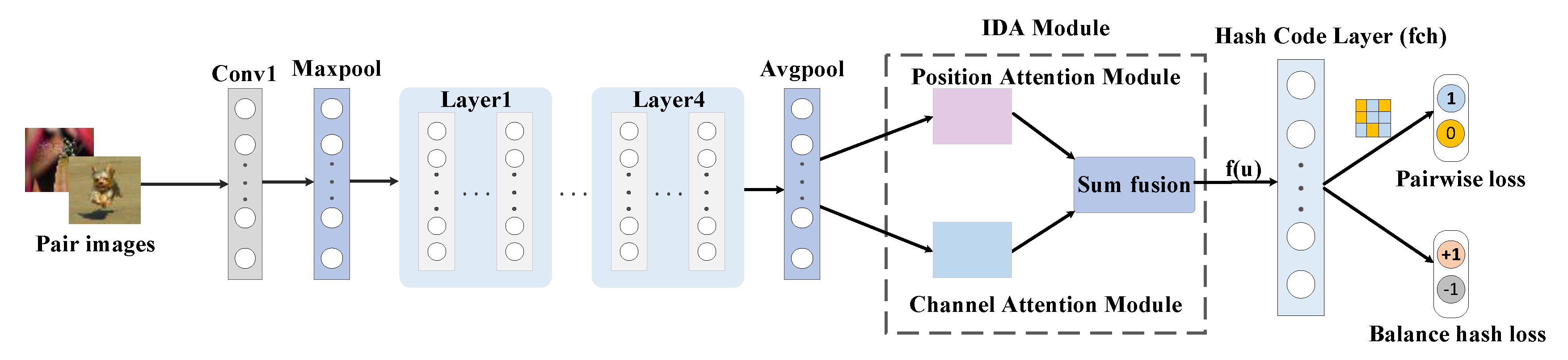
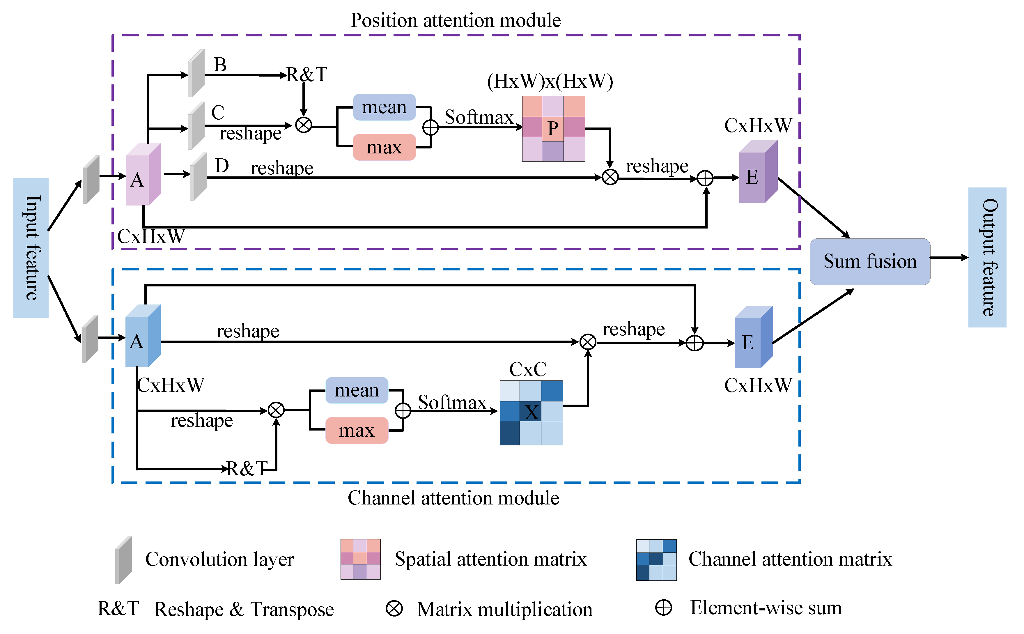
To optimize the above issues, this work is enlightened by the dual attention network for scene segmentation (DANet) [25], scene segmentation with dual relation-aware attention network [26], and GL-attention [27]; this study designs the IDA module on the basis of the position attention mechanism and channel attention mechanism, which can extract richer image features and obtain hash codes with strong discriminative ability. Specifically, as shown in Figure 1, this study uses ResNet18 as the network framework to extract features and then input them into the IDA module. Different from the DANet, as shown in Figure 2, to obtain the saliency and global information of the feature matrix and fully utilize the feature of each position, before calculating the spatial attention map $P$ and the channel attention map $X$, this study calculates the average value and maximum value of each column of the feature map matrix and combines the results of the two parts. In addition, the original feature map is subtracted to avoid feature redundancy. Finally, a new piecewise function is designed to process the network output into discrete binary code, which reduces quantization error. In the loss function part, a balance controlling loss is designed to balance the number of hash codes in the distribution of −1 and +1.

In short, our contributions are as follows:

• Firstly, this study designs an IDA module and embeds it in the ResNet18 network model, which learns feature representation and hash code learning at the same time. The position attention module is designed to capture the spatial interdependencies between features. The channel attention module is designed to model channel interdependencies.
• Secondly, to reduce quantization error, this study designs a new piecewise function to process the network output into discrete binary code.
• Thirdly, this study applies DHIDA on different loss functions, and measures its performance with extensive experiments on three standard image retrieval data sets.

The structure of the rest of the content is as follows. Section 2 discusses the related works. Section 3 mainly describes the network structure and the loss function. Section 4 precisely introduces the experiment and the results of the analysis. Section 5 draws the conclusion.

2. Related Work

Deep hashing for image retrieval is widely used in people’s daily lives [11,17,19]. For example, users can utilize an image to search for an image that meets their needs in many applications. Presently, generating more accurate hash code for each image has become a hot and difficult topic. Therefore, many existing methods explore the accuracy of hash codes from the perspective of the similarity matrix, feature representation and loss function. This section briefly discusses existing hash methods.

Data-dependent hashing methods include unsupervised hashing and supervised hashing. Unsupervised hashing methods train unlabeled data to learn hash functions that map raw data to binary code. Meanwhile, the similarity matrix is constructed by using the deep feature information. In unsupervised hashing methods, Weiss et al. [28] propose to save the manifold structure of the data set in Hamming space. However, this method is time consuming for calculating the affinity matrix. Hence, Liu et al. [29] utilize anchor graphs to obtain the processable low-rank adjacency matrices. Gong et al. [9] propose a method for reducing information loss by adding rotation zero-centered data. Owing to the absence of semantic label information, these unsupervised hash methods do not perform well. Supervised hashing methods directly explore the supervision information from data labels to construct the similarity matrix. In supervised hashing methods, Xia et al. [30] learn feature representation and hash code learning separately; there is no feedback between the two parts. On this basis, Lai et al. [31] propose to learn deep semantic features and hash code in the process of joint learning. Li et al. [5] utilize the end-to-end network to consider the common application scenario of pairwise labels. Inspired by Li et al., Wang et al. [32] propose to maximize the likelihood of the triple label to evaluate the quality of hash codes. To further mine data labels and narrow the gap between the Hamming distance and its substitution, Zhu et al. [33] propose the bi-modal Laplacian prior to learning the continuous representation and high-quality hash code. Meanwhile, Cao et al. [34] develop a CNN network with a non-smooth binary activation function to solve the problem of gradient disappearance. In addition, weighted data labels are used to solve the problem of data imbalance. Based on their prior efforts [34] to address the data labels imbalance, Cao et al. [35] propose a probability function based on the Cauchy distribution to tackle the misspecification problem of the sigmoid function. Zhang et al. [36] propose to rank the similarity of pairwise images with multiple labels. To further reduce quantization error, Zheng et al. [18] propose that CNN directly outputs the binary code, and the straight-through estimator is designed to optimize the network in the process of discrete gradient propagation. This pairwise or triplet based on hash learning leads to low efficiency of the similarity analysis. Hence, in the method proposed by Yuan et al. [7], the similarity center of each class is constructed by using the Hadamard matrix and the Bernoulli distributions. The binary cross entropy loss is employed to minimize the distance within the class and maximize the distance between the classes. To reduce the retrieval time and improve the retrieval speed, Zhang et al. [37] use tree structures to generate the deep hash code and prune the irrelevant branches to reduce the retrieval time.

In summary, most of the existing hash methods only consider the part of optimizing the loss function, while ignoring the shortcomings of using CNN to extract image feature information. Encouraged by the dual attention model [25,26,27], this study designs the IDA module, which includes the position attention module and channel attention module. The position attention module promotes the feature representation ability, and the channel attention module establishes the interdependence between the channels. Combining the output of the two modules can fully extract the crucial semantic information of the image. In addition, this study designs a piecewise function to quantify the network output.

3. Deep Hash with Improved Dual Attention

In this section, this paper describes the research method, the structure of the network model, the details of the IDA module and the process of optimizing the network.

3.1. Problem Formulation

In the similarity retrieval, given $n$ image samples, $X={\left\{x_i\right\}}_{i=1}^n$ and its corresponding data labels are expressed as $Y={\left\{y_i\right\}}_{i=1}^c$, where $x_i$ represents the $it\mathit{h}$ image, $y_i$ represents the data labels of the $it\mathit{h}$ image, and $c$ is the number of categories in the data set. The similarity matrix $S=\left\{s_{ij}\right\}$ is constructed from data labels $y$. where $s_{ij}=1$ if $x_i$ and $x_j$ are similar, and $s_{ij}=0$ otherwise.

The deep hash aims to learn a nonlinear hash function $F:x\to \mathit{h}\in {\left\{-1,+1\right\}}^K$, which transforms the deep feature representation of each image $x_i$ into K-dimensional representation ${\mathit{u}}_{\mathit{i}}$. To reduce quantification error, this study defines a new piecewise function for processing ${\mathit{u}}_{\mathit{i}}$. Specifically, a threshold value of the binary code is set to $\left[-1,1\right]$, and then it deals with the output that exceeds the threshold value. This study considers the output beyond the threshold as 1, and the output below the threshold as −1. This piecewise function is described as follows:

$$f\left({\mathit{u}}_{\mathit{i}}\right)=\{\begin{array}{c}1, {\mathit{u}}_{\mathit{i}}>1 \\ {\mathit{u}}_{\mathit{i}}, -1<{\mathit{u}}_{\mathit{i}}<1 \\ -1, {\mathit{u}}_{\mathit{i}}<-1 \end{array}$$

(1)

where ${\mathit{h}}_{\mathit{i}}=sign\left(f\left({\mathit{u}}_{\mathit{i}}\right)\right)$ is used to quantize ${\mathit{u}}_{\mathit{i}}$ into K-bit binary code ${\mathit{h}}_{\mathit{i}}\in {\left\{-1,1\right\}}^K$, where $K$ is the length of hash code and $sign()$ is the sign function, which is defined as follows:

$$sign\left(x\right)=\{\begin{array}{c}1, if x\ge 0 \\ -1, ot\mathit{h}erwise \end{array}$$

(2)

3.2. Network Framework

The network framework is illustrated in Figure 1. In order to obtain sufficient features with contextual information, this study applies ResNet18 as the basic backbone network and embeds the IDA modules in it, meanwhile, replacing the classification layer of ResNet18 with a hash layer. After the network becomes deeper, this study employs the Rectified Linear Unit (ReLU) activation function to solve the disappearance of the gradient.

The details for the IDA module are shown in Figure 2, which is comprised of a position attention module and channel attention module.

In the position attention module, the self-attention mechanism is introduced to establish the spatial dependence between any two locations in the feature matrix. The feature of a specific location is updated by weighted summation of the aggregate features of all locations, and its weight is determined by the similarity between features. If the features of any two locations (regardless of their distance in spatial dimensions) have a similar relationship, then the two locations can promote each other. Therefore, the role of the position attention mechanism is to capture salient information from contextual features and encode them into local features, on which a wider range of context relations are established, thus improving the feature representation ability.

In the channel attention module, the self-attention mechanism is also introduced to capture the channel dependency between any two channel maps, and the weighted sum of maps of all channels is used to update the maps of each channel. By using the dependency relationship between different channels, the channel attention module can enhance the interdependence of the feature channels and improve the feature representation of the feature semantics. The role of the channel attention module is to selectively integrate the highly dependent channels and improve the semantic feature expression. Meanwhile, the long-distance semantic dependency between the different channels is modelled.

Finally, the outputs of the two attention modules are fused to gain better pixel-level prediction feature representations.

3.3. IDA Module

This section mainly introduces the content of the IDA module and the improvement of the two attention modules.

3.3.1. Position Attention Module

The function of the position attention module is to establish the spatial correlation for any two positions of the feature map by introducing the self-attention mechanism.

As shown in Figure 2, firstly, the high-dimensional features are fed into a convolution layer to obtain a feature map $A\in {ℝ}^{C\times \mathit{H}\times \mathit{W}}$. $A$ is fed into three convolution layers to obtain the three feature maps $B$, $C$ and $D$, where $\left\{B,C,D\right\}\in {ℝ}^{C\times \mathit{H}\times \mathit{W}}$. Then, they are reshaped into ${ℝ}^{C\times N}$, where $N=\mathit{H}\times \mathit{W}$ is the total number of pixels. Secondly, this paper multiplies the transpose of $B$ by $C$ to generate $M_{ij}\in {ℝ}^{N\times N}$. Finally, encouraged by [27], to compute the salient and global features of the feature map, and to take full advantage of the features of each position, $M_{ij}$ is processed as follows:

$${\tilde{M}}_{ij}=\frac{\max \left(M_{ij} \right)+mean\left(M_{ij} \right)}{2}-M_{ij}$$

(3)

Using the maximum or mean function alone may cause fine-grained features to be ignored, so this study employs two functions in parallel. The spatial attention map $P\in {ℝ}^{N\times N}$ is generated by entering ${\tilde{\mathrm{M}}}_{ij}$ into the SoftMax layer. Each element of the calculated $P$ matrix is as follows:

$$P_{ji}=\frac{exp\left({\tilde{M}}_{ij}\right)}{{{\displaystyle \sum }}_{i=1}^{N}exp\left({\tilde{M}}_{ij}\right)}$$

(4)

where $P_{ij}$ represents the effect of the $ith$ position on the $jth$ position. The larger the $P_{ij}$, the higher the correlation between the two positions. Meanwhile, this study multiplies the transpose of $P$ with $D$ and reshapes the product to the original shape. Finally, the output$E\in {ℝ}^{C\times \mathit{H}\times \mathit{W}}$ is obtained as follows:

$$E_i=\alpha {\displaystyle \sum }_{i=1}^N\left(P_{ji}{D}_i\right)+A_j$$

(5)

where $\alpha$ is a scale parameter [38] initialized to 0 and gradually assigns weight by learning. $D_i$ is the $ith$ feature of $D$, $A_j$is the $jth$ feature of $A$, and $E_i$ is the $ith$ feature of $E$. Every position feature of $E_i$ is related to the global feature of $E$ and the original features. Therefore, $E$ has global contextual features information, so it establishes the spatial relationship between any two positions.

3.3.2. Channel Attention Module

The channel attention module captures the interdependence between any two channels maps by exploring the self-attention mechanism.

As shown in Figure 2, according to feature map $A\in {ℝ}^{C\times \mathit{H}\times \mathit{W}}$, $A$ is reshaped to $A_1\in {ℝ}^{C\times N}$ and express the transpose of $A_1$ as $A_1^T\in {ℝ}^{N\times C}$. Then, this study directly performs a matrix multiplication between $A_1$ and $A_1^T$ to obtain matrix $N_{ij}$. Meanwhile, $N_{ij}$ is also processed similar to Equation (3), as shown below:

$${\tilde{N}}_{ij}=\frac{max\left(N_{ij}\right)+mean\left(N_{ij}\right) }{2}-N_{ij}$$

(6)

Then, put ${\tilde{N}}_{ij}$ into the SoftMax layer to obtain the channel attention map $X\in {ℝ}^{C\times C}$. Each element of the $X$ matrix is calculated as follows:

$$X_{ji}=\frac{exp\left({\tilde{N}}_{ij}\right)}{{{\displaystyle \sum }}_{i=1}^{C}exp\left({\tilde{N}}_{ij}\right)}$$

(7)

where $X_{ji}$ indicates the influence of the $ith$ channel on the $jth$ channel. Therefore, $X$ represents the connection between a certain channel and other channels. Next, this approach can improve the expression of semantic features by performing the $X$ multiplied by $A$ operation. Then, the output $E\in {ℝ}^{C\times \mathit{H}\times \mathit{W}}$ is obtained as follows:

$$E_j=\beta {\displaystyle \sum }_{i=1}^N\left(X_{ji}{A}_i\right)+A_j$$

(8)

where$\beta$is a scale parameter initialized to 0 and gradually assigns weight by learning. $E_j$ is the $jth$ feature of $E$. $A_j$ is the $jth$ channel of $A$. The resultant $E$ of each channel is related to the features of all channels and original features. Hence, $E$ establishes the connection between the channels and improves the discrimination ability of features.

Finally, the outputs of the two modules are sum fused, which strengthens the dependency relationship between pixels and enhances the dependency relationship between channels. Therefore, the output of the IDA module can obtain better pixel-level prediction feature representation.

3.4. Model Formulation

For pairwise binary hash code ${\mathit{h}}_{\mathit{i}}$ and ${\mathit{h}}_{\mathit{j}}$, the Hamming distance can be calculated as $D\left({\mathit{h}}_{\mathit{i}},{\mathit{h}}_{\mathit{j}}\right)=\frac{1}{2}\left(K-{\mathit{h}}_{\mathit{i}},{\mathit{h}}_{\mathit{j}}\right)$, where ${\mathit{h}}_{\mathit{i}},{\mathit{h}}_{\mathit{j}}=\frac{1}{2}{\mathit{h}}_i^T{\mathit{h}}_{\mathit{j}}$ means the inner product, and$K$ is the length of the hash code. This shows that the change of inner product and Hamming distance are opposite. When the inner product increases, the Hamming distance decreases. Therefore, it is more intuitive to judge the similarity of two images by the inner product. The similarity matrix $S=\left\{s_{ij}\right\}$composed of image labels is given, and the logarithm maximum posteriori estimation of hash code $\mathit{H}=\left[{\mathit{h}}_1,\dots ,{\mathit{h}}_{\mathit{n}}\right]$ is described as follows:

$$logP\left(\mathit{H}|S\right)\propto logp\left(S|\mathit{H}\right)p\left(\mathit{H}\right)={\displaystyle \sum }_{s_{ij}\in S}logp\left(s_{ij}|{\mathit{h}}_{\mathit{i}},{\mathit{h}}_{\mathit{j}}\right)p\left({\mathit{h}}_{\mathit{i}}\right)p\left({\mathit{h}}_{\mathit{j}}\right)$$

(9)

where $p(S|\mathit{H})$ is the likelihood function, $p\left(\mathit{H}\right)$ is the prior distribution and $p(s_{ij}|{\mathit{h}}_{\mathit{i}},{\mathit{h}}_{\mathit{j}})$ is the conditional probability of the similarity label $s_{ij}$ under the given premise of ${\mathit{h}}_{\mathit{i}},{\mathit{h}}_{\mathit{j}}$, which is defined as the following pairwise logistic function:

$$\begin{gathered} p\left(s_{ij}|{\mathit{h}}_{\mathit{i}},{\mathit{h}}_{\mathit{j}}\right)=\{\begin{array}{c}\sigma (\langle {\mathit{u}}_i,{\mathit{u}}_j\rangle ), s_{ij}=1\\ 1-\sigma (\langle {\mathit{u}}_i,{\mathit{u}}_j\rangle ), s_{ij}=0\end{array} \\ =\sigma {(\langle {\mathit{u}}_i,{\mathit{u}}_j\rangle )}^{s_{ij}}{\left(1-\sigma (\langle {\mathit{u}}_i,{\mathit{u}}_j\rangle )\right)}^{1-s_{ij}} \end{gathered}$$

(10)

where $\sigma \left(\phi \right)=\frac{1}{1+e^{-\phi }}$ is the sigmoid function and ${\mathit{h}}_{\mathit{i}}=sign({\mathit{u}}_{\mathit{i}})$. Equation (10) shows that the inner product becomes larger, and the conditional probability $p\left(1|{\mathit{h}}_{\mathit{i}},{\mathit{h}}_{\mathit{j}}\right)$ also increases, which indicates that hash code ${\mathit{h}}_{\mathit{i}} \mathrm{and} {\mathit{h}}_{\mathit{j}}$ are similar. The larger $p\left(0|{\mathit{h}}_{\mathit{i}},{\mathit{h}}_{\mathit{j}}\right)$ is, the more dissimilar the hash code ${\mathit{h}}_{\mathit{i}},{\mathit{h}}_{\mathit{j}}$ is.

In order to calculate the pairwise similarity loss, the negative maximum likelihood function of Equation (10) is computed, and we take its logarithmic as follows:

$$L_1={\displaystyle \sum }_{S_{ij}ϵS}\left(log\left(1+exp(\langle {\mathit{u}}_{\mathit{i}},{\mathit{u}}_j\rangle )\right)-s_{ij}(\langle {\mathit{u}}_{\mathit{i}},{\mathit{u}}_{\mathit{j}}\rangle )\right)$$

(11)

Finally, inspired by [10,16], this study adopts a balance controlling loss to address the problem of the imbalanced hash code distribution. This means that the binary code is evenly distributed in the number of -1 and +1. Therefore, all of the bits of the binary code are equally used. The definition of the balance controlling is as follows:

$$L_2={\displaystyle \sum }_{n=1}^K{\left|mean\left({\mathit{u}}_{\mathit{i}}^{\left(n\right)}\right)\right|}^2$$

(12)

where ${\mathit{u}}_{\mathit{i}}^{\left(n\right)}$ is the $n^{th}$ element of the hash code ${\mathit{u}}_{\mathit{i}}$.

Finally, the total loss function can be summarized as follows:

$$minL=L_1+\gamma L_2={\displaystyle \sum }_{S_{ij}ϵS}\left(log\left(1+exp(\langle {\mathit{u}}_{\mathit{i}},{\mathit{u}}_j\rangle )\right)-s_{ij}(\langle {\mathit{u}}_{\mathit{i}},{\mathit{u}}_{\mathit{j}}\rangle )\right)+\gamma {\displaystyle \sum }_{n=1}^K{\left|mean\left({\mathit{u}}_{\mathit{i}}^{\left(n\right)}\right)\right|}^2.$$

(13)

where $\gamma$is the weight balance hyperparameter. According to the model method proposed in this paper, extensive experiments show that the result of the experiment is the best when the value of $\gamma$ is 0.1. It is only for the experimental data of this study.

3.5. Learning

The whole training process of the DHIDA model is shown in Algorithm 1. In the DHIDA method, the loss function can be effectively optimized via the backpropagation (BP) algorithm. Learning a hash function through an end-to-end network to map the training images into the binary codes, it is set as follows:

$${\mathit{u}}_{\mathit{i}}={\mathit{W}}^T\psi \left(x_i;\theta \right)+\mathit{b}$$

(14)

where $\theta$ is the parameters of the feature layers, $\psi \left(x_i;\theta \right)$ is the output of the full layers related to image $x_i$, and ${\mathit{W}}^T\in {ℝ}^{4096\times K}$ presents the transpose of the weight matrix. $\mathit{b}\in {ℝ}^K$ denotes the bias vector, where $K$ is the length of the binary code and ${\mathit{u}}_{\mathit{i}}$ is the network output. In the DHIDA model, the parameters to be optimized include $\mathit{W}$, $\mathit{b}$, $\theta$ and H. This study adopts the control variable method to optimize the parameters.

Then, ${\mathit{h}}_{\mathit{i}}$ is optimized as follows:

$${\mathit{h}}_{\mathit{i}}=sign\left({\mathit{u}}_{\mathit{i}}\right)$$

(15)

For the other parameters $\mathit{W}$, $\mathit{b}$, and $\theta$, by calculating the derivative of the total loss $L$ to ${\mathit{u}}_{\mathit{i}}$ in Equation (13), we can obtain the following:

$$\frac{\partial L}{\partial {\mathit{u}}_{\mathit{i}}}=\frac{1}{2}{\displaystyle \sum }_{S_{ij}ϵS}{a}_{ij}-S_{ij}{\mathit{u}}_{\mathit{j}}+\frac{1}{2}{\displaystyle \sum }_{S_{ij}ϵS}{a}_{ji}-S_{ji}{\mathit{u}}_{\mathit{j}}+2\gamma \left(mean\left({\mathit{u}}_{\mathit{i}}^{\left(n\right)}\right)\right)$$

(16)

where ${\mathrm{a}}_{ij}=\sigma \left(\frac{1}{2}{\mathit{u}}_i^T{\mathit{u}}_j\right)$.

For the update of parameters $\mathit{W}$, $\mathit{b}$, and $\theta$, this study chooses to fix two of them to update the other. Therefore, their derivatives are calculated as follows:

$$\frac{\partial L}{\partial \mathit{W}}=\psi \left(x_i;\theta \right){\left(\frac{\partial L}{\partial {\mathit{u}}_{\mathit{i}}}\right)}^T,$$

(17)

$$\frac{\partial L}{\partial v}=\frac{\partial L}{\partial {\mathit{u}}_{\mathit{i}}},$$

(18)

$$\frac{\partial L}{\psi \left(x_i;\theta \right)}=\mathit{W}\frac{\partial L}{\partial {\mathit{u}}_{\mathit{i}}}$$

(19)

The learning process of the DHIDA model is shown in Algorithm 1.

Algorithm 1. DHIDA.

Input:   Given $X={\left\{x_i\right\}}_{i=1}^n$$\mathrm{and} S=\left\{s_{ij}\right\}$. Output:   Updated parameters $\mathit{W}, \mathit{b}, \theta and$H. Initialization:   Initialize the ResNet18 model;   Initialize parameters $\theta$ from the pre-trained ResNet18 model;   Randomly sampled $\mathit{W}$$\mathrm{and} \mathit{b}$ from Gaussian distribution. Repeat:   Randomly select a mini batch of images from $X$. Execute the following actions for each image $x_i$,:   Calculate $\psi \left(x_i;\theta \right)$ by forward backpropagation;   Calculate ${\mathit{u}}_{\mathit{i}}={\mathit{W}}^T\psi \left(x_i;\theta \right)+\mathit{b}$;   Calculate hash code of $x_i$$\mathrm{with} {\mathit{h}}_i=sgn\left({\mathit{u}}_{\mathit{i}}\right)$ and derivatives for $\mathit{W}, \mathit{b} \mathrm{and} \theta$ according to (17), (18) and (19);   Update the parameters $\mathit{W}, \mathit{b}, \theta ;$ Until iterations completed

Finally, the trained ResNet18 model is obtained for the final deep hashing model, and the binary code corresponding to images can be generated by Equation (14).

4. Experiments

This section mainly describes the introduction of the experimental data sets, evaluation metrics, parameters setting, the result of the analysis and the empirical analysis.

4.1. Data Sets

This study conducts experimental evaluations on three public data sets: CIFAR-10, NUS-WIDE and ImageNet-100.

1. CIFAR-10 contains 60,000 RGB color images belonging to 10 categories. It is a single-label data set with 6000 images in each category. In this experiment, the training set is formed by randomly sampling 500 images in each category (5000 images in all), and 100 images (1000 images in all) are randomly selected in each category to form the test set. The rest of the images serve as the database for retrieval.

2. NUS-WIDE is a multi-label data set containing 269,648 images. This study adopts 195,834 images that are associated with the 21 categories. Among them, 100 images are randomly selected from each class (2100 images in all) as the test set and the remaining images as the database. Furthermore, in the database, the experiments select 500 images from each category (10,500 images in all) as the training set.

3. ImageNet-100 contains 128,503 single-label images, and each image belongs to one of 100 categories. In this experiment, 5000 images are randomly selected to serve as the test set, and the rest of the images serve as the database. Meanwhile, the experiments choose 130 images from each category (13,000 in all) of the database as the training set to train the model.

4.2. Evaluation Metrics and Settings

In the experiment, this study compares DHIDA with eight classic hashing methods, which include DBDH [18], HashNet [34], IDHN [36], DFH [39], DSH [17], DSDH [20], DHN [33] and LCDSH [40].

This study evaluates the image retrieval quality of DHIDA with four metrics: mean average precision (mAP), precision–recall curves (PR), precision curves within Hamming distance 2 (P@H = 2) and precision curves of the first 1000 retrieval results (P@N). In order to compare all the methods fairly, this experiment adopts mAP@ALL for CIFAR-10, mAP@5000 for NUS-WIDE and mAP@1000 for ImageNet-100.

For fair comparison, the experiments replace the backbone network of all comparison methods with the pre-trained ResNet18 network and use the Pytorch framework to reproduce the codes. The parameter information of each layer is illustrated in

Table 1. Configuration of each layer in DHIDA method.

Layers	Configuration
Conv1	{64 × 112 × 112, k = 7 × 7, s = 2 × 2, p = 3 × 3, ReLU}
Maxpool	{64 × 54 × 54, k = 3 × 3, s = 2 × 2, p = 1 × 1, ReLU}
Layer1	{64 × 56 × 56, k = 3 × 3, s = 1 × 1, p = 1 × 1, ReLU} × 4
Layer2	{128 × 28 × 28, k = 3 × 3, s = 2 × 2, p = 1 × 1, ReLU} × 4
Layer3	{256 × 14 × 14, k = 3 × 3, s = 2 × 2, p = 1 × 1, ReLU} × 4
Layer4	{512 × 7 × 7, k = 3 × 3, s = 2 × 2, p = 1 × 1, ReLU} × 4
Avgpool	512 × 1 × 1
fch	K, the length of hash code

. The network contains 18 layers (conv1 + Layer1~Layer4 + fch) in total, and each layer contains four convolution layers. Among them, the small letters are as follows: p denotes the size of the convolution kernel, s and k represent the stride and padding, respectively, and fch represents the hash code layer. The features extracted from the ResNet18 network would be fed into the IDA module.

This study updates the parameters of convolutional layers and fully connected layer copy from ResNet18 pre-trained model by BP. All methods utilize the same training set and test set. Furthermore, the network model is optimized by the root mean square prop (RMSProp), the learning rate is set as $5\times {10}^{-5}$, the mini batch size of images is set as 128 and the weight decay parameter is set as $1\times {10}^{-5}$.

The experimental environment configuration information is illustrated in

Table 2. Configuration information.

Item	Configuration
OS	Ubuntu 16.04 (×64)
GPU	Tesla V100

.

4.3. Results Analysis

As shown in

Table 3. mAP for different number of bits on three data sets.

Method	CIFAR-10 (mAP@ALL)				NUS-WIDE (mAP@5000)				Imagenet-100 (mAP@1000)
	16 bit	32 bit	48 bit	64 bit	16 bit	32 bit	48 bit	64 bit	16 bit	32 bit	48 bit	64 bit
DHIDA	0.8213	0.8359	0.8420	0.8428	0.8278	0.8414	0.8519	0.8552	0.6346	0.6296	0.6573	0.6870
DBDH	0.8021	0.8113	0.8129	0.8209	0.8150	0.8360	0.8442	0.8484	0.3358	0.3215	0.5626	0.6321
DSDH	0.7761	0.7881	0.8086	0.8183	0.8085	0.8373	0.8441	0.8441	0.1612	0.3011	0.3638	0.4268
DHN	0.7695	0.7871	0.7869	0.7966	0.8108	0.8069	0.7854	0.7910	0.4900	0.4808	0.4747	0.5664
LCDSH	0.7383	0.7661	0.8083	0.8202	0.8071	0.8304	0.8425	0.8436	0.2269	0.3177	0.4517	0.4671
HashNet	0.6975	0.7892	0.7878	0.7949	0.7453	0.8180	0.8361	0.8297	0.3017	0.4690	0.5400	0.5719
IDHN	0.6641	0.7296	0.7762	0.7682	0.7820	0.7795	0.7601	0.7366	0.2721	0.3255	0.4477	0.5539
DFH	0.5947	0.6347	0.7298	0.7662	0.7893	0.8185	0.8350	0.8372	0.1727	0.3435	0.3445	0.3430
DSH	0.5095	0.4663	0.4702	0.4714	0.6680	0.7383	0.7563	0.7940	0.3109	0.3848	0.4294	0.4403

, the experiments calculate the mAP value of DHIDA and other comparison methods on CIFAR-10, NUS-WIDE and ImageNet-100. The length of the hash code is 16, 32, 48 and 64 bits, respectively. From the results in Table 3, the mAP of DHIDA is obviously higher than the other comparison algorithms.

Specifically, on the CIFAR-10 data set, the mAP of DHIDA in different length hash codes achieves 82.13%, 83.59%, 84.20% and 84.28% in Table 3. Compared with DBDH, DHIDA can achieve absolute boosts of 1.9%, 2.5%, 2.9% and 2.2%. On the NUS-WIDE data set, compared with DBDH, the mAP of DHIDA improves by 1.3%, 0.5%, 0.8% and 0.7% at 16, 32, 48 and 64 bits. On ImageNet-100, compared with DBDH, the mAP of DHIDA improves by 29.9%, 30.8%, 9.5% and 5.5% on different bits. Therefore, compared with the highest mAP results, this study achieves increases of 2.4%, 0.8% and 18.9% in average mAP for different bits on the three data sets, respectively. Compared with the classic algorithm HashNet, there is an average increase of 6.8%, 3.6%, and 18.1% on CIFAR-10, NUS-WIDE, and ImageNet-100. Hence, the experimental results show that the algorithm can fully mine the contextual semantic information of the features and generate high-quality codes.

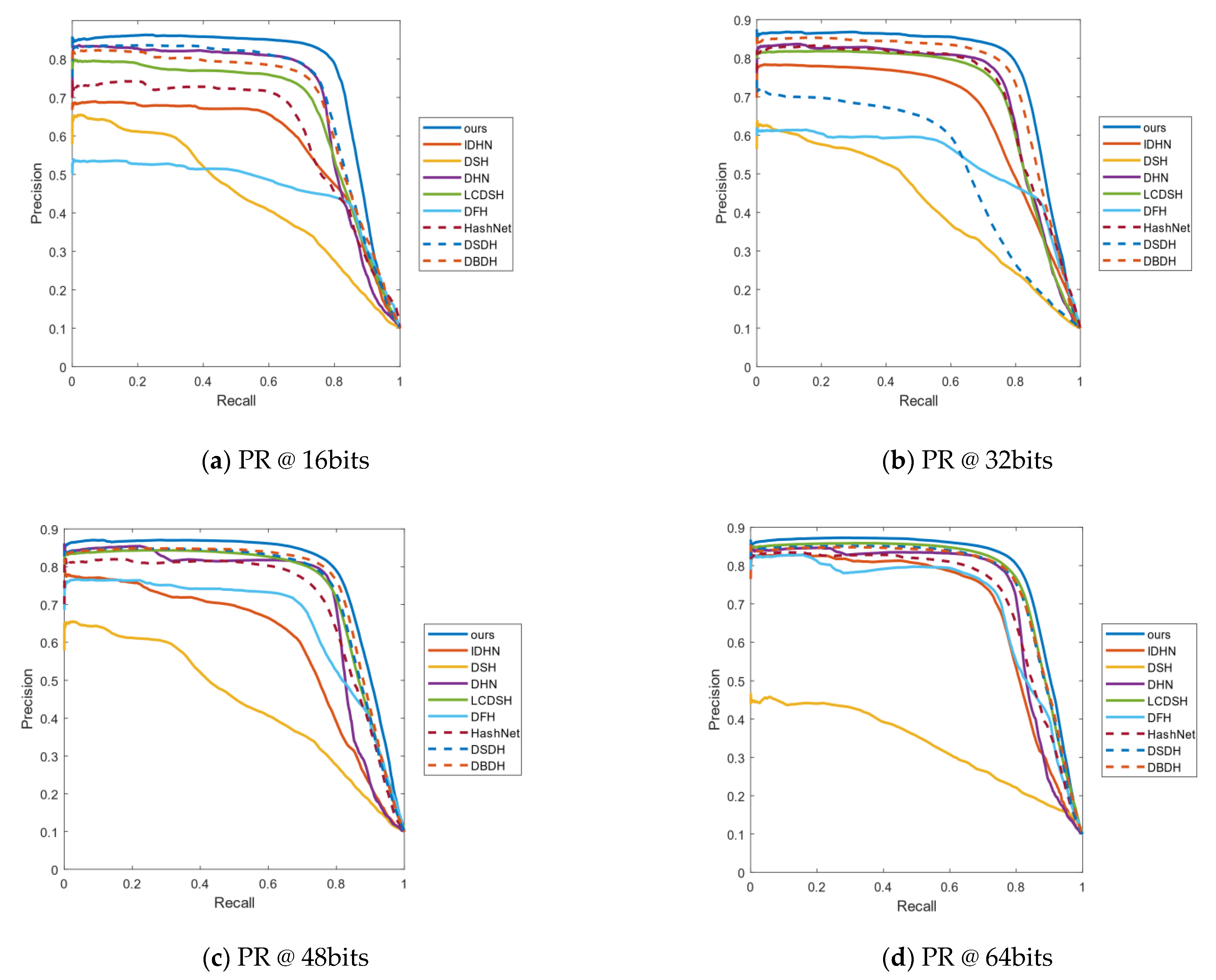
The curve of PR is a significant indicator to access the effect of the model. P represents the precision rate, R the represents recall rate, and PR represents the relationship between the precision rate and recall rate. Generally, recall is set to abscissa and precision is set to ordinate in the PR curves. Figure 3 respectively shows the PR curves of 16, 32, 48 and 64 bits on the CIFAR-10 data set. As can be seen from Figure 3a, the curves of our method are obviously higher than those of the other algorithms. Hence, the area under the PR curve of our method is the largest, which shows that our method has better results than the other methods. Similarly, in Figure 3b,c, our algorithm is higher than DBDH, which has the best performance among all the comparative methods. In Figure 3d of the hash code with length 64, the performance of DHIDA is not as obvious as the other three bits, but the best results are still obtained, compared with other algorithms.

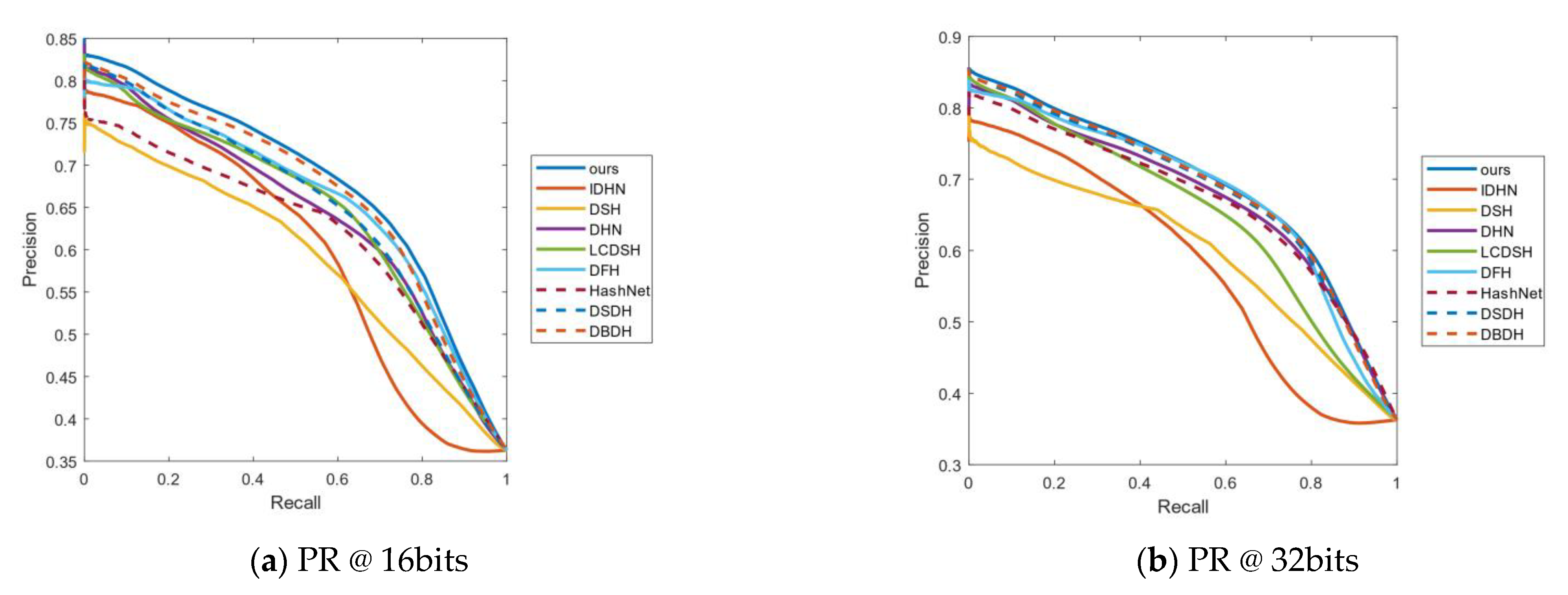
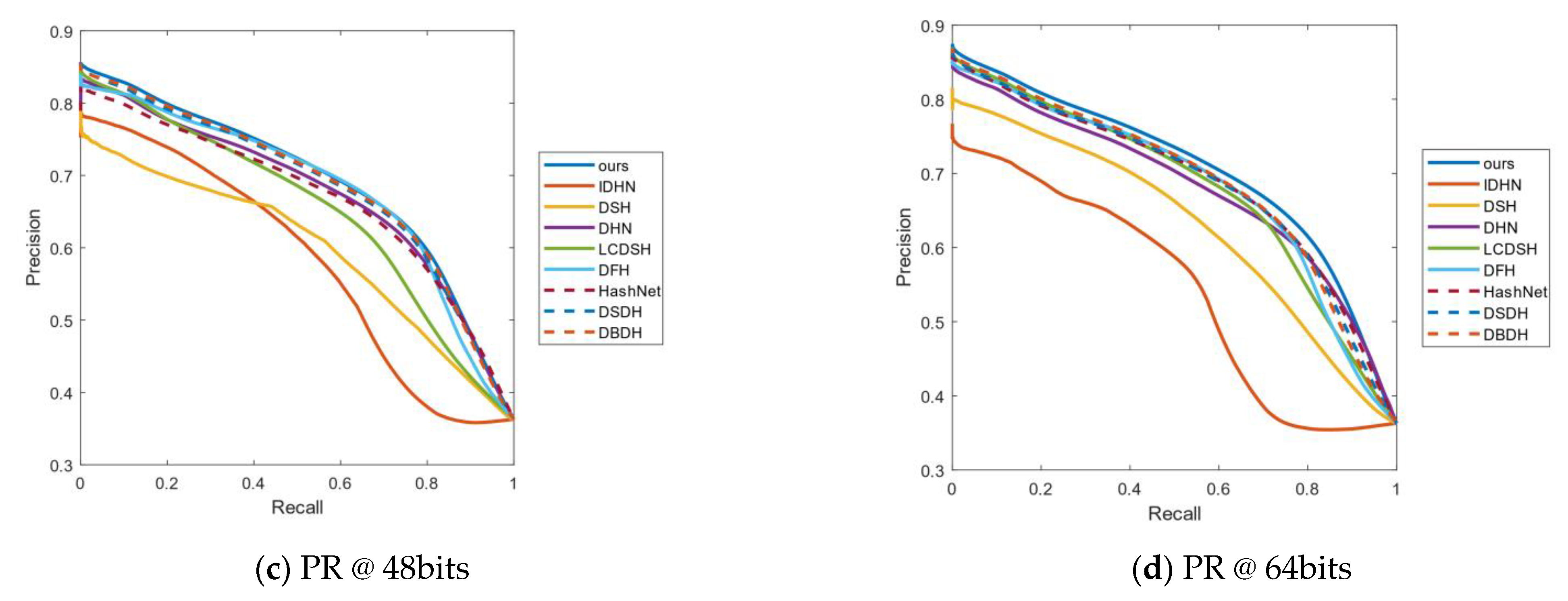
Figure 4 respectively shows the PR curves of 16, 32, 48 and 64 bits on the NUS-WIDE data set. As shown in Figure 4a,d, among all the comparison algorithms, DBDH has the best effect; the PR curve of our method is significantly higher than that of the DBDH method. Therefore, the performance of our model is better than that of the other models. In Figure 4b,c, the PR curves of all the methods are relatively concentrated, but our method still achieves the best performance.

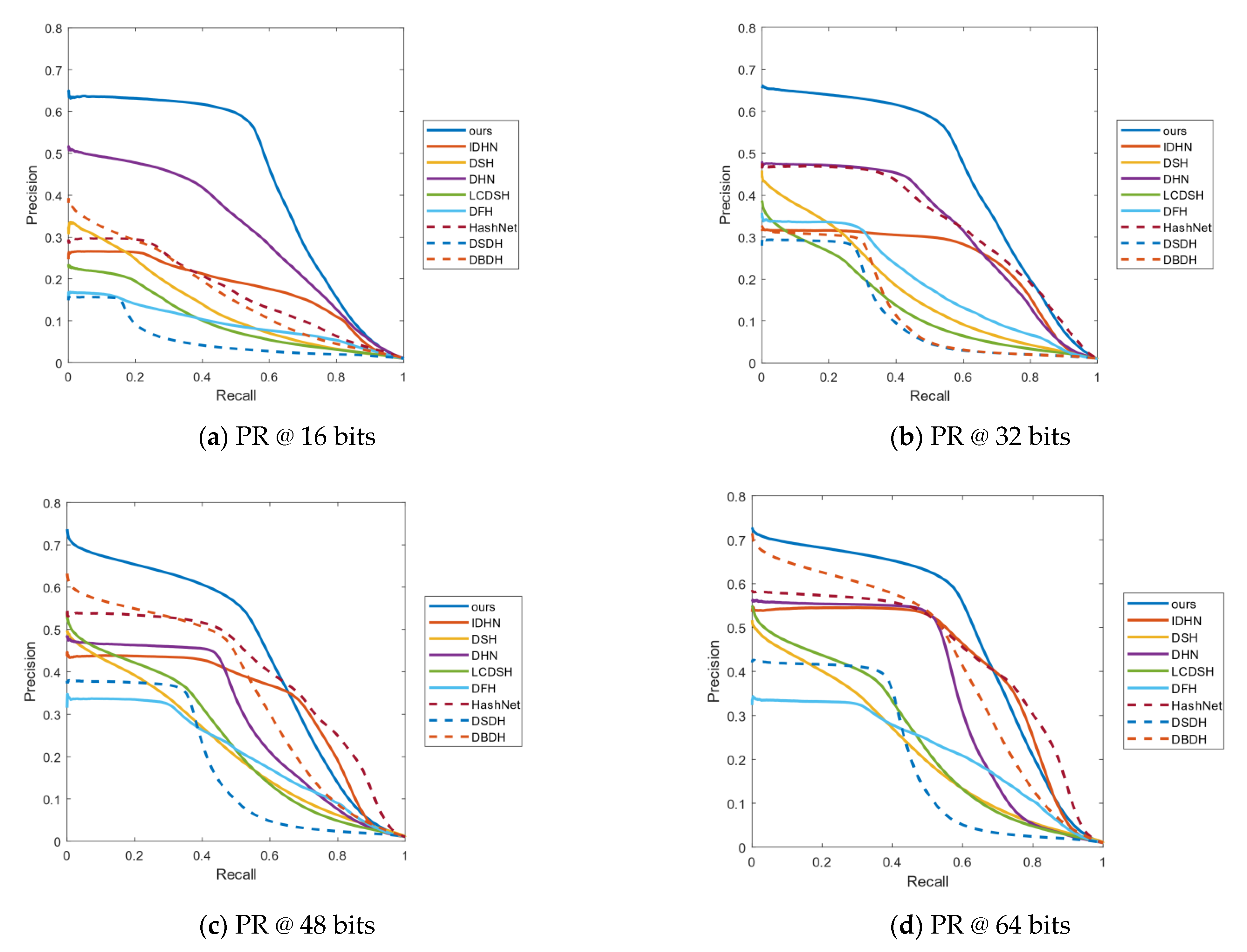
Figure 5 shows the PR curves of 16, 32, 48 and 64 bits on the Imagenet-100 data set. As shown in Figure 5a,b, the area enclosed by our PR curve is the largest, compared to DHN and HashNet. Therefore, the performance of our method is the best when the length of the hash code is 16 bits and 32 bits. In Figure 5c,d, although the PR curve of our method intersects with the PR curve of HashNet and IDHN, it is not difficult to see that the area above the intersection is larger than the area below the intersection, so the performance of our method is still the best among all the compared methods.

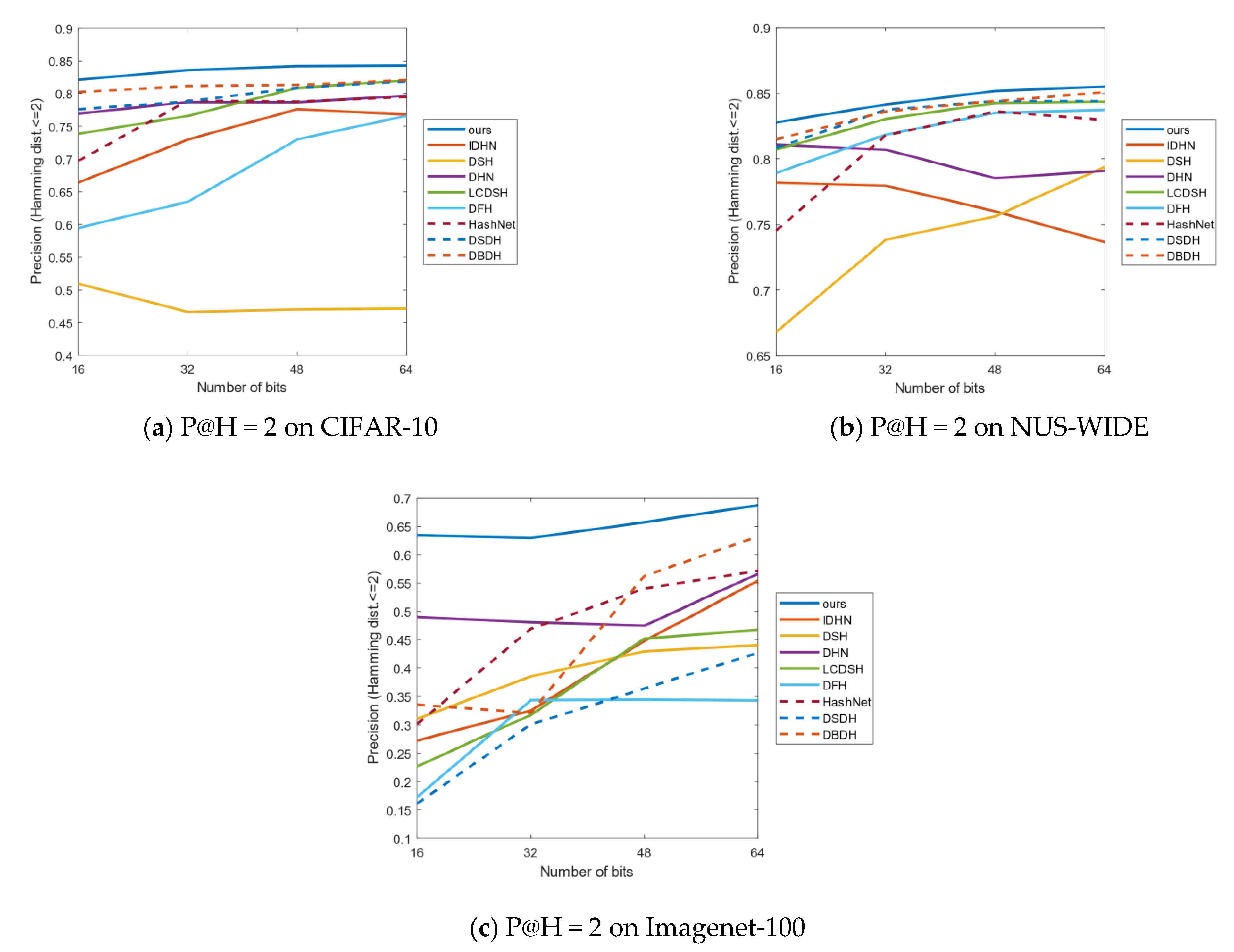
In order to achieve the goal that the Hamming ranking only needs $O\left(1\right)$ time searches, the performance of the P@H = 2 is very significant for the retrieval of the binary space. As shown in Figure 6a–c, comparing the P@H = 2 results of all methods, our method achieves the highest precision on the three data sets, which verifies that our model can be concentrated with more relevant points than all the compared methods. Particularly, P@H = 2 of our method on 64 bits achieves optimal performance on the three data sets.

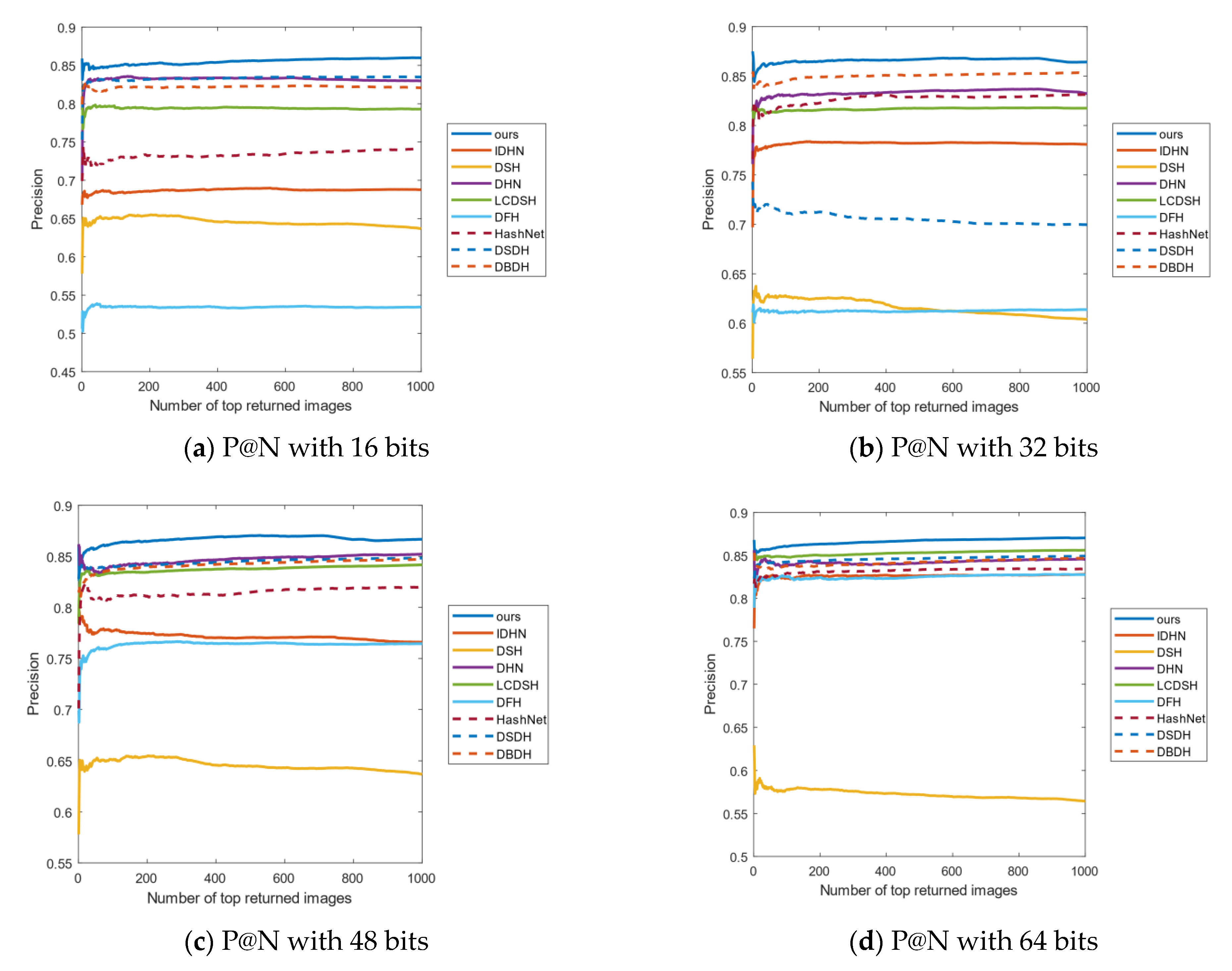
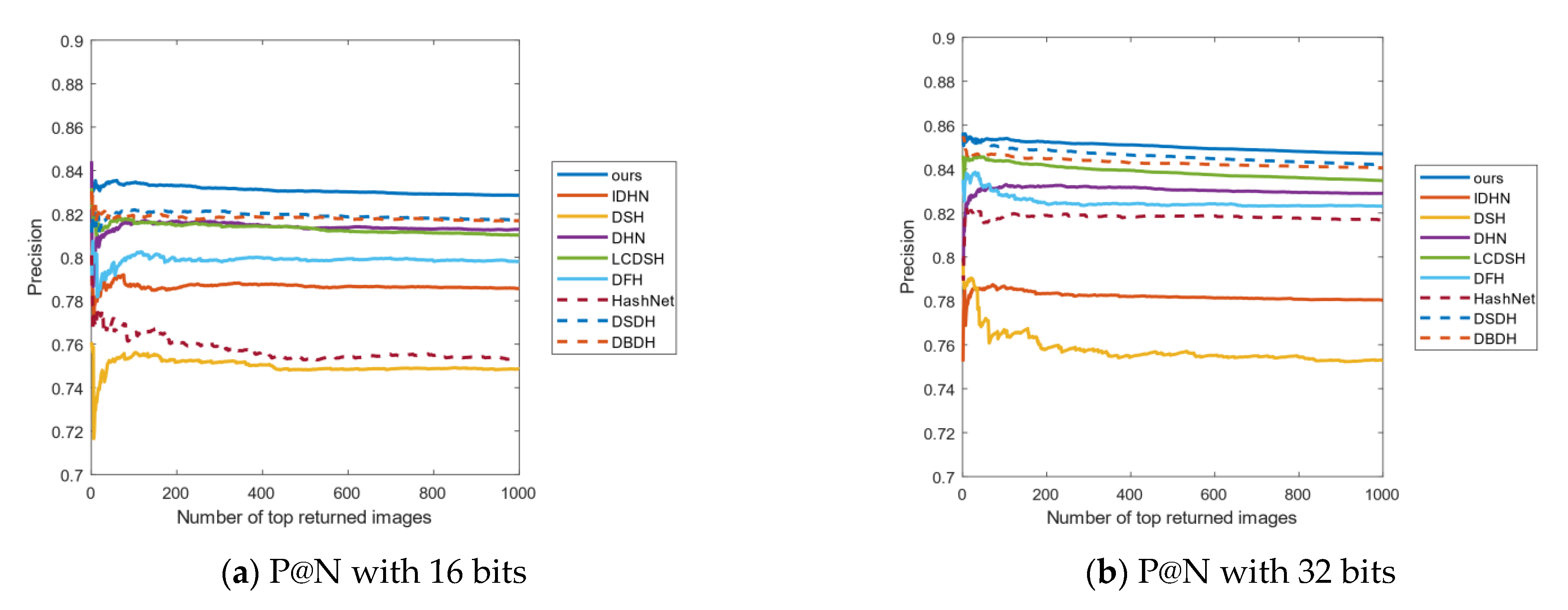
Another important evaluation indicator is the curves of P@N. The experiments choose to return the accuracy of the first 1000 images. Figure 7 shows the P@N results on the CIFAR-10 data set, which shows that our method has achieved better precision than the other methods. For example, in Figure 7a–c, our method returns higher accuracy than the other algorithms. In Figure 7d, the growth of accuracy is slightly lower than the other three bits, but it is still the best compared with other methods. Hence, our method is obtained at a lower recall rate and with a good result, which is very beneficial for an accurate image retrieval system.

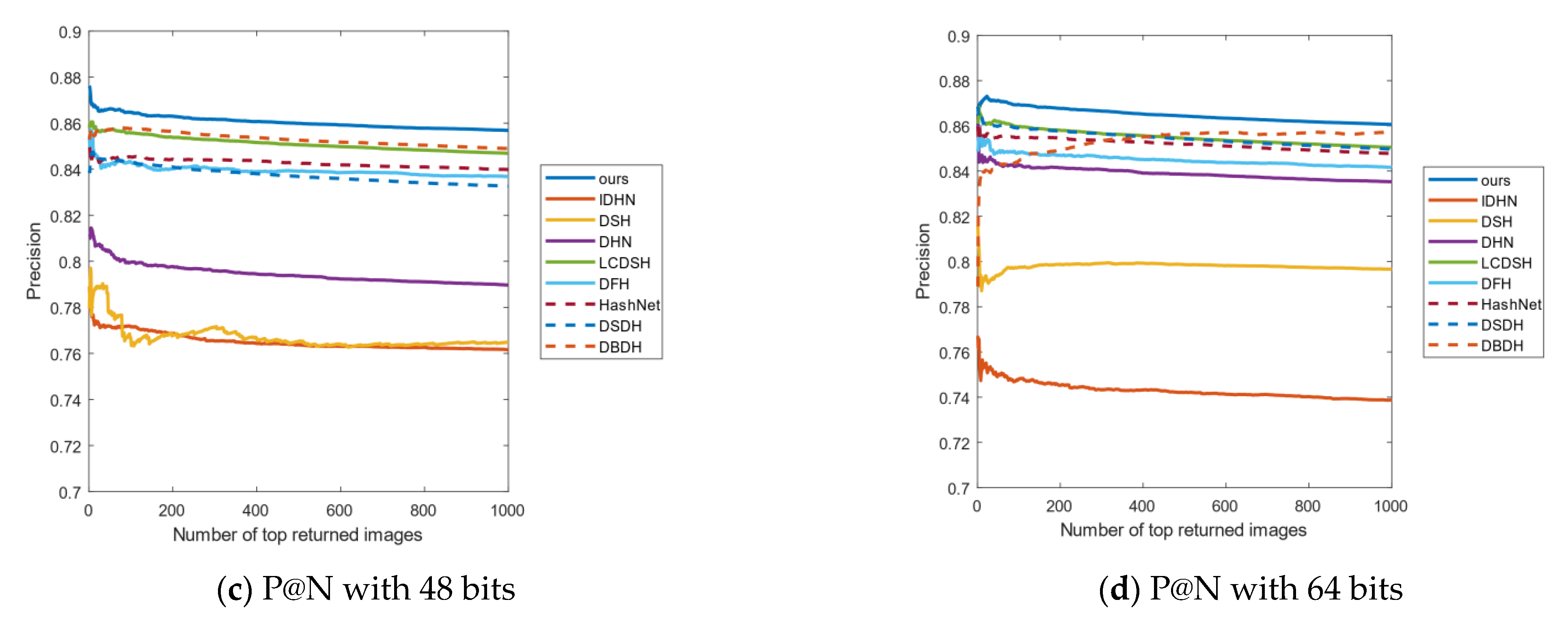
Figure 8 shows the P@N curves on the NUS-WIDE data set. As can be seen from Figure 8a–d, with the increase in the length of the hash code, the accuracy also increases. The accuracy of all methods returning the first 1000 images is relatively stable, and our method has the highest accuracy.

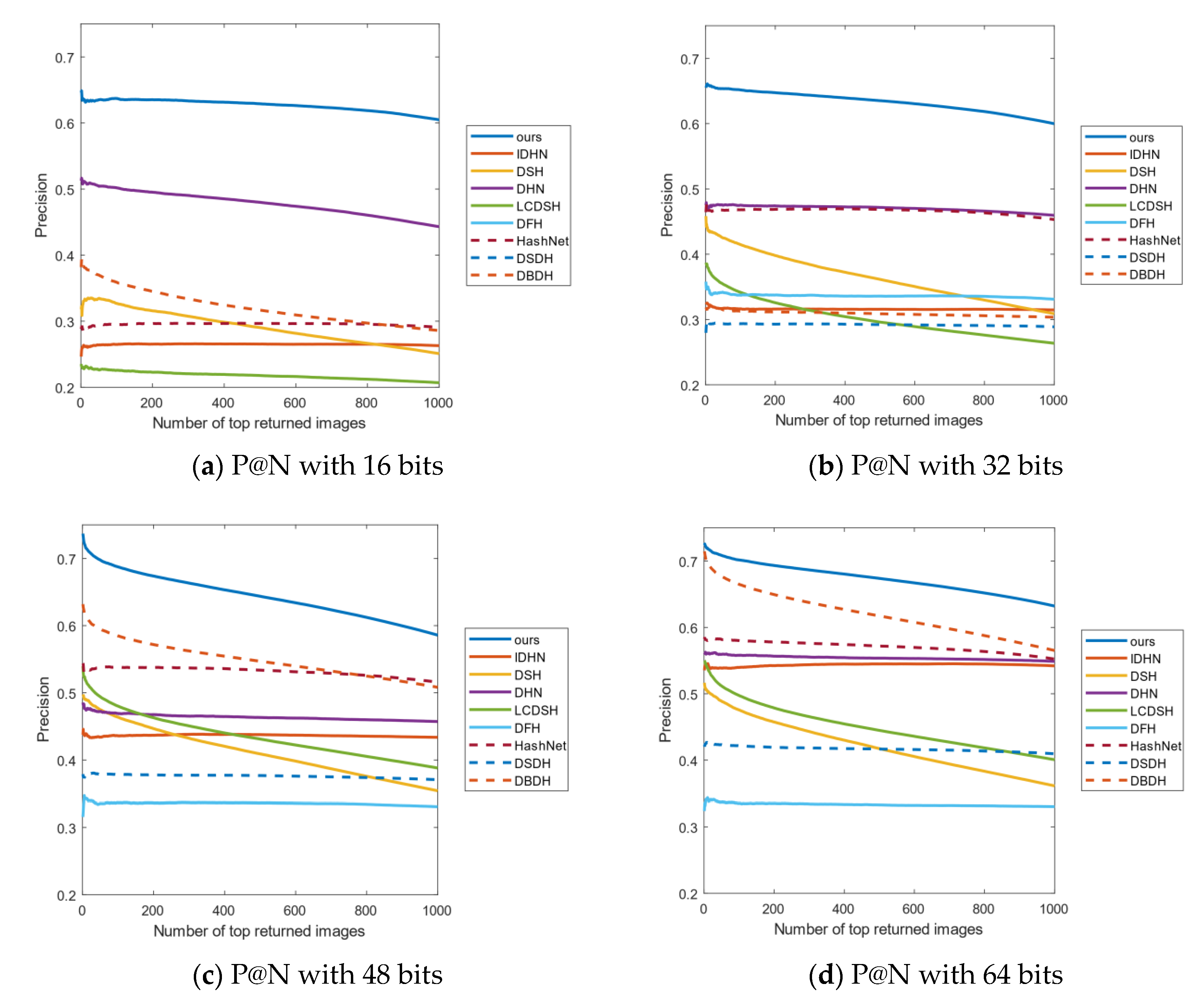
Figure 9 shows the P@N curves on the Imagenet-100 data set. As can be seen from Figure 9a,b, when the length of the hash code is 16 and 32 bits, the accuracy of this method is obviously better than the other methods. Meanwhile, in Figure 9c,d, with the increase in the number of returned images, the corresponding precision of our method decreases in a small range, but the accuracy of our method is still the highest.

4.4. Empirical Analysis

The results of the ablation experiment are shown in

Table 4. Ablation experiments.

	DHIDA-A	DHIDA-I	DHIDA-R	DHIDA-D	DHIDA
Alexnet	√	√
ResNet18			√	√	√
$f\left(\mathit{u}\right)$		√	√	√	√
DANet				√
IDA					√
mAP	0.7240	0.7641	0.8021	0.8076	0.8213

. This study chooses the hash code of length 16 bits to conduct an empirical experiment on the CIFAR-10 data set. The DHIDA-A model represents the algorithm without the attention mechanism on the Alexnet network, and the mAP of the experimental results is 72.40%. The DHIDA-I model indicates that the piecewise function is added to the Alexnet network. At this time, the result of mAP is increased by 4.0%, which proves the validity of the piecewise function. The DHIDA-R model uses the ResNet18 as the backbone network based on DHIDA-I. The experimental result is 80.21%, and the mAP is improved by 3.7%. The DHIDA-D model indicates that the dual attention mechanism is added based on the DHIDA-R architecture, and its mAP is increased by 0.6%. Finally, DHIDA represents the IDA module, is added to the DHIDA-R, and its mAP result is increased by 2.0%, which shows improvement in the IDA module of the optimizing effect on the entire image retrieval system. In addition, √ represents adding the module to the baseline model.

5. Conclusions

Deep hashing for image retrieval is widely used in real applications. However, the existing hashing methods utilizing CNN cannot fully extract image semantic feature information, and there is a lack of correlation between the features. This paper combines the IDA module with the ResNet18 backbone network and proposes a DHIDA model, which effectively overcomes the defect of insufficient and imbalanced feature extraction in shallow networks. In addition, in the process of generating the hash code, this paper designs a new piecewise function to reduce quantization error.

The theoretical analysis and experimental results show that the DHIDA model can improve the accuracy of the hash code. In particular, the value of the mAP increases significantly by 2% when the IDA module is embedded in the network. At the same time, the use of the piecewise function can obviously improve the retrieval accuracy. The effectiveness of the IDA module and piecewise function is further proved by ablation experiments. Furthermore, in the application of the image retrieval system, extensive experiments proved that the performance of the DHIDA model obviously outperforms other hashing methods on the CIFAR-10, NUS-WIDE and ImageNet-100 data sets.

References

- Zhang, Z.; Liu, L.; Shen, F. Binary multi-view clustering. IEEE Trans. Pattern Anal. Mach. Intell. 2018, 41, 1774–1782. [Google Scholar] [CrossRef] [PubMed]
- Pachori, S.; Deshpande, A. Hashing in the zero-shot framework with domain adaptation. Neurocomputing 2018, 275, 2137–2149. [Google Scholar] [CrossRef] [Green Version]
- LeCun, Y.; Bengio, Y.; Hinton, G. Deep learning. Nature 2015, 521, 436–444. [Google Scholar] [CrossRef] [PubMed]
- Lin, K.; Yang, H.F.; Hsiao, J.H. Deep learning of binary hash codes for fast image retrieval. In Proceedings of the IEEE Conference on Computer Vision and Pattern Recognition Workshops, Boston, MA, USA, 7–12 June 2015; pp. 27–35. [Google Scholar]
- Li, W.J.; Wang, S. Feature learning based deep supervised hashing with pairwise labels. arXiv 2015, arXiv:1511.03855. [Google Scholar]
- Huang, L.K.; Chen, J. Accelerate learning of deep hashing with gradient attention. In Proceedings of the IEEE/CVF International Conference on Computer Vision, Seoul, Korea, 27–28 October 2019; pp. 5271–5280. [Google Scholar]
- Yuan, L.; Wang, T. Central similarity quantization for efficient image and video retrieval. In Proceedings of the IEEE/CVF Conference on Computer Vision and Pattern Recognition, Seattle, WA, USA, 16–18 June 2020; pp. 3083–3092. [Google Scholar]
- Lv, N.; Wang, Y. Deep Hashing for Motion Capture Data Retrieval. In Proceedings of the IEEE International Conference on Acoustics, Speech and Signal Processing (ICASSP), Toronto, ON, Canada, 6–11 June 2021; pp. 2215–2219. [Google Scholar]
- Gong, Y.; Lazebnik, S. Iterative quantization: A procrustean approach to learning binary codes for large-scale image retrieval. IEEE Trans. Pattern Anal. Mach. Intell. 2012, 35, 2916–2929. [Google Scholar] [CrossRef] [Green Version]
- Li, P.; Han, L. Hashing nets for hashing: A quantized deep learning to hash framework for remote sensing image retrieval. IEEE Trans. Geosci. Remote Sens. 2020, 58, 7331–7345. [Google Scholar] [CrossRef]
- Zhe, X.; Chen, S. Deep class-wise hashing: Semantics-preserving hashing via class-wise loss. IEEE Trans. Neural Netw. Learn. Syst. 2019, 31, 1681–1695. [Google Scholar] [CrossRef] [Green Version]
- Yan, X.; Zhu, F.; Yu, P.S.; Han, J. Feature-based similarity search in graph structures. ACM Trans. Database Syst. (TODS) 2006, 31, 1418–1453. [Google Scholar] [CrossRef]
- Liu, D.; Shen, J.; Xia, Z.; Sun, X. A content-based image retrieval scheme using an encrypted difference histogram in cloud computing. Information 2017, 8, 96. [Google Scholar] [CrossRef] [Green Version]
- Zheng, L.; Yang, Y. A Decade Survey of Instance Retrieval. IEEE Trans. Pattern Anal. Mach. Intell. 2018, 40, 1224–1244. [Google Scholar] [CrossRef] [Green Version]
- Datar, M.; Immorlica, N. Locality-sensitive hashing scheme based on p-stable distributions. In Proceedings of the Twentieth Annual Symposium on Computational Geometry, Brooklyn, NY, USA, 8–11 June 2004; pp. 253–262. [Google Scholar]
- Yang, H.F.; Lin, K. Supervised learning of semantics-preserving hash via deep convolutional neural networks. IEEE Trans. Pattern Anal. Mach. Intell. 2017, 40, 437–451. [Google Scholar] [CrossRef] [PubMed] [Green Version]
- Liu, H.; Wang, R. Deep supervised hashing for fast image retrieval. In Proceedings of the IEEE Conference on Computer Vision and Pattern Recognition, Las Vegas, NV, USA, 27–30 June 2016; pp. 2064–2072. [Google Scholar]
- Zheng, X.; Zhang, Y. Deep balanced discrete hashing for image retrieval. Neurocomputing 2020, 403, 224–236. [Google Scholar] [CrossRef]
- Wagenpfeil, S.; Engel, F.; Kevitt, P.M.; Hemmje, M. Ai-based semantic multimedia indexing and retrieval for social media on smartphones. Information 2021, 12, 43. [Google Scholar] [CrossRef]
- Li, Q.; Sun, Z. Deep supervised discrete hashing. arXiv 2017, arXiv:1705.10999. [Google Scholar]
- Fan, L.; Ng, K.W. Deep polarized network for supervised learning of accurate binary hashing codes. In Proceedings of the Twenty-Ninth International Joint Conference on Artificial Intelligence (IJCAI-20), Yokohama, Japan, 7–15 January 2020; pp. 825–831. [Google Scholar]
- Wang, J.; Chen, B.; Dai, T.; Xia, S.T. Webly Supervised Deep Attentive Quantization. In Proceedings of the IEEE International Conference on Acoustics, Speech and Signal Processing (ICASSP), Toronto, ON, Canada, 6–11 June 2021; pp. 2250–2254. [Google Scholar]
- Jiang, Q.Y.; Cui, X.; Li, W.J. Deep discrete supervised hashing. IEEE Trans. Image Process. 2018, 27, 5996–6009. [Google Scholar] [CrossRef] [PubMed] [Green Version]
- Yang, Z.; Raymond, O.I. Deep attention-guided hashing. IEEE Access 2019, 7, 11209–11221. [Google Scholar] [CrossRef]
- Fu, J.; Liu, J.; Tian, H. Dual attention network for scene segmentation. In Proceedings of the IEEE/CVF Conference on Computer Vision and Pattern Recognition, Long Beach, CA, USA, 15–20 June 2019; pp. 3146–3154. [Google Scholar]
- Fu, J.; Liu, J.; Jiang, J.; Li, Y.; Bao, Y. Scene segmentation with dual relation-aware attention network. IEEE Trans. Neural Netw. Learn. Syst. 2020, 32, 2547–2560. [Google Scholar] [CrossRef]
- Gong, Y.; Wang, L.; Li, Y. A Discriminative Person Re-Identification Model with Global-Local Attention and Adaptive Weighted Rank List Loss. IEEE Access 2020, 8, 203700–203711. [Google Scholar] [CrossRef]
- Weiss, Y.; Torralba, A. Spectral hashing. NIPS 2008, 1, 4. [Google Scholar]
- Liu, W.; Wang, J.; Kumar, S.; Chang, S.F. Hashing with graphs. In Proceedings of the 28th International Conference on Machine Learning, Bellevue, WA, USA, 28 June–2 July 2011. [Google Scholar]
- Xia, R.; Pan, Y. Supervised hashing for image retrieval via image representation learning. In Proceedings of the AAAI Conference on Artificial Intelligence, Québec City, QC, Canada, 27–31 July 2014; Volume 28. [Google Scholar]
- Lai, H.; Pan, Y. Simultaneous feature learning and hash coding with deep neural networks. In Proceedings of the IEEE Conference on Computer Vision and Pattern Recognition, Boston, MA, USA, 7–12 June 2015; pp. 3270–3278. [Google Scholar]
- Wang, X.; Shi, Y. Deep supervised hashing with triplet labels. In Proceedings of the Asian Conference on Computer Vision, Taipei, Taiwan, 20–24 November 2016; pp. 70–84. [Google Scholar]
- Zhu, H.; Long, M.; Wang, J. Deep hashing network for efficient similarity retrieval. In Proceedings of the AAAI Conference on Artificial Intelligence, Burlingame, CA, USA, 8–12 October 2016; Volume 30. [Google Scholar]
- Cao, Z.; Long, M. Hashnet: Deep learning to hash by continuation. In Proceedings of the IEEE International Conference on Computer Vision, Venice, Italy, 22–29 October 2017; pp. 5608–5617. [Google Scholar]
- Cao, Y.; Long, M. Deep cauchy hashing for hamming space retrieval. In Proceedings of the IEEE Conference on Computer Vision and Pattern Recognition, Salt Lake City, UT, USA, 18–22 June 2018; pp. 1229–1237. [Google Scholar]
- Zhang, Z.; Zou, Q. Improved deep hashing with soft pairwise similarity for multi-label image retrieval. IEEE Trans. Multimed. 2019, 22, 540–553. [Google Scholar] [CrossRef] [Green Version]
- Zhang, Y.; Peng, C. Hierarchical Deep Hashing for Fast Large-Scale Image Retrieval. In Proceedings of the 2020 25th International Conference on Pattern Recognition (ICPR), Milan, Italy, 10–15 January 2021; pp. 3837–3844. [Google Scholar]
- Zhang, H.; Goodfellow, I.; Metaxas, D. Self-attention generative adversarial networks. In Proceedings of the International Conference on Machine Learning (PMLR), Long Beach, CA, USA, 10–15 June 2019; pp. 7354–7363. [Google Scholar]
- Zhu, H.; Gao, S. Locality Constrained Deep Supervised Hashing for Image Retrieval. In Proceedings of the 2017 International Joint Conference on Artificial Intelligence, Melbourne, Australia, 19–25 August 2017; pp. 3567–3573. [Google Scholar]
- Li, Y.; Pei, W. Push for quantization: Deep fisher hashing. arXiv 2019, arXiv:1909.00206. [Google Scholar]
Figure 1.
The overall architecture of the deep hash with the improved dual attention module, which is comprised of three key components: (1) pairs of images are fed into the ResNet18 network to obtain deep feature representations; (2) deep features are fed into the IDA module to obtain fusion features; (3) a hash code layer (fch) is used for transforming the fusion feature into K-dimensional binary code.
Figure 2.
The detail of the IDA module. The upper part highlights the position attention module, and the lower part highlights the channel attention module.
Figure 3.
(a–d) represent the PR curves on CIFAR-10 of all algorithms when the length of the hash code is 16 bits, 32 bits, 48 bits and 64 bits, respectively.
Figure 4.
(a–d) represent the PR curves on NUS-WIDE of all algorithms when the length of the hash code is 16, 32, 48 and 64 bits, respectively.
Figure 5.
(a–d) represent the PR curves on Imagenet-100 of all algorithms when the length of the hash code is 16, 32, 48 and 64 bits, respectively.
Figure 6.
P@H = 2 on three data sets.
Figure 7.
(a–d) represent the P@N curves on CIFAR-10 of all algorithms when the length of the hash code is 16, 32, 48 and 64 bits, respectively.
Figure 8.
(a–d) represent the P@N curves on NUS-WIDE of all algorithms when the length of the hash code is 16, 32, 48 and 64 bits, respectively.
Figure 9.
(a–d) represent the P@N curves on Imagenet-100 of all the algorithms when the length of the hash code is 16, 32, 48 and 64 bits, respectively.