
CANet: A Combined Attention Network for Remote Sensing Image Change Detection


College of Information Science and Engineering, Xinjiang University, Urumqi 830046, China
*
Author to whom correspondence should be addressed.
Information 2021, 12(9), 364; https://0-doi-org.brum.beds.ac.uk/10.3390/info12090364
Submission received: 10 August 2021
/
Revised: 27 August 2021
/
Accepted: 30 August 2021
/
Published: 7 September 2021
Abstract
:Change detection (CD) is one of the essential tasks in remote sensing image processing and analysis. Remote sensing CD is a process of determining and evaluating changes in various surface objects over time. The impressive achievements of deep learning in image processing and computer vision provide an innovative concept for the task of CD. However, existing methods based on deep learning still have problems detecting small changed regions correctly and distinguishing the boundaries of the changed regions. To solve the above shortcomings and improve the efficiency of CD networks, inspired by the fact that an attention mechanism can refine features effectively, we propose an attention-based network for remote sensing CD, which has two important components: an asymmetric convolution block (ACB) and a combined attention mechanism. First, the proposed method extracts the features of bi-temporal images, which contain two parallel encoders with shared weights and structures. Then, the feature maps are fed into the combined attention module to reconstruct the change maps and obtain refined feature maps. The proposed CANet is evaluated on the two publicly available datasets for challenging remote sensing image CD. Extensive empirical results with four popular metrics show that the designed framework yields a robust CD detector with good generalization performance. In the CDD and LEVIR-CD datasets, the F1 values of the CANet are 3.3% and 1.3% higher than those of advanced CD methods, respectively. A quantitative analysis and qualitative comparison indicate that our method outperforms competitive baselines in terms of both effectiveness and robustness.
1. Introduction
Change detection (CD) in remote sensing images is essentially the detection of change information of the ground’s surface at different time phases [1]. The models of CD based on full supervision and semi-supervision [2,3,4] are used in many fields, such as urban planning, land use, coverage, vegetation change, disaster monitoring, map updating, and ecological environment protection. Along with the continuous development and upgrading of remote sensing satellite technology, researchers can obtain high-resolution remote sensing data. Compared with synthetic aperture radar (SAR) images, high-resolution remote sensing images have greater and richer semantic information. Therefore, high-resolution remote sensing images have emerged as an essential statistics supply in the challenging task of CD. Researchers designed networks to extract change maps with abundant information from high-resolution remote sensing images.
A core step of remote sensing image CD is the construction and analysis of difference maps. In traditional networks, the methods of CD are divided into pixel level and object level [5]. The pixel-based methods use pixels as the basis of analysis. The difference maps of multi-temporal remote sensing images are usually obtained by directly comparing corresponding pixel values. However, pixel-level CD methods [6,7] only use the feature information of a single pixel, ignoring the spatial and spectral information of neighboring pixels, which easily leads to “salt and pepper” noise and incomplete expression in the change region. The object-level CD methods synthesize the spatial and spectral characteristics around the pixel, combine the homogeneous pixels to form the object, and then compare the features of spectral, shape, texture, and spatial context neighborhood based on the object [8,9,10]. However, these methods not only have high complexity in feature extraction but also have poor robustness in capturing images.
Deep learning can automatically, and at multiple levels, extract abstract features of complex objects that have been shown to be an effective means of feature learning. In 2012, deep learning methods won first place in the ImageNet Challenge. Since then, CD research based on deep learning has been developing. Models with fully convolutional network (FCN) [11] structures are widely used in remote sensing CD tasks [12,13] to extract better features in pictures. U-Net [14] has achieved certain results in CD. Subsequently, Siamese networks have been used and have become a popular and even standard CD method in this field [15,16,17]. With the continuous innovation of the three networks mentioned above in this field of CD, the CD model is constantly optimized and improved. For example, based on deep belief networking, Gong et al. [18] proposed a creative method of SAR image CD in 2015. In this method, the neural network is trained to generate CD difference maps directly from two images. The process of generating difference maps is omitted to avoid the influence of rough difference maps on CD results. Wang et al. [19] proposed an end-to-end network to deal with high-dimensional problems, which can extract rich information from hyperspectral images. In 2018, the proposed CDNet [12] combined SLAM based on multi-sensor fusion and fast density 3D reconstruction to roughly register image pairs, and then used deep learning methods for pixel-wise CD in street scenes. FC-EF [15] proposes three fully convolutional structures for the CD of registered image pairs. This method uses jump joins to supplement local refinements of spatial details, resulting in accurate boundary change maps that can detect RGB and multispectral images. FC-Siam-diff [15] and FC-Siam-conc [15] are derived from the FC-EF model. FCN-PP [20], an FCN with pyramid pooling, has been proposed for landslide detection. It consists of a U-shaped structure for learning the deep-level features of input images and a pyramid pooling layer for expanding the receptive field. In addition, pyramid pooling can overcome the shortcomings of global pooling. STANet [16] added BAM and PAM attention modules based on the Siamese network to make the CD network have suitable results. CD-UNet++ [21] proposed an end-to-end CNN structure for the CD of high-resolution satellite images and proposed a new UNet++ model, which can achieve deep supervision and capture subtle changes in complex changed scenes. In their method, deep supervision enhances the characterization and identification performance of shallow features. DASNet [17] used an attention mechanism to extract features and obtain better feature representation. In 2021, NestNet [22] proposed an effective remote sensing CD method based on UNet++ [23]. The model can automatically extract features from input images and perform feature fusion on two images from different periods.
There are common problems with the abovementioned CD models. First, continuous down-sampling will cause position information to deviate, which may lead to the missed detection of small targets. Second, the extracted features from the model are usually sensitive to noise, shadow, and other factors due to the lack of features that can clearly distinguish the changed regions from the unchanged regions. Inspired by [16,24], we designed a new CD network architecture. An asymmetric convolution block (ACB) can enhance the robustness of a network model, enable a network to repeatedly extract the features of the central area, as well as increase the weight of the area, and does not introduce a lot of parameters and computation. Simultaneously, ACB improves the sensitivity and accuracy of a CANet by enhancing the activation of features in key areas. In addition, many researchers [25,26,27] note that the combination of spatial attention and channel attention in a certain way not only makes the network pay attention to the areas of interest but also effectively enhances the performance of feature identification. Hence, we propose a combined attention mechanism, including channel attention, position attention, and spatial attention. This mechanism is used to obtain more refined image features to strengthen the performance of the model in identifying changes and improve its ability to recognize pseudo changes. The CANet is characterized by its suitable performance. Experiments on two datasets provided by [16,28] prove the effectiveness of this method. The main contributions of this article are as follows:
We propose a combined attention mechanism, which leverages spatial, channel, and position information to discriminate fine features, so as to obtain rich information of detected objects. The application of this mechanism improves the detection performance of small targets:
- We introduce an asymmetric convolution block (ACB) in our model. It contributes to the robustness of the model against rotation distortion, with a better generalization ability, without introducing additional hyperparameters and inference times;
- We propose a remote sensing image CD network, which is based on the combined attention and ACB. The CANet achieves state-of-the-art performance on widely used benchmarks, and it effectively alleviates the loss in localization information in the deep layers of convolutional networks.
The rest of this article is structured as follows. Section 2 mainly describes the network structure we propose in greater detail. Section 3 introduces datasets, experimental settings, and evaluation indicators. Section 4 precisely analyzes the experimental results. Section 5 is the conclusion and contains directions for future work.
2. Methodology
We introduce the CANet CD network in this section. First, we introduce the specific process of our method. Then, we describe the combined attention module composed of channel attention, spatial attention, and position attention. Finally, we introduce the structure of the ACB.
2.1. Overview
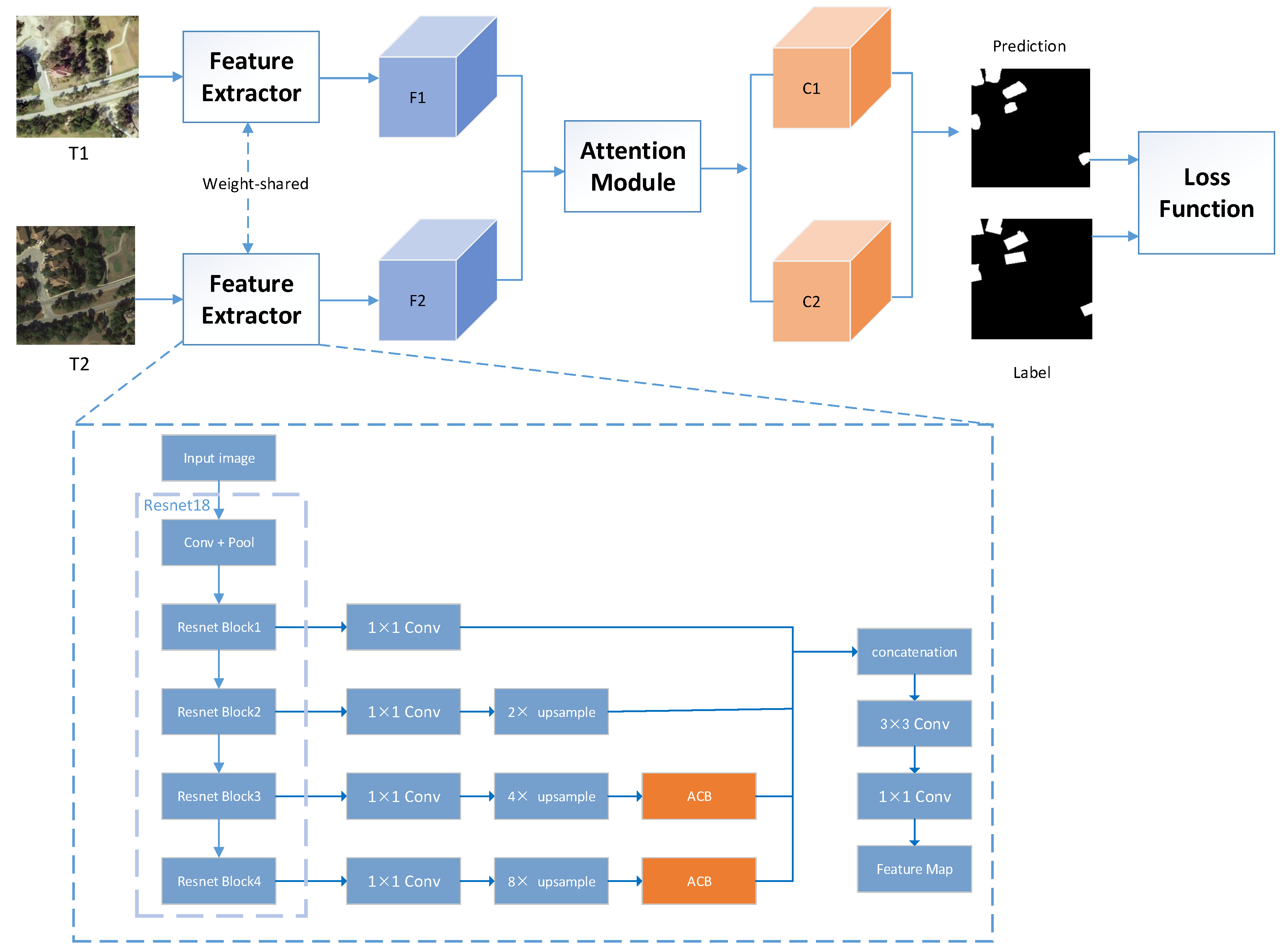
Compared with SAR images, remote sensing images with high-resolution have extensive complex scenes and rich information. Given bi-temporal remote sensing images and , the goal of CD is to generate change maps with the same size as the input images. Using ResNet18 [29] as the backbone network, the bi-temporal satellite images are fed into the Siamese network, and the weights are shared. Next, two rough feature maps of and are obtained. Then, we propose that, through the combined attention mechanism module, two fine feature maps of and are obtained. Ultimately, the final difference maps are calculated by and . In this study, our research object is the binary CD: 1 represents change and 0 represents unchanged.
Our pipeline is shown in Figure 1. In this network, the feature extractor uses ResNet18. The goal of our network is to obtain change maps of the same size as the input. The backbone has five stages, and the receptive field of each stage from top to bottom is reduced by two times to generate different information carried by high-level and low-level values, which helps to generate more accurate feature representations. The specific processing of feature extractor is shown in Table 1 below. We send the output features of four different stages in ResNet18 to the convolution layer, and the channel dimension of feature maps is converted to 96. It aims to give the network an intermediate buffer layer to avoid excessive compression and deformation of the feature maps and retain the feature maps’ information more completely. After the feature maps in the third and fourth stages, we use the ACB. In this model, the ACB module is used to enhance the weight coefficient of the core position of the extracted feature maps. The network can obtain rich feature representation, and the model can obtain better accuracy. Simultaneously, ACB does not bring about super-parameter calculation.
Then, in the channel dimension, the four feature maps are concatenated. In this way, we integrate information at different scales to receive extra distinctive feature maps, including greater deep-level features and more abundant low-level features. The deep-level features have strong semantic information but weak location information, which is not appropriate for small target detection. The features after concatenation are fed into two different convolution layers of and (both strides are 1) to obtain the final feature maps. The two layers generate extra compact and discriminative representations of information by way of digging neighborhood spatial features and decreasing feature channel dimensionality. Then, the generated feature maps are updated by our combined attention module. First, by bilinear interpolation, we adjust the size of the feature maps to be the same as the size of the input images. Then, the distance maps are calculated by the feature distance between the adjusted feature images according to the pixels, , where and are the height and width of the input images, respectively.
In the CD task, the number of changed pixels is quite different from the unchanged pixels. In most cases, the changed pixels occupy a small proportion of the unchanged pixels, which may lead to some deviations in networks during training. To reduce the effect of class imbalance, we use batch-balanced contrastive loss (BCL) in [16] to learn network parameters. Through the proposed network, we obtain distance maps , where represents batch size of the sample, represents the binary label map, 0 represents unchanged, and 1 represents changed. The specific calculation formula is:
In this formula, is set to 2, and subscripts , , and represent batch, height, and width, respectively. Considering the proportion of changed pixels and unchanged pixels, we set to 0.7 in this paper, which will achieve better results. and are the number of unchanged pixel pairs and changed pixel pairs, respectively.
2.2. Combined Attention Module
In the CD, because the specific types of recognition features are also crucial to the identification of changed regions and unchanged regions, studies [30] have shown that extracting features only from simple backbones can cause a large probability of classification errors; thus, extracting a local feature is necessary to use an attention module in CD and enhance feature representation. As shown in Figure 2, inspired by [26,31], we designed a combined attention module. This module strengthens feature extraction in terms of three aspects: spatial, position, and channel. Simultaneously, combined attention enhances the feature representation of feature maps on the original basis. This module is mainly comprised of channel attention, position attention, and spatial attention. In this paper, inspired by [26,31], we designed the combined attention to extract abundant features and capture multi-level features of the channel, both position and spatial. We found that the combined attention mechanism could promote detection performance when all modules were used together. The CANet is very sensitive to the changing edge details of buildings and roads. Simultaneously, the CBAM can capture key fine-grained information.
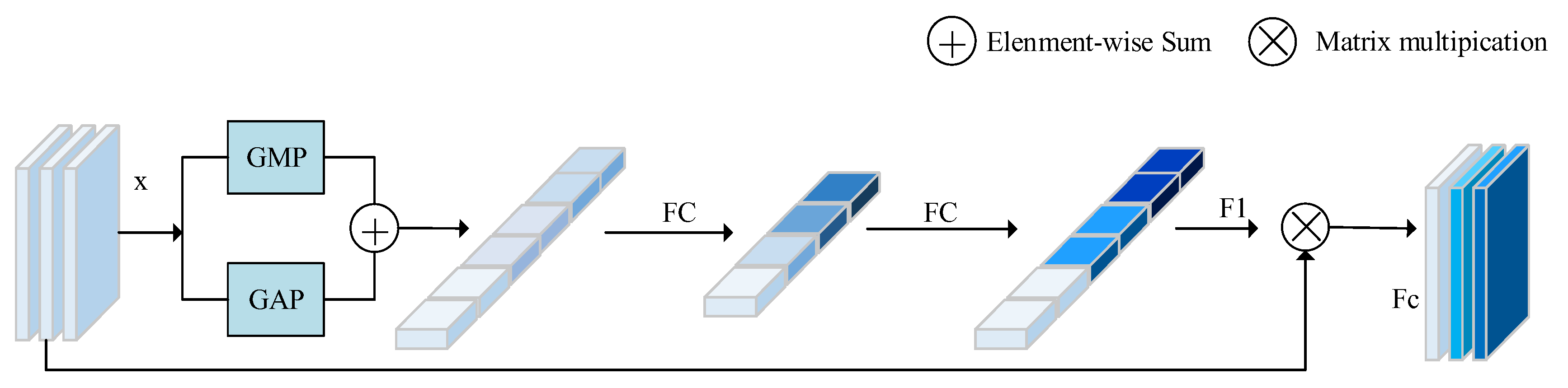
2.2.1. Channel Attention Block
The channel attention block works on the channel scale. The channel attention block selectively emphasizes interrelated channel maps by integrating their relevant features in channel maps. When the feature maps use pooling, the channel attention block processes the input features by employing the parallel pooling of average pooling and maximum pooling, so that less information is lost than in a single pooling. By weighting different channel features, the channel weight in channel attention is different for a feature map. By using the correlation between channels, it can enhance the interdependent feature maps; thus, we use channel attention to construct the relationship between channels in the attention module. The channel attention block first obtains and by the operations of global maximum pooling and global average pooling. The application of global average pooling and global maximum pooling can retain background information and texture features well. Then, feature map is obtained by two full connection layers. Finally, is multiplied by to obtain the final output of . As shown in Figure 3, the specific calculation formula of the module is:
In this formula, and represent the full connection operation, and , where represents the reduction rate and and represent Sigmoid function and ReLU function, respectively.
2.2.2. Spatial Attention Block
In the CANet, spatial attention maps can be generated by using the spatial relationship between features. Unlike channel attention, the spatial attention block pays attention to the spatial dimensions of objects in the feature maps. Based on the original method, we added the operations of maximum pooling and average pooling, where the block is used to manipulate the feature maps along the channel dimension with maximum pooling and average pooling, to highlight information regions. Finally, the spatial attention maps are obtained by a convolution operation. Feature map first goes through the global maximum pooling and global average pooling layers, respectively. The purpose of global average pooling and global maximum pooling is to determine the range and difference part, respectively. Then, we performed concatenation operations on and , and then obtained through and convolution operations, respectively. As shown in Figure 4, the specific calculation formula of the module is:
In this formula, concatenate and first. represents a convolution operation and represents a convolution operation. The and in our method represent the ReLU and the Sigmoid activation function, respectively.
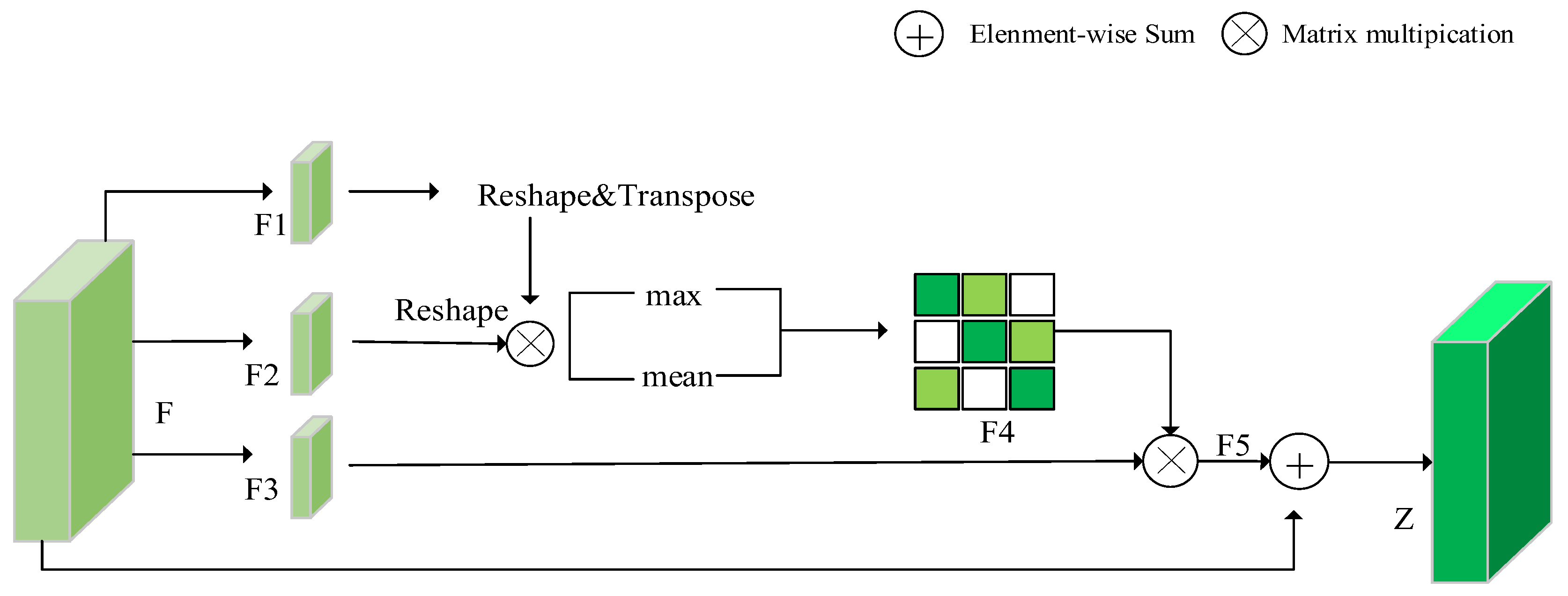
2.2.3. Position Attention Block
As shown in Figure 5, compared with spatial and channel attention blocks, the position attention block shows a suitable representation of the position of each pixel in the input feature maps so as to extract and merge semantically related pixels. This module can capture the spatial dependence between any two positions on the element maps. For the feature of a specific position, the features are updated by the feature aggregation of all locations of the weighted sum, and the weight of the weighted sum is determined by the feature similarity between two locations. That is to say that any two positions with similar features in the feature maps can promote each other, regardless of the distance in the position dimension. The position attention block first obtains after reshaping and other operations for input feature map . The feature maps of and multiply to obtain the matrix, followed by mean and maximum operations. After adding these two branches, is obtained by the Softmax activation function, and is obtained by the matrix multiplication operation between and . Finally, and are added to gain a fine feature map . We can capture and utilize spatial dependence between positions better and learn more useful information through the use of channel attention and position attention in series in our research. The specific formula is as follows:
Among them, is a name of the Softmax function and the matrix multiplication of two tensors is represented by . We use mean function and maximum function to calculate the average value and maximum value of each column of the feature maps and adjust the output size to . More details can be found in [26,27].
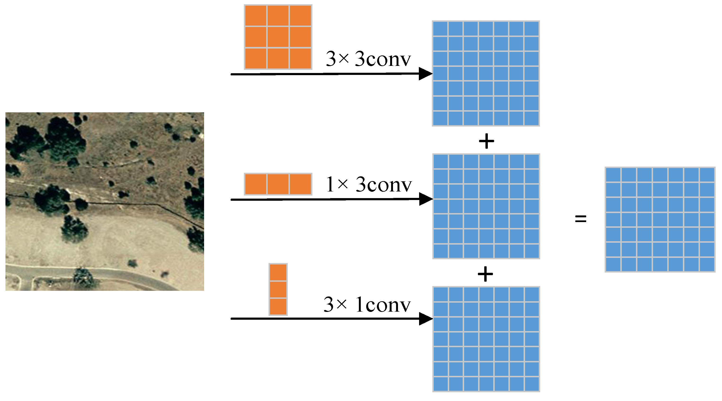
2.3. Asymmetric Convolution Block
Asymmetric convolution is usually used for model compression and acceleration. Previous works have been conducted to directly decompose standard convolutions into and convolutions to reduce the number of parameters; however, studies have found that direct decomposition will lead to inaccurate feature extraction.
Due to the image characteristics of remote sensing CD, inspired by [24], we use ACB to improve network performance to obtain more robust multi-scale features. Our method contains two ACBs from top to bottom, using ACB to enhance the central skeleton part of the squared convolution kernel, thereby enhancing the robustness of remote sensing CD. As the weight proportion of asymmetric convolution in the center cross position is larger, the model can obtain better accuracy. Convolution is the basic part of most networks, and the specific process of ACB is shown in Figure 6. Specifically, convolution in the network is replaced by three convolution layers, including convolution, , and convolution. Eventually, the convolution kernel outputs of the three convolution layers are summed to enrich the feature space. As convolution and convolution are asymmetric, they are also called asymmetric convolution. In addition, ACB does not introduce any hyper-parameters in training and does not require additional parameters or calculations in the inference process.
3. Datasets and Metrics
In our study, we used two high-resolution bi-temporal remote sensing image datasets for training and testing to verify the versatility and performance of our CANet. These two datasets are divided into training, validation, and testing. We adopt two remote sensing image datasets provided by [16,28] to verify our proposed network. Experiments were carried out in [28] to observe the performance of the network in changed objects with seasons, and experiments were carried out by [16] to observe its effect in detecting small and dense building changes.
3.1. Datasets
The first dataset is LEVIR-CD [16], which mainly pays attention to small and dense architectural changes. The LEVIR-CD dataset contains 637 pairs of high-resolution remote sensing images with a resolution of 0.5 m in size of pixels. The date of acquisition varies from 2002 to 2018. These bi-temporal images come from 20 different regions in Texas. Considering the factors such as memory occupation and training speed of the model, we crop the original pixels large-scale remote sensing image pair without overlapping into image pairs. Ultimately, the LEVIR-CD dataset consists of 7120 training image pairs, 1024 validation image pairs, and 2048 test image pairs. The LEVIR-CD is shown in Figure 7a.
The second dataset is CDD [28], which collects the remote sensing images composed of 11 pairs of original images from Google Earth, including 4 pairs of pixels and 7 pairs of pixels for seasonal change remote sensing images. In this dataset, changes in regions due to seasonal variations, illumination, and brightness are not considered significant, such as plants in different seasons. In the CDD dataset, the resolution of bi-temporal images is 3 cm/px to 100 cm/px, with significant seasonal variations. In [32], the original CDD dataset is cut to pixels image pairs by clipping and rotating. Finally, the CDD dataset consists of 10,000 training image pairs, 3000 validation image pairs, and 3000 test image pairs. The CDD is shown in Figure 7b.
3.2. Metrics
Given whether the CANet will achieve better performance, we use precision (P), recall (R), F1, and overall accuracy (OA) as the four evaluation indicators. P represents how many samples in the prediction results are correct. The higher the accuracy is, the smaller the false detection rate is. R represents how many positive samples in the prediction results can be correctly detected. The smaller the recall is, the greater the missed detection rate is. To integrate precision and recall indicators, F1 is proposed. The core idea of F1 is to improve the precision and recall as much as possible while reducing the difference between them. OA represents the ratio between the correct sample and the total sample, i.e., the probability of correct prediction. The specific explanation in the formula is shown in Table 2.
4. Experiment
4.1. Experimental Setting
The proposed method was implemented on PyTorch and trained using a single NVIDIA Tesla V100 graphics processing unit. Our models were fine-tuned on the ImageNet-pre-trained ResNet18 model. Using Adam to optimize the network, was 0.5, was 0.999, and we set the batch size to 16. This method trained a total of 200 epochs. In the first 100 epochs, the initial learning rate was set as 0.001 and the weight linearly decayed to 0 in the remaining 100 epochs. For a fair comparison, the experimental environments (servers, graphics cards, etc.) in which all other SOTA methods were reproduced were identical to those of the methods used in this paper. In addition, for model efficiency comparisons, the batch size of all methods was set to 16 in the training process.
4.2. Results on Different Datasets
In the experiment, this study compared CANet with seven classic CD methods, including CDNet [12], FC-EF [15], FC-Siam-Conc [15], FCN-PP [20], CD-UNet++ [21], STANet [16], and FC-Siam-Diff [15]. The results are shown in Table 3.
We selected several representative CD networks based on deep learning for comparison. Many of these compared networks are improvements on FCN and UNet networks. Their performance data come from [17,33,34] and our experimental results. In this paper, we selected seven models for comparison.
From Table 3, the CANet is the best in four evaluation indicators. The recall, precision, F1, and OA of the CANet are 93.2 %, 93.2%, 93.2%, and 98.4%. This method has achieved good results in remote sensing CD. Compared with seven classic CD methods, the F1 of this method reaches 93.2%, which is 3.3% higher than the method of STANet in Table 3. At the same time, the value of F1 significantly improves compared to other methods in the table. However, the improvement in precision in the four evaluation indicators is the highest, which is 2.8% higher. The experimental data in the table show that the CANet network has robustness.
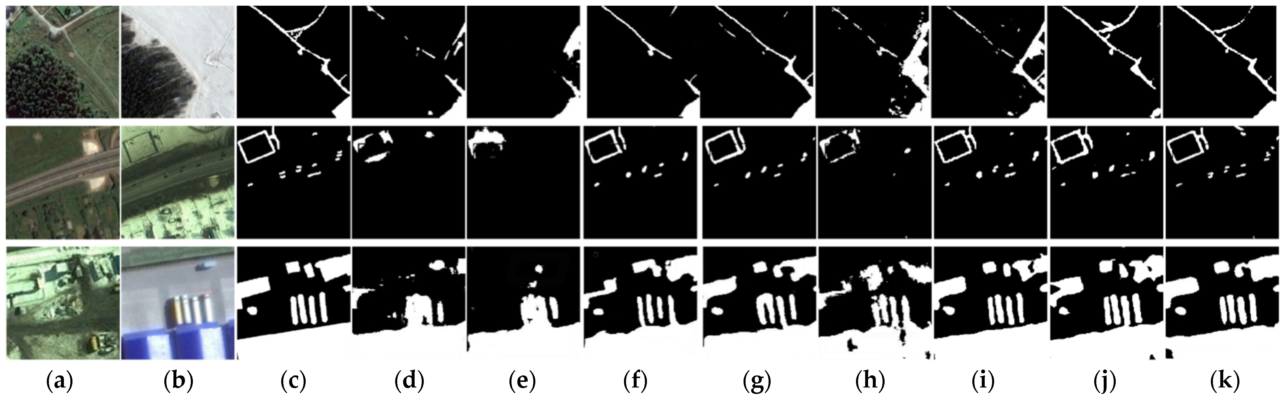
As shown in Figure 8a–k, there are obvious missed detection phenomena in the CDNet and FC-EF models. Many change areas are not detected in the visualization maps, which is different from the label map. The FCN-PP model also missed detection. In CD-UNet++, there is a false detection, which detects some unchanged regions as changed regions. Compared with other models, our proposed CANet detection performance is better. In addition, the change maps obtained by CANet are almost identical to the label maps. Compared to other networks, in all the selected situations, the proposed CANet performs better.
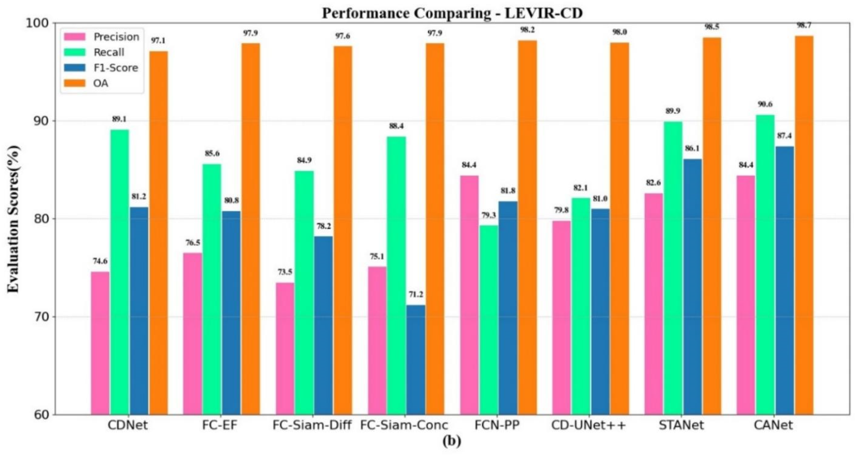
From Table 4, the CANet network based on the combined attention mechanism has good results on four evaluation indexes. Compared with classic detection methods in the table, the CANet has achieved high accuracy in four indicators. The recall, precision, F1, and OA of the CANet are 90.6 %, 84.4%, 87.4%, and 98.7%. Compared with advanced network STANet, the precision and F1 of our method are increased by 1.8% and 1.3%, respectively, which also shows the effectiveness of our method.
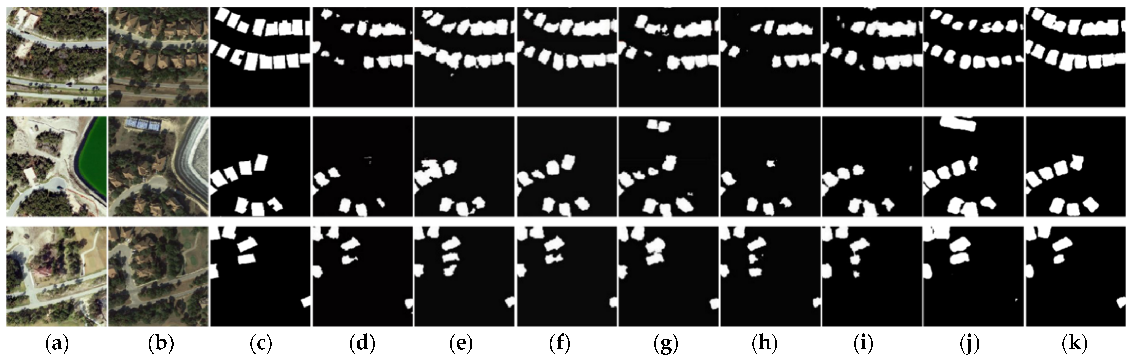
As shown in Figure 9a–k, there are missed detections in CDNet, FC-Siam-conc, and FCN-PP models. Many change areas in the above visualization are not detected, and they are different from the label maps. In CD-Unet++, there are many missed detection problems related to small targets. Through our proposed CANet, problems regarding missed detections and some noises have mainly been solved. Compared to the other networks, in all the selected situations, the proposed CANet performs better.
From Figure 10, the performance of the four indicators of different methods can be compared intuitively. The four indicators of our proposed CANet are much higher than seven classic methods on widely used benchmarks, which shows the superiority of our proposed CANet.
4.3. Accuracy/Efficiency Trade-Offs
To evaluate the efficiency of the model, we choose the CDD dataset to evaluate the space complexity and time complexity of the proposed model.
In this article, we choose the average time cost for each epoch in the training phase and the time cost used throughout the testing phase to represent time complexity; space complexity is represented by the number of parameters of the model. Table 5 lists the time consumption and model parameters of the proposed and compared methods in this paper. The efficiency of the model is expressed in Table 5 by calculating the metric “time/parameter”, where lower values represent better trade-offs between time complexity and space complexity. In addition, the F1 score and OA were chosen to reflect the accuracy of the model because they are more tolerant of data imbalance and provide a better indication of the comprehensive performance of the model. As shown in Table 5, CDNet has the fewest model parameters, but the model’s efficiency is poor and its accuracy is also average. FC-Siam-diff and FC-Siam-conc achieve similar accuracy, but they are inefficient and time consuming. FCN-PP achieves better trade-offs, but its performance is inferior to that of FC-Siam-conc, for example. STANet likewise achieves good trade-offs. The proposed CANet achieves the best trade-offs, i.e., the number of parameters is 11.5 times higher than that of FC-EF, while its time consumption is only 0.3 times that of FC-EF. In addition, the proposed CANet takes only about 322 s to generate the change maps for the entire test set, which equates to an average time of only about 0.11 s to obtain each change map, which is acceptable for most change detection tasks. In summary, the efficiency of CANet is competitive compared to several SOTA methods.
4.4. Ablation Study
To verify that each module we proposed was beneficial to the improvement of network performance, we performed the following ablation experiments on the LEVIR-CD dataset, respectively, as shown in Table 6.
It can be seen that, when training the LEVIR-CD dataset, the combined attention module and ACB are not added to the baseline, and there is a significant gap between the four indicators of the model and the values after the addition of ACB. After the addition of ACB, although the recall value slightly decreases compared with baseline, precision and F1 increase by nearly 2.4% and 1%, respectively, while the value of OA also increases. After adding the combined attention module, compared with the baseline, we can see that precision, OA, and F1 are increased by 6.8%, 0.5%, and 3.5%, respectively. It can be seen from Table 6 that the addition of ACB greatly improves the accuracy of the CANet, while the addition of the combined attention shows the greatest improvement in F1. When ACB and the combined attention module are used simultaneously, the model takes advantage of the spatial, channel, and position information of features to enhance the network robustness, achieving the best results after the balance of four indicators.
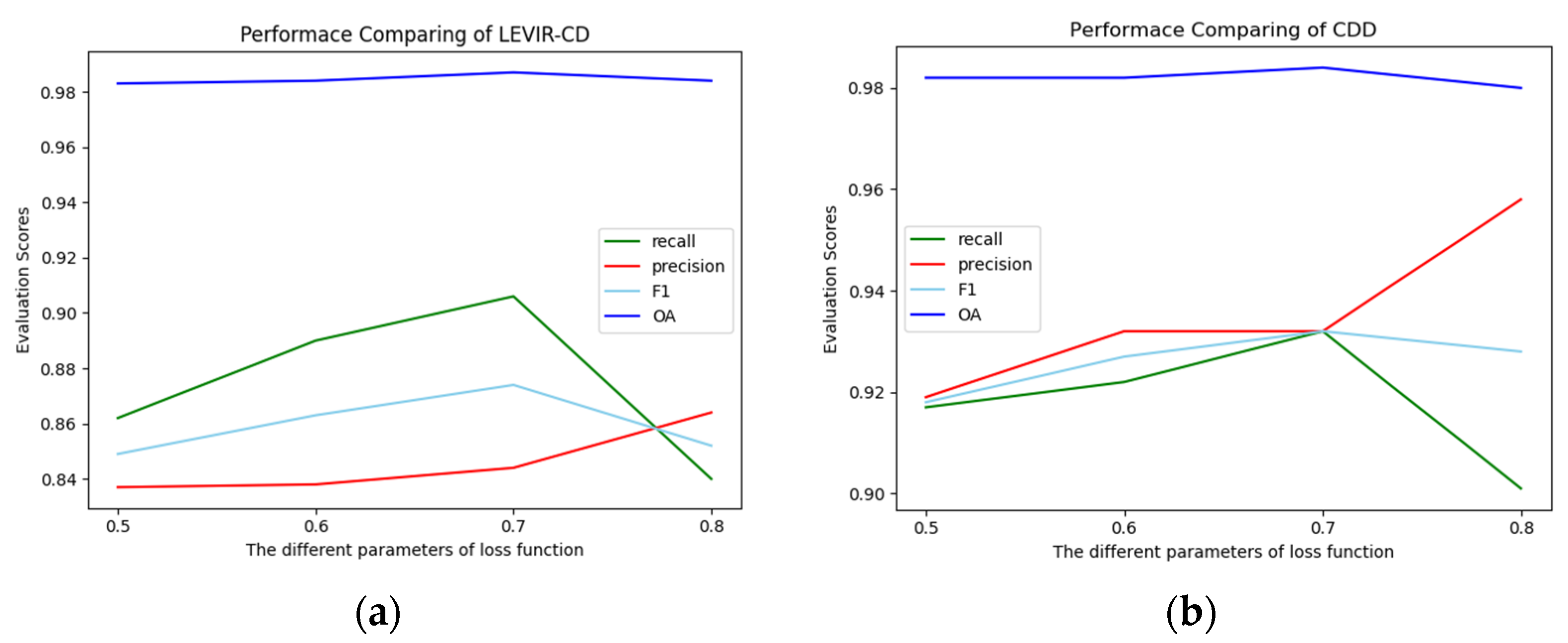
Considering the huge difference in the number of unchanged pixels and changed pixels in the LEVIR-CD and CDD datasets. We set the parameter when using the loss function to update the network by setting the different proportions of unchanged pixels and changed pixels in the loss function calculation. The experimental results are shown in Figure 11a,b. When or , the values of precision, recall, F1, and OA are significantly lower than on datasets of CDD and LEVIR-CD. When , although the precision value is the highest on the two datasets, the values of recall, F1, and OA are all lower than . Comprehensive analysis, when , shows that our proposed model will achieve the best results.
5. Conclusions
In this paper, a remote sensing CD network based on the combined attention mechanism and ACB is proposed. The network integrates different levels of semantic information and uses the combined attention module to better extract the channel, position, and spatial information between features, which also helps to capture more detailed information. In particular, the setting of the combined attention module can reduce memory consumption and improve the robustness of the network. The combined attention module proposed in this paper can be flexibly applied, and can also be used in other CD models to provide new directions. Finally, since the appropriate feature fusion method is adopted and ACB is used to extract the important information in the feature map, the model has achieved excellent results. The effectiveness of the combined attention module and ACB is further proved by ablation experiments. On the CDD dataset, the CANet increases OA, precision, recall, and F1 by 0.8%, 2.8%, 3.9%, and 3.3%, respectively, compared with the STANet model. On the LEVIR-CD dataset, the CANet improves OA, precision, recall, and F1 by 0.2%, 1.8%, 0.7%, and 1.3%, respectively, compared with the STANet model.
In the future, we will be guided by actual demand applications based on remote sensing CD. We will also focus on the study of weakly supervised or unsupervised methods to make the scope of the model’s application wider and focus on the application of semantic changes in real life.
Author Contributions
Conceptualization, D.L.; methodology, S.C.; software, D.L.; validation, A.D., S.C. and D.L.; formal analysis, L.W.; investigation, Y.L.; resource, S.C.; data curation, D.L.; writing—original draft preparation, D.L.; writing—review and editing, L.W.; visualization, D.L. All authors have read and agreed to the published version of the manuscript.
Funding
This research was funded by the Natural Science Foundation of Xinjiang Uygur Autonomous Region grant number 2019D01C033, Tianshan Innovation Team of Xinjiang Uygur Autonomous Region grant number 2020D14044, National Science Foundation of China under grants U1903213, 61771416 and 62041110, the National Key R&D Program of China under grant 2018YFB1403202, and Creative Research Groups of Higher Education of Xinjiang Uygur Autonomous Region under grant XJEDU2017T002.
Data Availability Statement
Publicly available datasets were analyzed in this study. These data can be found here: [https://drive.google.com/file/d/1GX656JqqOyBi_Ef0w65kDGVto-nHrNs9], [https://justchenhao.github.io/LEVIR] (accessed on 28 August).
Conflicts of Interest
The authors declare no conflict of interest.
References
- Singh, A. Review Article Digital change detection techniques using remotely-sensed data. Int. J. Remote Sens. 1989, 10, 989–1003. [Google Scholar] [CrossRef] [Green Version]
- Lv, Z.Y.; Shi, W.; Zhang, X.; Benediktsson, J.A. Landslide Inventory Mapping from Bitemporal High-Resolution Remote Sensing Images Using Change Detection and Multiscale Segmentation. IEEE J. Sel. Top. Appl. Earth Obs. Remote Sens. 2018, 11, 1520–1532. [Google Scholar] [CrossRef]
- Sofina, N.; Ehlers, M. Building Change Detection Using High Resolution Remotely Sensed Data and GIS. IEEE J. Sel. Top. Appl. Earth Obs. Remote Sens. 2017, 9, 3430–3438. [Google Scholar] [CrossRef]
- Coppin, P.; Jonckheere, I.; Nackaerts, K.; Muys, B.; Lambin, E. Digital change detection methods in ecosystem monitoring: A review. Int. J. Remote Sens. 2004, 25, 1565–1596. [Google Scholar] [CrossRef]
- Hussain, M.; Chen, D.; Cheng, A.; Wei, H.; Stanley, D. Change detection from remotely sensed images: From pixel-based to object-based approaches—Sciencedirect. ISPRS J. Photogramm. Remote Sens. 2013, 80, 91–106. [Google Scholar] [CrossRef]
- Wu, C.; Du, B.; Cui, X.; Zhang, L. A post-classification change detection method based on iterative slow feature analysis and bayesian soft fusion. Remote Sens. Environ. 2017, 199, 241–255. [Google Scholar] [CrossRef]
- Deng, J.S.; Wang, K.; Deng, Y.H.; Qi, G.J. Pca-based land-use change detection and analysis using multitemporal and multisensor satellite data. Int. J. Remote Sens. 2008, 29, 4823–4838. [Google Scholar] [CrossRef]
- Volpi, M.; Tuia, D.; Bovolo, F.; Kanevski, M.; Bruzzone, L. Supervised change detection in VHR images using contextual information and support vector machines. Int. J. Appl. Earth Obs. Geoinf. 2013, 20, 77–85. [Google Scholar] [CrossRef]
- Zhang, C.; Li, G.; Cui, W. High-resolution remote sensing image change detection by statistical-object-based method. IEEE J. Sel. Top. Appl. Earth Obs. Remote Sens. 2018, 11, 2440–2447. [Google Scholar] [CrossRef]
- Gil-Yepes, J.L.; Ruiz, L.A.; Recio, J.A.; Balaguer-Beser, A.; Hermosilla, T. Description and validation of a new set of object-based temporal geostatistical features for land-use/land-cover change detection. ISPRS J. Photogramm. Remote Sens. 2016, 121, 77–91. [Google Scholar] [CrossRef]
- Shelhamer, E.; Long, J.; Darrell, T. Fully Convolutional Networks for Semantic Segmentation. IEEE Trans. Pattern Anal. Mach. Intell. 2017, 39, 640–651. [Google Scholar] [CrossRef] [PubMed]
- Alcantarilla, P.F.; Simon, S.; Ros, G.; Roberto, A.; Riccardo, G. Street-view change detection with deconvolutional networks. Auton. Robot. 2018, 42, 1301–1322. [Google Scholar] [CrossRef]
- Papadomanolaki, M.; Verma, S.; Vakalopoulou, M.; Gupta, S.; Karantzalos, K. Detecting urban changes with recurrent neural networks from multitemporal sentinel-2 data. In Proceedings of the IGARSS 2019—2019 IEEE International Geoscience and Remote Sensing Symposium, Yokohama, Japan, 28 July–2 August 2019; pp. 214–217. [Google Scholar]
- Ronneberger, O.; Fischer, P.; Brox, T. U-net: Convolutional networks for biomedical image segmentation. In Proceedings of the International Conference on Medical Image Computing and Computer-Assisted Intervention, Munich, Germany, 5–9 October 2015; Springer: Cham, Switzerland, 2015; pp. 234–241. [Google Scholar]
- Daudt, R.C.; Saux, B.L.; Boulch, A. Fully convolutional siamese networks for change detection. In Proceedings of the 2018 25th IEEE International Conference on Image Processing (ICIP), Athens, Greece, 7–10 October 2018; pp. 4063–4067. [Google Scholar]
- Chen, H.; Shi, Z. A spatial-temporal attention-based method and a new dataset for remote sensing image change detection. Remote Sens. 2020, 12, 1662. [Google Scholar] [CrossRef]
- Chen, J.; Yuan, Z.; Peng, J.; Chen, L.; Li, H. Dasnet: Dual attentive fully convolutional siamese networks for change detection of high resolution satellite images. IEEE J. Sel. Top. Appl. Earth Obs. Remote Sens. 2021, 14, 1194–1206. [Google Scholar] [CrossRef]
- Gong, M.; Zhao, J.; Liu, J.; Miao, Q.; Jiao, L. Change Detection in Synthetic Aperture Radar Images Based on Deep Neural Networks. IEEE Trans. Neural Netw. Learn. Syst. 2016, 27, 125–138. [Google Scholar] [CrossRef]
- Wang, Q.; Yuan, Z.; Du, Q.; Li, X. Getnet: A general end-to-end 2-d cnn framework for hyperspectral image change detection. IEEE Trans. Geosci. Remote Sens. 2019, 57, 3–13. [Google Scholar] [CrossRef] [Green Version]
- Lei, T.; Zhang, Y.; Lv, Z.; Li, S.; Liu, S.; Nandi, A.K. Landslide inventory mapping from bitemporal images using deep convolutional neural networks. IEEE Geosci. Remote Sens. Lett. 2019, 16, 982–986. [Google Scholar] [CrossRef]
- Peng, D.; Zhang, Y.; Guan, H. End-to-End Change Detection for High Resolution Satellite Images Using Improved UNet++. Remote Sens. 2019, 11, 1382. [Google Scholar] [CrossRef] [Green Version]
- Yu, X.; Fan, J.; Chen, J.; Zhang, P.; Han, L. Nestnet: A multiscale convolutional neural network for remote sensing image change detection. Int. J. Remote Sens. 2021, 42, 4902–4925. [Google Scholar] [CrossRef]
- Zhou, Z.; Siddiquee, M.M.R.; Tajbakhsh, N.; Liang, J. Unet++: A nested u-net architecture for medical image segmentation. In Proceedings of the 4th International Workshop on Deep Learning in Medical Image Analysis, Granada, Spain, 20 September 2018; pp. 3–11. [Google Scholar]
- Ding, X.; Guo, Y.; Ding, G.; Han, J. ACNet: Strengthening the kernel skeletons for powerful CNN via asymmetric convolution blocks. In Proceedings of the 2019 IEEE/CVF International Conference on Computer Vision (ICCV), Seoul, Korea, 27 October–2 November 2019; pp. 1911–1920. [Google Scholar]
- Long, C.; Zhang, H.; Xiao, J.; Nie, L.; Chua, T.S. SCA-CNN: Spatial and channel-wise attention in convolutional metworks for image captioning. In Proceedings of the 2017 IEEE Conference on Computer Vision and Pattern Recognition (CVPR), Honolulu, HI, USA, 21–26 July 2017; pp. 6298–6306. [Google Scholar]
- Woo, S.; Park, J.; Lee, J.Y.; Kweon, I.S. CBAM: Convolutional block attention module. In European Conference on Computer Vision (ECCV); Springer: Cham, Switzerland, 2018; pp. 3–19. [Google Scholar]
- Fu, J.; Liu, J.; Tian, H.; Li, Y.; Bao, Y.; Fang, Z. Dual attention network for scene segmentation. In Proceedings of the 2019 IEEE/CVF Conference on Computer Vision and Pattern Recognition (CVPR), Long Beach, CA, USA, 15–20 June 2019; pp. 3141–3149. [Google Scholar]
- Lebedev, M.A.; Vizilter, Y.V.; Vygolov, O.V.; Knyaz, V.A.; Rubis, A.Y. Change Detection in Remote Sensing Images Using Conditional Adversarial Networks. Int. Arch. Photogramm. Remote Sens. Spat. Inf. Sci. 2018, XLII-2, 565–571. [Google Scholar] [CrossRef] [Green Version]
- He, K.; Zhang, X.; Ren, S.; Sun, J. Deep residual learning for image recognition. In Proceedings of the 2016 IEEE Conference on Computer Vision and Pattern Recognition (CVPR), Las Vegas, NV, USA, 27–30 June 2016; pp. 770–778. [Google Scholar]
- Peng, C.; Zhang, X.; Yu, G.; Luo, G.; Sun, J. Large kernel matters—Improve semantic segmentation by global convolutional network. In Proceedings of the 2017 IEEE Conference on Computer Vision and Pattern Recognition (CVPR), Honolulu, HI, USA, 21–26 July 2017; pp. 1743–1751. [Google Scholar]
- Chen, T.; Ding, S.; Xie, J.; Yuan, Y.; Chen, W.; Yang, Y.; Chen, W.; Yang, Y.; Ren, Z.; Wang, Z. ABD-Net: Attentive but diverse person re-identification. In Proceedings of the 2019 IEEE/CVF International Conference on Computer Vision (ICCV), Seoul, Korea, 27 October–2 November 2019; pp. 8350–8360. [Google Scholar]
- Ji, S.; Wei, S.; Lu, M. Fully convolutional networks for multisource building extraction from an open aerial and satellite imagery data set. IEEE Trans. Geosci. Remote Sens. 2019, 57, 574–586. [Google Scholar] [CrossRef]
- Zhang, X.; Yue, Y.; Gao, W.; Yun, S.; Zhang, Y. Difunet++: A satellite images change detection network based on unet++ and differential pyramid. IEEE Geosci. Remote Sens. Lett. 2021. [Google Scholar] [CrossRef]
- Zhi, Z.A.; Yi, W.A.; Yz, A.; Sx, A.; Dpb, C.; Bz, A. CLNet: Cross-layer convolutional neural network for change detection in optical remote sensing imagery. ISPRS J. Photogramm. Remote Sens. 2021, 175, 247–267. [Google Scholar]
Figure 1.
Framework of the CANet network.

Figure 2.
The structure of combined attention mechanism.

Figure 3.
Channel attention block.

Figure 4.
Spatial attention block.

Figure 5.
Position attention block.

Figure 6.
The structure of ACB.

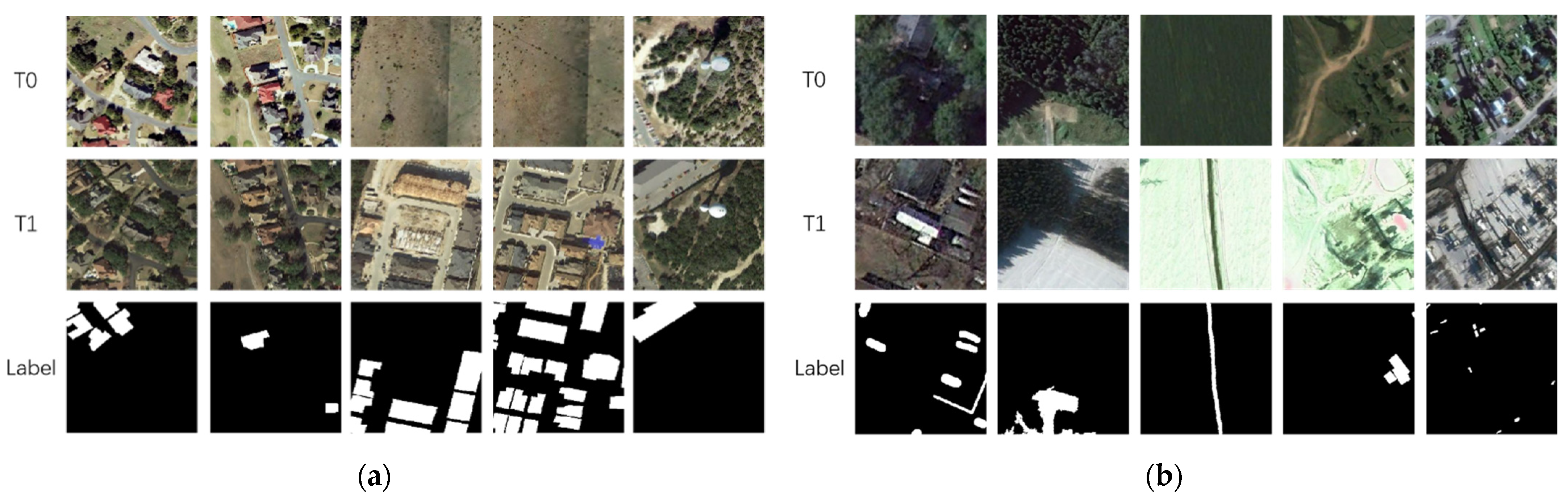
Figure 7.
T0 is change before images, T1 is change after images, and Label represents the changed areas and the unchanged areas: (a) multitemporal remote sensing images from LEVIR-CD dataset; (b) multitemporal remote sensing images from CDD dataset.
Figure 7.
T0 is change before images, T1 is change after images, and Label represents the changed areas and the unchanged areas: (a) multitemporal remote sensing images from LEVIR-CD dataset; (b) multitemporal remote sensing images from CDD dataset.

Figure 8.
Visualization of eight different methods of CDD dataset: (a) represents T1 images; (b) represents T2 images; (c) label; (d) are results obtained by CDNet; (e) are results obtained by FC-EF; (f) are results obtained by FC-Siam-diff; (g) are results obtained by FC-Siam-conc; (h) are results obtained by FCN-PP; (i) are results obtained by CD-UNet++; (j) are results obtained by STANet; (k) are results obtained by CANet.

Figure 9.
Visualization of eight different methods of LEVIR-CD dataset: (a) represents T1 images; (b) represents T2 images; (c) label; (d) are results obtained by CDNet; (e) are results obtained by FC-EF; (f) are results obtained by FC-Siam-diff; (g) are results obtained by FC-Siam-conc; (h) are results obtained by FCN-PP; (i) are results obtained by CD-UNet++; (j) are results obtained by STANet; (k) are results obtained by CANet.

Figure 10.
The performance of different models: (a) the evaluation scores of CDD dataset; (b) the evaluation scores of LEVIR-CD dataset.
Figure 10.
The performance of different models: (a) the evaluation scores of CDD dataset; (b) the evaluation scores of LEVIR-CD dataset.


Figure 11.
The influence of loss function parameters on the model: (a) experiment on the LEVIR-CD; (b) experiment on the CDD.
Figure 11.
The influence of loss function parameters on the model: (a) experiment on the LEVIR-CD; (b) experiment on the CDD.


Table 1.
Operation of backbone.
| Layers | Operation | Input | Output |
|---|---|---|---|
| Conv + Pool | {k = (7,7), s = (2,2), p = (3,3), BN, ReLU} | 3 × 256 × 256 | 64 × 64 × 64 |
| maxpool {k = (3,3), s = (2,2), p = (1,1)} | |||
| Resnet Block1 | {k = (3,3), s = (1,1), p = (1,1), BN} × 4 | 64 × 64 × 64 | 64 × 64 × 64 |
| Resnet Block2 | {k = (3,3), s = (2,2), p = (1,1), BN, ReLU} | 64 × 64 × 64 | 128 × 32 × 32 |
| {k = (3,3), s = (1,1), p = (1,1), BN} × 3 | |||
| Resnet Block3 | {k = (3,3), s = (2,2), p = (1,1), ReLU} | 128 × 32 × 32 | 256 × 16 × 16 |
| {k = (3,3), s = (1,1), p = (1,1), BN} × 3 | |||
| Resnet Block4 | {k = (3,3), s = (2,2), p = (1,1), BN, ReLU} | 256 × 16 × 16 | 512 × 8 × 8 |
| {k = (3,3), s = (1,1), p = (1,1), BN} × 3 |
k represents kernel size; s represents stride; p represents pool.
Table 2.
The detailed explanation of TN, TP, FN, and FP.
| True Value | Predicted Value | |
|---|---|---|
| Positive | Negative | |
| positive | TP | FN |
| negative | FP | TN |
Table 3.
Comparison of CDD dataset results (the best performance is emphasized in bold).
| Method | Rec (%) | Pre (%) | F1 (%) | OA (%) |
|---|---|---|---|---|
| CDNet | 81.7 | 82.7 | 82.2 | 96.4 |
| FC-EF | 76.1 | 81.5 | 77.1 | 94.1 |
| FC-Siam-Diff | 83.6 | 85.8 | 83.7 | 95.8 |
| FC-Siam-Conc | 82.5 | 84.4 | 82.5 | 95.7 |
| FCN-PP | 87.1 | 82.6 | 80.5 | 95.4 |
| CD-UNet++ | 85.9 | 87.6 | 86.8 | 96.7 |
| STANet | 89.3 | 90.4 | 89.9 | 97.6 |
| CANet | 93.2 | 93.2 | 93.2 | 98.4 |
Table 4.
Comparison of LEVIR-CD dataset results. (The best performance is emphasized in bold).
| Method | Rec (%) | Pre (%) | F1 (%) | OA (%) |
|---|---|---|---|---|
| CDNet | 89.1 | 74.6 | 81.2 | 97.1 |
| FC-EF | 85.6 | 76.5 | 80.8 | 97.9 |
| FC-Siam-Diff | 84.9 | 73.5 | 78.2 | 97.6 |
| FC-Siam-Conc | 88.4 | 75.1 | 71.2 | 97.9 |
| FCN-PP | 79.3 | 84.4 | 81.8 | 98.2 |
| CD-UNet++ | 82.1 | 79.8 | 81.0 | 98.0 |
| STANet | 89.9 | 82.6 | 86.1 | 98.5 |
| CANet | 90.6 | 84.4 | 87.4 | 98.7 |
Table 5.
Performance and speed trade-offs. (The best performance is emphasized in bold).
| Method | Train | Test | ||||
|---|---|---|---|---|---|---|
| F1 (%) | OA (%) | T/E | Parameter | Test Time (3000 Images) | ||
| CDNet | 82.2 | 96.4 | ~1879 s | ~1.28 M | 14.68 | ~1020 s |
| FC-EF | 77.1 | 94.1 | ~978 s | ~1.47 M | 6.65 | ~253 s |
| FC-Siam-Diff | 83.7 | 95.8 | ~1134 s | ~1.51 M | 7.51 | ~287 s |
| FC-Siam-Conc | 82.5 | 95.7 | ~1207 s | ~1.62 M | 7.45 | ~288 s |
| FCN-PP | 80.5 | 95.4 | ~1226 s | ~10.02 M | 1.22 | ~149 s |
| CD-UNet++ | 86.8 | 96.7 | ~4637 s | ~9.13 M | 5.07 | ~152 s |
| STANet | 89.9 | 97.6 | ~564 s | ~16.93 M | 0.33 | ~576 s |
| CANet | 93.2 | 98.4 | ~302 s | ~17.03 M | 0.18 | ~322 s |
T/E represents time/epoch; T/E represents time/parameters.
Table 6.
LEVIR-CD dataset ablation experiment (the best performance is emphasized in bold).
| Method | Rec (%) | Pre (%) | F1 (%) | OA (%) |
|---|---|---|---|---|
| baseline | 89.5 | 77.1 | 82.9 | 98.1 |
| +ACB | 88.9 | 79.5 | 83.9 | 98.3 |
| +attention | 89.1 | 83.9 | 86.4 | 98.6 |
| CANet | 90.6 | 84.4 | 87.4 | 98.7 |
Publisher’s Note: MDPI stays neutral with regard to jurisdictional claims in published maps and institutional affiliations. |
© 2021 by the authors. Licensee MDPI, Basel, Switzerland. This article is an open access article distributed under the terms and conditions of the Creative Commons Attribution (CC BY) license (https://creativecommons.org/licenses/by/4.0/).
Share and Cite
MDPI and ACS Style
Lu, D.; Wang, L.; Cheng, S.; Li, Y.; Du, A. CANet: A Combined Attention Network for Remote Sensing Image Change Detection. Information 2021, 12, 364. https://0-doi-org.brum.beds.ac.uk/10.3390/info12090364
AMA Style
Lu D, Wang L, Cheng S, Li Y, Du A. CANet: A Combined Attention Network for Remote Sensing Image Change Detection. Information. 2021; 12(9):364. https://0-doi-org.brum.beds.ac.uk/10.3390/info12090364
Chicago/Turabian StyleLu, Di, Liejun Wang, Shuli Cheng, Yongming Li, and Anyu Du. 2021. "CANet: A Combined Attention Network for Remote Sensing Image Change Detection" Information 12, no. 9: 364. https://0-doi-org.brum.beds.ac.uk/10.3390/info12090364
Note that from the first issue of 2016, this journal uses article numbers instead of page numbers. See further details here.