
Three-Dimensional LiDAR Decoder Design for Autonomous Vehicles in Smart Cities


1
Department of Electronic Engineering, National Taipei University of Technology, Taipei 10608, Taiwan
2
Wistron Corporation, Taipei 11469, Taiwan
*
Author to whom correspondence should be addressed.
†
This paper is an extended version of Wang, S.-B.; Fan, Y.-C. Three-Dimensional Light Detection and Ranging Decoder Design, In Proceedings of the International Conference on Computer Communication and the Internet (ICCCI 2021), Nagoya, Japan, 25–27 June 2021.
Information 2022, 13(1), 18; https://0-doi-org.brum.beds.ac.uk/10.3390/info13010018
Submission received: 24 November 2021
/
Revised: 24 December 2021
/
Accepted: 29 December 2021
/
Published: 4 January 2022
(This article belongs to the Special Issue ICCCI 2020&2021: Advances in Baseband Signal Processing, Circuit Designs, and Communications)
Abstract
:With the advancement of artificial intelligence, deep learning technology is applied in many fields. The autonomous car system is one of the most important application areas of artificial intelligence. LiDAR (Light Detection and Ranging) is one of the most critical components of self-driving cars. LiDAR can quickly scan the environment to obtain a large amount of high-precision three-dimensional depth information. Self-driving cars use LiDAR to reconstruct the three-dimensional environment. The autonomous car system can identify various situations in the vicinity through the information provided by LiDAR and choose a safer route. This paper is based on Velodyne HDL-64 LiDAR to decode data packets of LiDAR. The decoder we designed converts the information of the original data packet into X, Y, and Z point cloud data so that the autonomous vehicle can use the decoded information to reconstruct the three-dimensional environment and perform object detection and object classification. In order to prove the performance of the proposed LiDAR decoder, we use the standard original packets used for the comparison of experimental data, which are all taken from the Map GMU (George Mason University). The average decoding time of a frame is 7.678 milliseconds. Compared to other methods, the proposed LiDAR decoder has higher decoding speed and efficiency.
1. Introduction
LiDAR [1,2,3,4,5] mainly uses ultraviolet light, visible light, or near-infrared light as the ray medium. Through laser light, objects of different materials can be scanned, such as rocks, rain, chemical objects, smoke, clouds, etc. Because the laser beam used is extremely thin, it can scan out the features of the object with high precision [1].
We first discuss the different types of LiDAR and their applications and then discuss the Velodyne (San Jose, CA, USA) HDL-64 LiDAR used, including its hardware specifications and characteristics, as well as the package structure [1].
As LiDAR is widely used, it is divided into Airborne LiDAR [6,7,8], Terrestrial LiDAR [9,10,11,12,13,14,15,16,17,18], Bathymetric LiDAR [19,20,21,22], and Mobile LiDAR, according to data specifications, data purpose, measurement range, etc. [1].
The Mobile LiDAR [23,24,25,26] is mainly installed on vehicles. The most common one is Google self-driving cars. Since 2009, Google’s Waymo company has begun to conduct research and development and testing of self-driving cars. Most of them are driving in cities using AI technologies [27]. The more common autopilot device is Velodyne’s HDL-64 LiDAR. The most important thing about LiDAR is that it can capture 360-degree surrounding scene data, that is, depth information such as distance, which is difficult for ordinary sensors [1].
Besides, there are some important works that deal with the use of LiDAR point cloud in the general level and through the possibility of 3D LiDAR for autonomous vehicles [28,29]. M. B. Gergelova et al. present “Identification of Roof Surfaces from LiDAR Cloud Points by GIS Tools”, which focused on the topic of identifying the roof areas of residential buildings to operatively determine the essential characteristics of these buildings in the construction of smart cities [28]. The effective solution represents a suitable basis for possible application for solar systems or green roofs in the field of building smart cities [28]. T. Shan et al. proposed Robotics and Autonomous Systems [29] based on a LiDAR super-resolution method to produce high resolution point clouds with high accuracy [29]. The approach achieves superior accuracy in the end-stage maps produced, as compared with both deep learning methods and interpolation methods [29].
In addition, several important articles discuss autonomous vehicles in smart cities and their testing with evidence and context [30,31,32]. F. Cugurullo et at. discuss the transition to autonomous cars, the redesign of cities, and the future of urban sustainability [30]. They proposed an advanced theoretical framework to understand the diffusion of autonomous cars in cities that include three interconnected factors: social attitudes, technological innovation, and urban politics [30]. F. Cugurullo et al. use the empirics generated via the survey as a stepping stone to discuss possible urban futures [30]. Robyn Dowling analyzes “Autonomous vehicle experiments and the smart cities” [31]. The important analysis of global experiments with automated vehicles provides an analytical typology of four forms of experimentation—on road, test bed, precinct, and living lab [31]. R. A. Acheampong et al. discuss “Can autonomous vehicles enable sustainable mobility in future cities?” [32]. The paper [32] analyzes insights and policy challenges from user preferences over different urban transport options [32]. This novel research [32] confirms that urban transport policy can leverage the overall positive attitudes toward the environment, sharing, and public transit to nudge choices toward achieving the normative goals of sustainable urban transport [32].
2. Three-Dimensional LiDAR for Autonomous Vehicles
In addition to the above HDL-64 LiDAR, Velodyne has also designed many LiDAR models, such as PUCK VLP-16 and HDL-32E. VLP-16 is a 16-channel LiDAR and HDL-32E is a 32-channel LiDAR. The number of channels indicates the number of lasers, which most directly affects the resolution of the scan results. Other specifications such as the farthest scanning distance, vertical scanning angle, horizontal scanning angle, and maximum resolution are also slightly different. The HDL-64 designed and produced by Velodyne is a high-resolution and high-performance LiDAR sensor that can instantly capture high-resolution 3D information from the surrounding environment. It is very suitable for autonomous vehicles, 3D graphics, or automated industry [33,34].
As a key component for autonomous vehicles to detect the surrounding environment, LiDAR is equivalent to the eyes of autonomous vehicles. It can record the surrounding environment data and submit these data to the processing system for judgment, as actions such as moving forward, decelerating, or turning.
HDL-64 uses a vertical angle of 26.9 degrees from +2 to −24.9 degrees, with 64 LiDAR channels that include 64 laser transmitters and receivers. It also uses a mechanical rotating head design that can rotate 360 degrees horizontally. The rotation rate can be set by the user freely. The range is 5 to 20 Hz, which will affect the data point density generated by LiDAR and can generate up to 2,200,000 point clouds per second. The maximum distance is 120 m, and the accuracy can reach plus or minus 2 cm. The operating temperature range is −10 to +60 degrees.
Among them, 64 groups of laser receivers can be divided into upper block and lower block, each with 32 channels. The laser receivers in the lower area are distributed from +8.83 to −24.33 degrees according to the vertical angle, a total of 32 channels; the upper area is distributed from −8.83 to +2 degrees according to the vertical angle and a total of 64 channels.
There are 4 groups of 16 laser transmitters distributed in the upper and lower areas. The infrared light with a wavelength of 903 nm is emitted but the beam size is slightly different. The beam size of the upper laser beam is 20 × 10 mm, and the beam size of the lower laser beam is 15 × 10 mm.
HDL-64 itself can be rotated 360° mechanically and provides four rotation speeds for users to choose, as shown in Table 1. When the RPM (revolutions per minute) is set to 300, a total of 266,627 points can be obtained when the LiDAR rotates one circle. At this time, the horizontal angular resolution is 0.0864°. When the RPM is set to 1200, a total of 66,657 points can be obtained by LiDAR around one circle, and the angular resolution is 0.3456°. It can be seen from Table 1 that, when the speed is slower, the number of point clouds that can be obtained per revolution is more, and the angular resolution is higher, and the speed is faster, and the number of point clouds obtained per revolution is less. The lower the resolution, the default value of HDL-64 LiDAR is 600 RPM.
For HDL-64, 64 groups of lasers and receivers, the arrangement of lasers can be divided into left and right areas, and each area is subdivided into upper and lower sides, and inner and outer sides. In addition, the upper block laser and the lower block laser will be paired and arranged in order, from top to bottom, inside and outside, and the left and right areas are alternately arranged. The even group is in the left area, and the odd group is in the right area. For example, the number 0 is upper block laser 6 and lower block laser 38, and the position is on the upper side of the left area, and the number 1 is upper block laser 7 and lower block laser 39. The position is inside the upper right area, and so on.
Therefore, the last group of positions numbered 31 will be located at the bottom and outside of the right area. After the laser is launched, the position distribution on the wall is seen through the camera, wherein all groups are upside down and the inside and outside are opposite, and the observer can see that the imaging mode of the LiDAR laser is the same as that of a general camera.
The upper zone and lower zone laser receivers point at the same time, and each zone emits a beam of laser light at a time. That is to say, the upper zone and the lower zone will emit and receive laser light in order, and the order of the upper zone is determined by the laser transmitter. Numbers 0 to 31 are the upper zone, and the lower area is from 32 to 63. For example, the laser transmitter number 32 will be launched at the same time as number 0, the laser transmitter number 33 will be launched at the same time as number 1, and so on.
The upper zone and the lower zone also have the same number of receivers, and each pair of consecutive data groups contains the upper zone and the lower zone data, respectively. Therefore, when interpreting the packet data, the upper zone and the lower zone will have the same delay time.
It takes 139 us to launch the laser light six times and then transmit the collected data. It takes 100 us to transmit the entire 1248 byte packet, which is equivalent to 12.48 bytes/microsecond. In addition, the GPS time stamp function can determine the precise launch time of each laser and compare it with other data sources.
LiDAR will output the packet data of the UDP protocol. Each packet has a total of 1248 bytes, of which the first 42 bytes is the packet header file, including the IP, port, and protocol information of the sending and receiving end. The next 1200 bytes are the most important transmission data in the packet, which can be divided into 12 data blocks, each with 100 bytes. Among them, the laser data of the upper and lower areas are arranged alternately in order, each with six groups of data.
Each block will have a flag to distinguish the beginning of the laser in the upper zone. Its value is FFEE in hexadecimal 2 bytes. The beginning flag of the laser in the lower zone is FFDD, followed by the rotation position of 2 bytes. Rotational position, followed by a total of 32 sets of 3 byte laser data files, consisting of 2 bytes of distance information and 1 byte of intensity. The last 6 bytes contain 4 bytes for GPS time stamp and 1 byte each for status type and status values.
We discuss the HDL-64’s hardware specifications, features, and the structure of its output packet. It can be seen that this LiDAR is suitable for use in autonomous vehicles, especially for 360-degree rotation to detect real-time 3D depth information around it. In addition, the detection distance of up to 120 m, especially when the speed of the car is faster, the effective detection distance must also be larger and, more importantly, high resolution, which can provide more detailed distance data to the subsequent processing system, classification, discrimination, and identification.
3. LiDAR Packet Decoding Flow
This paper proposes a 64-channel LiDAR packet decoding algorithm. We will introduce the research method of this paper. First, we will introduce the system architecture and 3D information that include the packet capture and decoding process. Then, we will introduce how to use the three-dimensional coordinate values to reconstruct a point cloud image [1].
After the HDL-64 LiDAR data are received, the system decodes the LiDAR packet into a coordinate system. In this research, LiDAR receives information in the computer through the User Datagram Protocol (UDP). The User Datagram Protocol is a transport layer protocol that transmits data in one direction. When the LiDAR receives the data, they are directly transmitted to the computer. After receiving the packet data, we start to decode the packet [1].
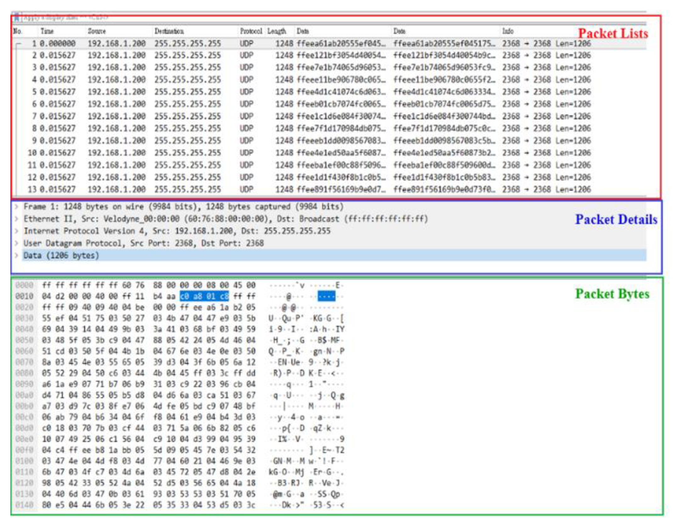
Figure 1 shows the package decoding. The red area will display all packets that include the number, time, packet protocol, and data quantity of the packet. The blue area further displays the selected packet details, including the number of bytes, packet protocol, device IP, and location information, etc. The green area displays the data content of the packet. This part is the original packet data required by our scheme. The required packet data are transferred to a standard format for subsequent decoding steps [1].
According to the angular resolution, different speeds will require different numbers of packets to restore to a map of horizontal angle (360°). Taking RPM600 as an example, the angular resolution is 0.1728°. Dividing a circle of 360 by 0.1728 and then dividing by 6 (a packet has only 6 horizontal angle movements), about 348 packets can be obtained, that is, 348 packets are needed to represent a 360° [1]. The rotation speed and the required number of packets are shown in Table 2.
The LiDAR packet structure has been introduced in the previous section. Each packet has a size of 1248 bytes, including header, data block, time stamp, status, and other information.
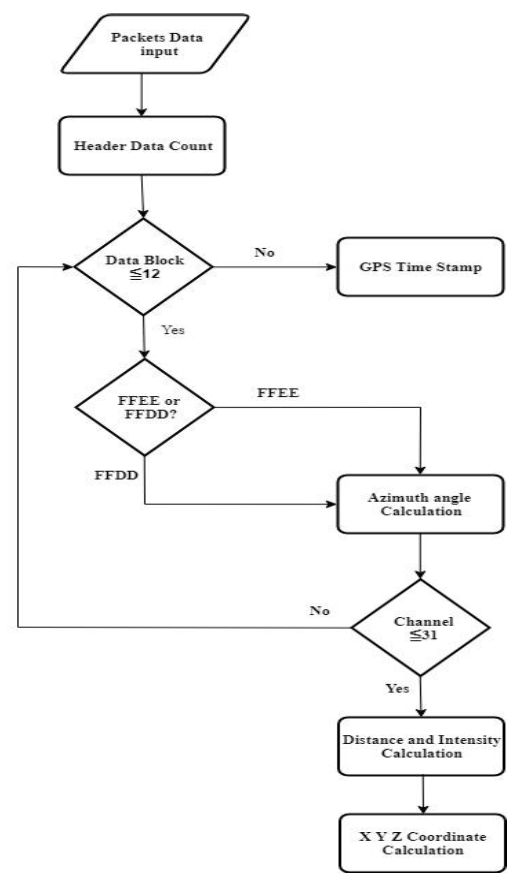
As shown in the LiDAR decoding flow chart in Figure 2, there will be 42 bytes of header file information in each header. Since the same information is provided in the header, the number of header files can be counted by a counter, and then 12 data blocks will be received. Each data block has a flag of 2 bytes. The hexadecimal FFEE represents the laser data in the upper area, FFDD represents the laser data in the lower area, and the laser data in the upper and lower areas. In pairs, Data Block 1 and 2 are a group, Data Block 3 and 4 are a group, and so on, so there are actually only 6 groups of complete data in a packet, and the next one will receive a 2 byte rotation position, that is, horizontal angle information. Each data block in the upper and lower areas of the packet will have the same horizontal angle information. Since the ranges of the horizontal angle are from 0° to 360°, when receiving the horizontal angle exceeds 360°, we can exchange the horizontal angle of 2 bytes and then convert it to decimal and divide by 100 to obtain the horizontal angle [1].
After obtaining the horizontal angle there will be 32 data points, divided into Channel 0 to Channel 31 to store the information, and each channel of information will provide 2 bytes of distance data and 1 byte of intensity data, and we can calculate distance through the distance data [1].
We convert the 2 bytes to decimal and multiply it by 2 to convert the unit to millimeter (mm), divide by 1000 and then convert the unit to meter (m), and the intensity data can be directly converted to decimal to analyze the reflectance. In addition, in each data block, a fixed vertical angle is provided in each channel, and each channel corresponds to an upper laser and a lower laser and has a fixed vertical angle. After receiving 12 data blocks, we will receive 4 bytes of GPS time stamp data. Finally, the packet will receive 2 bytes of status data [1].
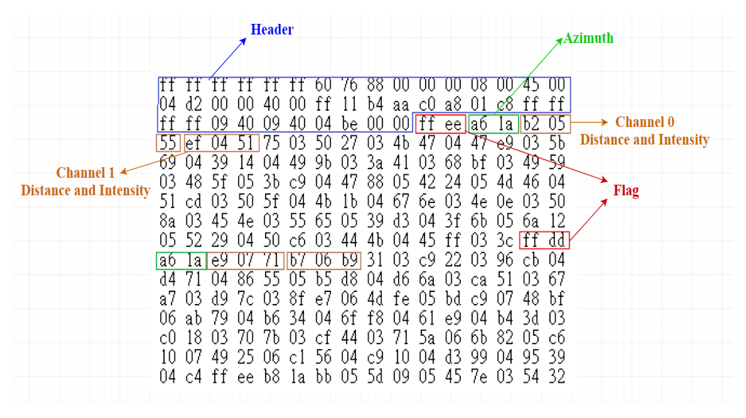
The actual packet diagram is shown in Figure 3, including the header of 42 bytes at the beginning, flag of 2 bytes, and Azimuth data of 2 bytes. The channel information is from 0 to 31. Each channel has 3 bytes of distance and 96 bytes of intensity data, respectively, which is a complete data block. It can be seen from the figure that the flags of Data Block 1 and Data Block 2 are FFEE and FFDD, respectively, but they have the same Azimuth data. Therefore, it can be determined that Data Block 1 and Data Block 2 represent the upper zone laser and the lower zone laser, respectively, which are obtained information at the same horizontal angle.
The paper takes the first group of data as an example, including Data Blocks 1 and 2, each representing the upper zone laser and the lower zone laser, and each has 32 channel data points. In Data Block 1, Channel 0 corresponds to the number 6. The upper zone laser has a vertical angle of −8.52. In Data Block 2, Channel 0 corresponds to the lower zone laser numbered 38. The vertical angle is −24.58. Therefore, the HDL-64 LiDAR used refers to the 64 channel. It means that two data blocks need to be occupied in the packet to represent 64 channel data.
After we complete the packet decoding, we can calculate the X, Y, and Z coordinates through the decoded horizontal angle, vertical angle, and distance, and use Equations (1)–(3) to calculate the X, Y, and Z coordinates as follows:
R represents the distance, that is, the distance data obtained by decoding, α represents the horizontal angle, and ω represents the vertical angle. After obtaining the X, Y, and Z coordinates, we reconstruct and display the point cloud image [1].
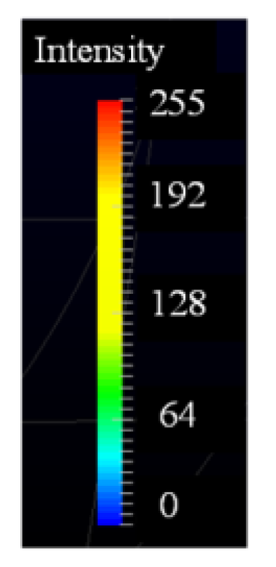
This paper uses the GL_POINTS function, which is commonly used to display geometric figure points, and the three-dimensional vector and function. The X, Y, and Z coordinates calculated in the previous section are brought into the three-dimensional vector and function, and the size and color of the point are defined through the GL_POINTS function. The color of the point is distinguished according to the intensity value, and it is divided into 10 levels from 0 to 255. The low-level value represents the lower value of intensity, which is represented by the blue color; the higher order value represents the higher value of intensity, which is shown in red.
The architecture of the “64-channel LiDAR packet decoding algorithm design” is implemented. It is mainly divided into packet capture, packet decoding, and point cloud image reconstruction. First, the necessary data in the original packet are captured, and the data are decoded into information such as distance, horizontal angle, and vertical angle. Finally, the information is converted into coordinates and reconstructed into a point cloud image.
4. Experimental Results
We will introduce the experimental methods and experimental results of this paper “64-channel LiDAR packet decoding algorithm design”. This section is divided into three parts. The first part introduces the experimental environment, including the instruments and environment settings we use, the second part introduces the experimental results and data analysis, and the third part lists the results compared with the literature. Finally, the fourth part is the conclusion.
The operating environment of the experiment is a notebook computer, and the operating system uses Microsoft (Redmond, WA, USA) Windows 10 (64 bit). The central processing unit (CPU) adopts Intel (Santa Clara, CA, USA) i7-8550U 1.8 GHz. The memory is 8 GB. The Graphic Processor uses Intel (Santa Clara, CA, USA) HD Graphics 620.
Among them, the paper adopts Velodyne HDL-64. The standard original packets used for the comparison of experimental data are all taken from the Map GMU (George Mason University) website [36]. In particular, the experimental team of GMU is setting up HDL- at 64, unlike the past, when the instrument was erected on the roof of the car, it was instead erected in the front of the car and perpendicular to the ground.
In the software operating environment, we use the pcap file format and use the Wireshark software to convert the packet format into a text file. For 3D image processing [37], we decode the packet into a coordinate system through C++ and restore it to a point cloud image.
We complete the experimental results and statistical analysis based on the research methods we proposed. The experiment takes a total of 10 scenes (10 pcap original files), each of which takes 3 pictures. According to the HDL-64 setting, the rotation rate is 10 revolutions per second. A complete 360° picture requires 348 frames such that it takes 348 packets, and finally records and compares the time of each image packet decoding and point cloud map imaging.
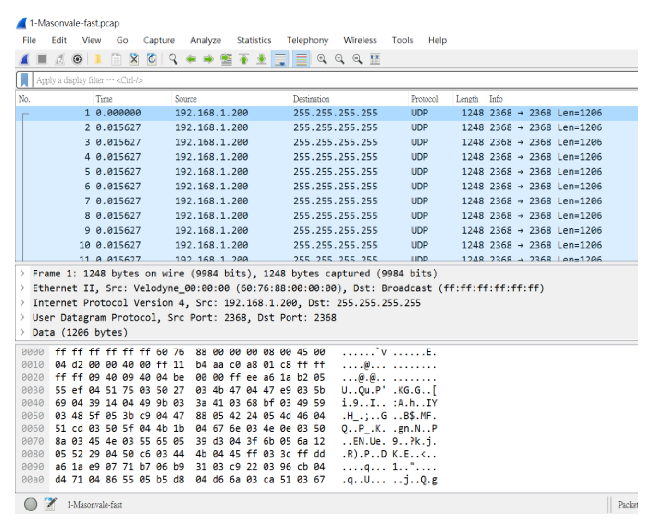
Then we introduce the extraction of each complete picture of each scene and the decoding process. First, take scenario 1 as an example, the original pcap file of Masonvale-fast-S16 downloaded from the Map GMU website, through Wireshark software, we know that this file has 302,487 frames (302,487 packets), as shown in Figure 4.
The top display shows the frame number, corresponding time, communication protocol, and packet size. The middle area shows the frame number, IP, port, and data size of the sending and receiving end, and the bottom displays the packet in hexadecimal notation and data content. In the first picture, we take the data content of frames 1 to 348 and convert it into a text file and decode it through our C++ program.
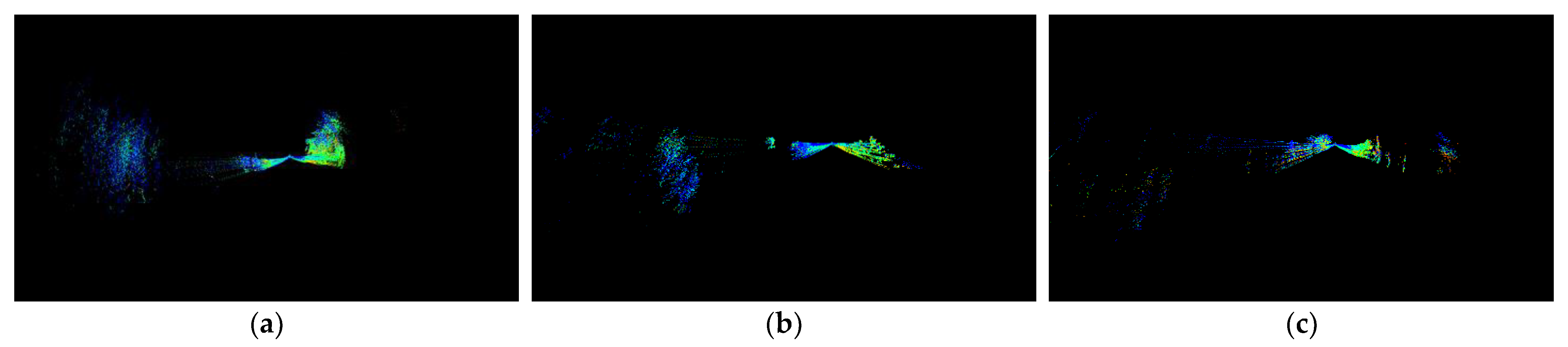
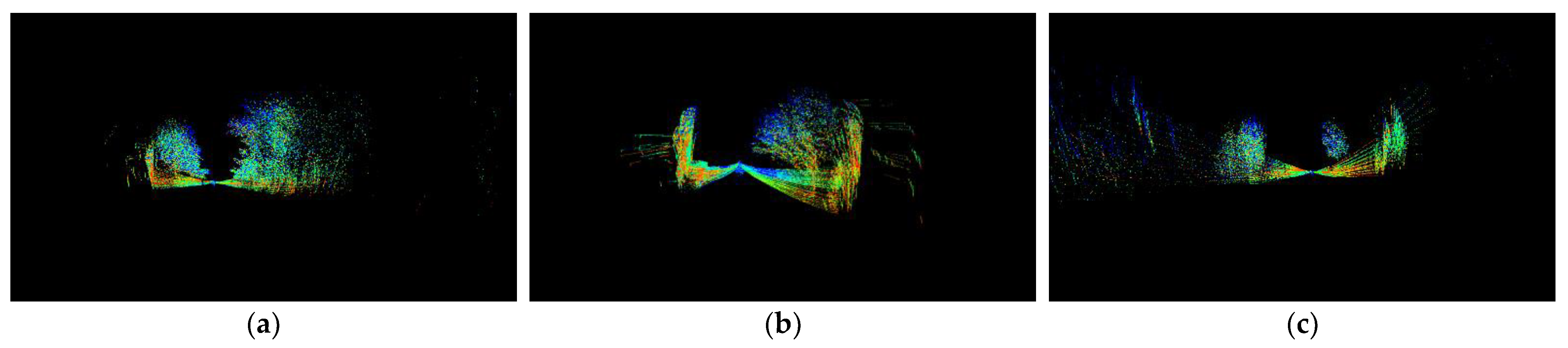
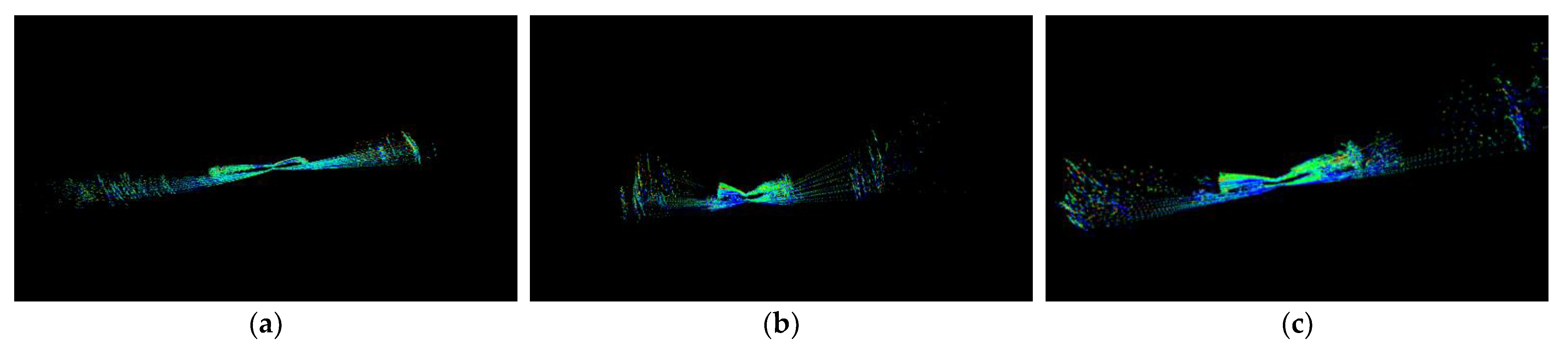
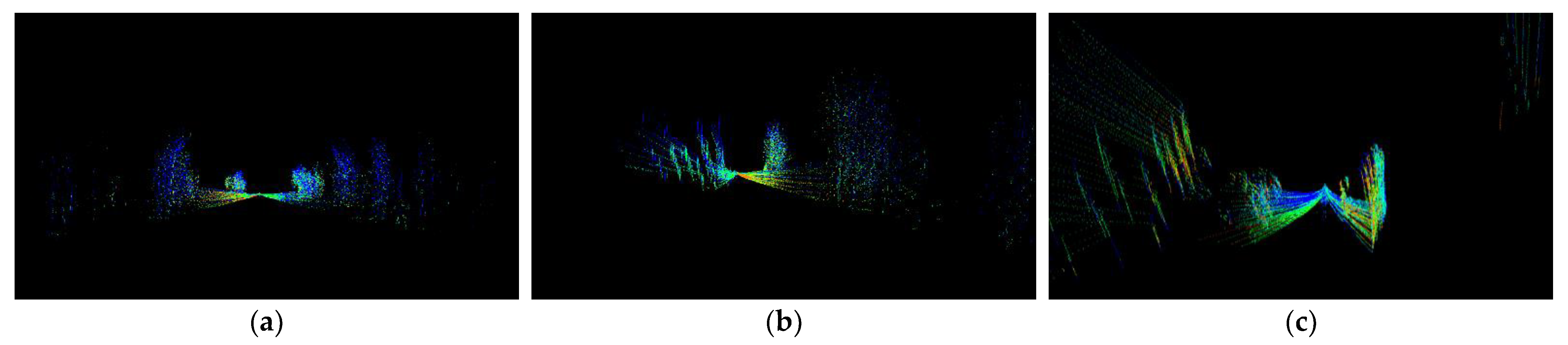
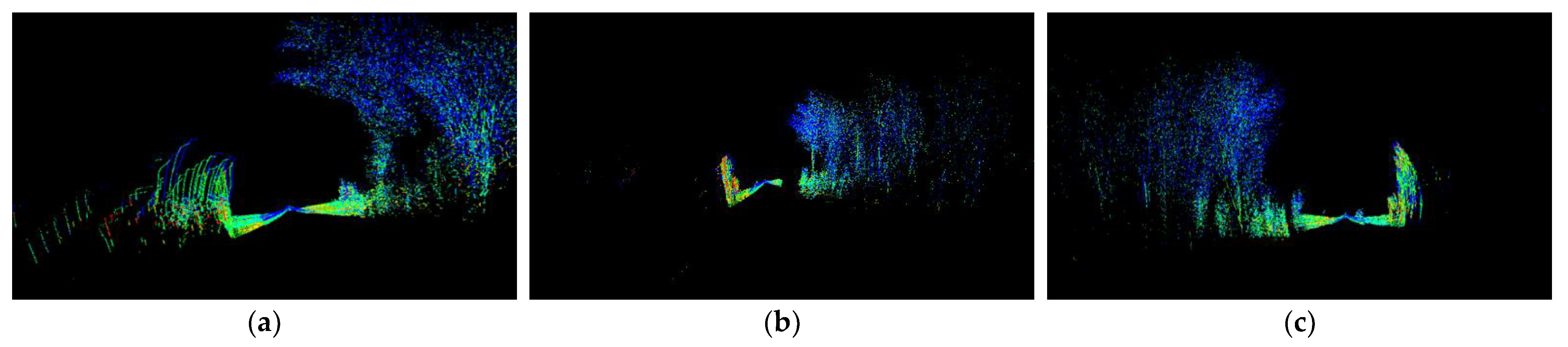
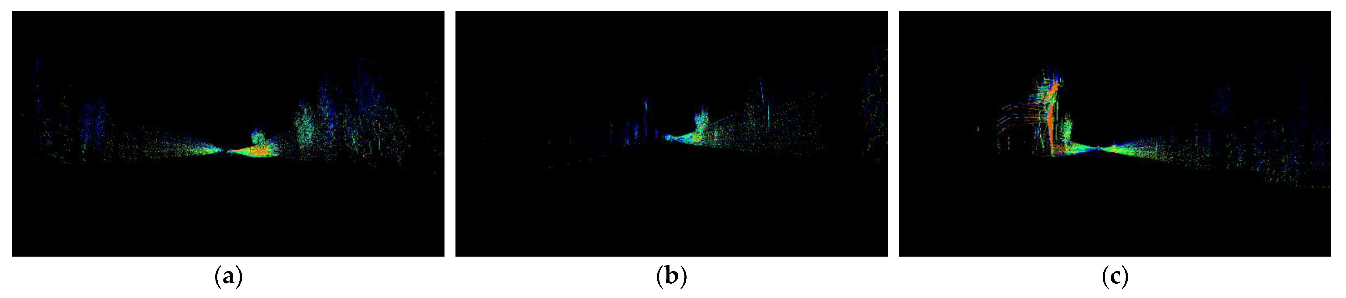
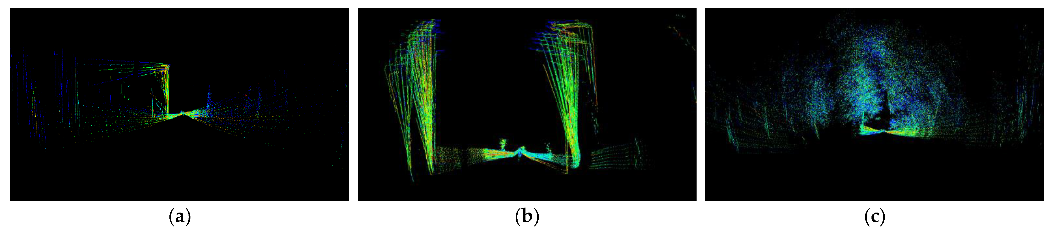
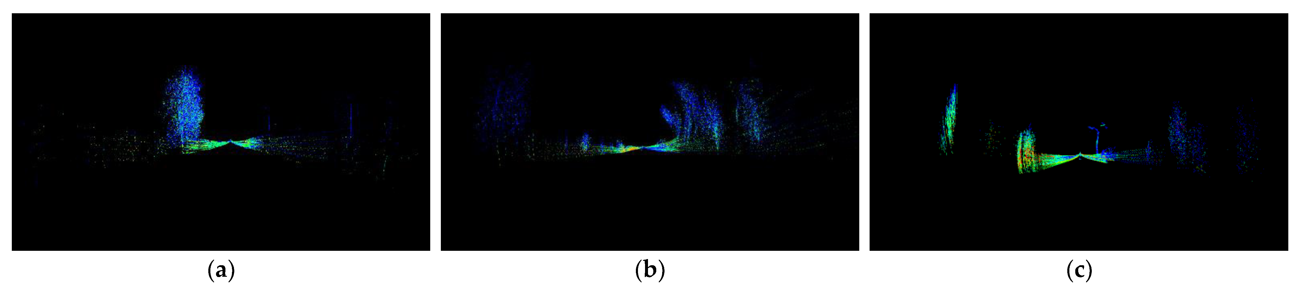
We will first compare the time required for the paper’s decoding process for different scenarios. In order to obtain the exact experimental value more accurately, each picture will be executed 3 times and the average value will be taken. The time information of 30 pictures is shown in Table 3. When each picture contains more packets, the gap will be more obvious. In addition, in order to highlight the difference between the experimental data, the 3 pictures in the same scene are specially selected for imaging 3 pictures with big differences [1]. The decoded point cloud image is shown in Figure 5, Figure 6, Figure 7, Figure 8, Figure 9, Figure 10, Figure 11, Figure 12, Figure 13 and Figure 14. There are 10 scenes in total, and each scene takes 3 pictures: (a) is Picture 1, (b) is Picture 2, and (c) is Picture 3. In addition, the imaging will also show the intensity, from 0 to 255, expressed in the three primary colors of RGB, as shown in Figure 15. The lower the intensity, the closer to blue, and the stronger the intensity, the closer to red.
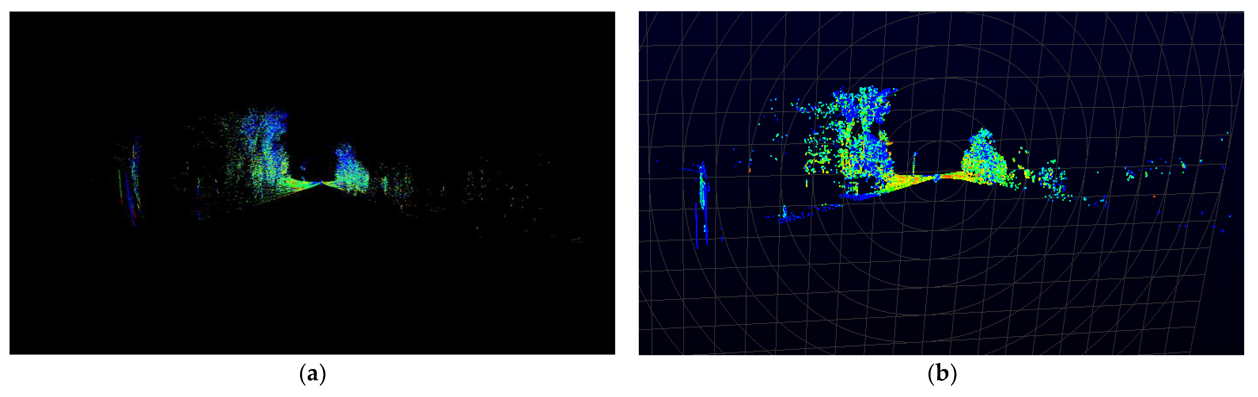
In addition, in order to verify whether the decoded three-dimensional LiDAR point clouds are correct, the ideal point cloud image with the reconstructed point cloud image are compared. After decoding, we can verify whether the decoding algorithm proposed is correct, as shown in Figure 16 (Figure 16a is the point cloud image reconstructed by the decoding algorithm proposed, Figure 16b is the ideal point cloud image). It can be seen from the figure that, although the color and a few details of the points are slightly different, this is because the difference caused by the different colors defined for different intensities, but the overall point cloud architecture can still be seen as the same picture, which proves that the three-dimensional coordinates derived by the decoding algorithm of this paper are correct [1].
Next, the experimental results of the decoding algorithm proposed are compared with the experimental results of the references, and the decoding processing time is discussed. Literature [38] mainly uses 16-channel VLP-16 LiDAR for static object detection, and the front part of the algorithm decodes the LiDAR packet to obtain the three-dimensional coordinates and reconstructs it into a point cloud image for horizontal and vertical clustering to obtain the edge of the object. The feature value is obtained by complementing the boundary of the object, which is used as a judgment to detect the object. The literature [39] proposed the point cloud image obtained through the light to make a feature judgment and, based on the result, to achieve the compensation of the plane depth information, thereby reconstructing a more complete point cloud image as the basis of object analysis. In addition, the image processing algorithm is used for plane detection, the vertex extraction of the plane is performed, the regular plane boundary is completed, and the plane information is finally supplemented to complete the reconstruction of the three-dimensional space. Since [38] and [39] both use VLP-16 as the experimental equipment, the number of packets contained in each picture is different from the HDL-64 used. The time is used as a basis for comparison, which is fairer and more objective. The comparison table is shown in Table 4. The average decoding time of a frame in [39] is 3.855 milliseconds. In [38], the average decoding time for a frame is 26.711 milliseconds. The average decoding time of a frame is 7.678 milliseconds. Although the time is about one times longer than that in [39], the data volume of HDL-64 is four times larger than that of HDL-16. Therefore, the calculation time of our algorithm must be divided by four times. Our algorithm is still faster than the literature [39]. Compared with the literature [38], the operation time of our algorithm saves three-quarters of the time. Combining the above test conditions, the decoding algorithm proposed has a better processing speed [1].
5. Discussion
From the aforementioned experiments, we can see that the greater the number of packets, the longer the decoding time, which increases proportionally, and it is much longer than the point cloud image reconstruction time. When the number of packets is larger, the gap becomes more obvious. Another key point of the experiment is to test whether the proposed algorithm correctly decodes and outputs three-dimensional coordinates. The point cloud image generated by the cross-comparison experiment and the point cloud image displayed by the official software provided by LiDAR can also prove this paper. The correctness of the decoding algorithm means that the algorithm proposed has a certain effect in the time spent on decoding and the correctness of the data [1]. The effectiveness of LiDAR can be seen from the experimental results. The car’s sensors that include radar, cameras, LiDAR, and GPS system were provided superhuman awareness of the surroundings [40,41]. The potential of the autonomous car to contribute to human flourishing is great [40,41]. If AI could drive autonomous cars, the human error that accounts for almost all of the 1.3 million deaths that happen on the world’s roads every year could be eradicated [40,41].
6. Conclusions
In this paper, we propose a decoding algorithm design based on 64-channel LiDAR packets. The proposed decoder mainly decodes the original LiDAR packet data and obtains XYZ coordinates. We reconstruct the image of the point cloud to verify that the decoded coordinates are correct. Recently, there is more and more LiDAR-related research. Many researchers focus on applications related to dynamic or static environment detection such as autonomous vehicles. LiDAR packet decoding is an important process before data calculation and recognition. This article proposes a 64-channel LiDAR packet decoding algorithm. The proposed decoder obtains three-dimensional coordinate data by capturing the content of the data packet and decoding the data packet and restores it to a point cloud image. The decoding algorithm we proposed has good performance in terms of data accuracy and packet decoding time.
Author Contributions
Y.-C.F. investigated the ideas, system, and methodology of the proposed techniques, and wrote the manuscript; S.-B.W. implemented the proposed system, conducted the experiments, analyzed the experimental data, and provided the analytical results. All authors discussed the results and contributed to the final manuscript. All authors have read and agreed to the published version of the manuscript.
Funding
This work was supported by the Ministry of Science and Technology of Taiwan under Grant MOST 109-2221-E-027-082.
Acknowledgments
The authors gratefully acknowledge the Taiwan Semiconductor Research Institute (TSRI) for supplying the technology models used in IC design.
Conflicts of Interest
The authors declare no conflict of interest.
References
- Wang, S.B.; Fan, Y.C. Three Dimensional Light Detection and Ranging Decoder Design. In Proceedings of the IEEE International Conference on Computer Communication and the Internet, Nagoya, Japan, 23–25 June 2021; pp. 10–14. [Google Scholar]
- Bastos, D.; Monteiro, P.P.; Oliveira, A.S.R.; Drummond, M.V. An Overview of LiDAR Requirements and Techniques for Autonomous Driving. In Proceedings of the Telecoms Conference (ConfTELE), Leiria, Portugal, 11–12 February 2021; pp. 1–6. [Google Scholar]
- Huang, R.; Chen, J.; Liu, J.; Liu, L.; Yu, B.; Wu, Y. A Practical Point Cloud Based Road Curb Detection Method for Autonomous Vehicle. Information 2017, 8, 93. [Google Scholar] [CrossRef] [Green Version]
- Liu, X.; Zhang, L.; Qin, S.; Tian, D.; Ouyang, S.; Chen, C. Optimized LOAM Using Ground Plane Constraints and SegMatch-Based Loop Detection. Sensors 2019, 19, 5419. [Google Scholar] [CrossRef] [PubMed]
- Wang, R.; Peethambaran, J.; Chen, C. LiDAR Point Clouds to 3-D Urban Models: A Review. IEEE J. Sel. Top. Appl. Earth Obs. Remote Sens. 2018, 11, 606–627. [Google Scholar] [CrossRef]
- Fernandez-Diaz, J.C.; Glennie, C.L.; Carter, W.E.; Shrestha, R.L.; Sartori, M.P.; Singhania, A.; Legleiter, C.J.; Overstreet, B.T. Early Results of Simultaneous Terrain and Shallow Water Bathymetry Mapping Using a Single-Wavelength Airborne LiDAR Sensor. IEEE J. Sel. Top. Appl. Earth Obs. Remote Sens. 2014, 7, 623–635. [Google Scholar] [CrossRef]
- Chen, Z.; Gao, B. An Object-Based Method for Urban Land Cover Classification Using Airborne Lidar Data. IEEE J. Sel. Top. Appl. Earth Obs. Remote Sens. 2014, 7, 4243–4254. [Google Scholar] [CrossRef]
- Yan, W.Y. Scan Line Void Filling of Airborne LiDAR Point Clouds for Hydroflattening DEM. IEEE J. Sel. Top. Appl. Earth Obs. Remote Sens. 2021, 14, 6426–6437. [Google Scholar] [CrossRef]
- Liang, X.; Wang, Y.; Jaakkola, A.; Kukko, A.; Kaartinen, H.; Hyyppä, J.; Honkavaara, E.; Liu, J. Forest Data Collection Using Terrestrial Image-Based Point Clouds from a Handheld Camera Compared to Terrestrial and Personal Laser Scanning. IEEE J. Sel. Top. Appl. Earth Obs. Remote Sens. 2015, 53, 5117–5132. [Google Scholar] [CrossRef]
- Höfle, B. Radiometric Correction of Terrestrial LiDAR Point Cloud Data for Individual Maize Plant Detection. IEEE Geosci. Remote Sens. Lett. 2014, 11, 94–98. [Google Scholar] [CrossRef]
- Fan, Y.-C.; Liu, Y.-C.; Chu, C.-A. Efficient CORDIC Iteration Design of LiDAR Sensors’ Point-Cloud Map Reconstruction Technology. Sensors 2019, 19, 5412. [Google Scholar] [CrossRef] [Green Version]
- Chen, J.-H.; Lin, G.-H.; Yelamandala, C.M.; Fan, Y.-C. High-Accuracy Mapping Design Based on Multi-view Images and 3D LiDAR Point Clouds. In Proceedings of the IEEE International Conference on Consumer Electronics, Las Vegas, NV, USA, 4–6 January 2020; pp. 1–2. [Google Scholar]
- Lee, S.-M.; Im, J.J.; Lee, B.-H.; Leonessa, A.; Kurdila, A. A Real-Time Grid Map Generation and Object Classification for Ground-Based 3D LIDAR Data using Image Analysis Techniques. In Proceedings of the IEEE International Conference on Image Processing, Hong Kong, China, 26–29 September 2010; pp. 2253–2256. [Google Scholar]
- Putman, E.B.; Popescu, S.C. Automated Estimation of Standing Dead Tree Volume Using Voxelized Terrestrial Lidar Data. IEEE Trans. Geosci. Remote Sens. 2018, 56, 6484–6503. [Google Scholar] [CrossRef]
- Engelcke, M.; Rao, D.; Wang, D.Z.; Tong, C.H.; Posner, I. Vote3Deep: Fast Object Detection in 3D Point Clouds Using Efficient Convolutional Neural Networks. In Proceedings of the IEEE International Conference on Robotics and Automation, Singapore, 29 May–3 June 2017; pp. 1355–1361. [Google Scholar]
- Zhang, Z.; Zhang, L.; Tong, X.; Mathiopoulos, P.T.; Guo, B.; Huang, X.; Wang, Z.; Wang, Y. A Multilevel Point-Cluster-Based Discriminative Feature for ALS Point Cloud Classification. IEEE Trans. Geosci. Remote Sens. 2016, 54, 3021–3309. [Google Scholar] [CrossRef]
- Rau, J.-Y.; Jhan, J.-P.; Hsu, Y.-C. Analysis of Oblique Aerial Images for Land Cover and Point Cloud Classification in an Urban Environment. IEEE Trans. Geosci. Remote Sens. 2015, 53, 1304–1319. [Google Scholar] [CrossRef]
- Wang, D.Z.; Posner, I.; Newman, P. What Could Move? Finding Cars, Pedestrians and Bicyclists in 3D Laser Data. In Proceedings of the IEEE International Conference on Robotics and Automation, Saint Paul, MN, USA, 14–18 May 2012; pp. 4038–4044. [Google Scholar]
- Xing, S.; Wang, D.; Xu, Q.; Lin, Y.; Li, P.; Jiao, L.; Zhang, X.; Liu, C. A Depth-Adaptive Waveform Decomposition Method for Airborne LiDAR Bathymetry. Sensors 2019, 19, 5065. [Google Scholar] [CrossRef] [Green Version]
- Ding, K.; Li, Q.; Zhu, J.; Wang, C.; Guan, M.; Chen, Z.; Yang, C.; Cui, Y.; Liao, J. An Improved Quadrilateral Fitting Algorithm for the Water Column Contribution in Airborne Bathymetric Lidar Waveforms. Sensors 2018, 18, 552. [Google Scholar] [CrossRef] [PubMed] [Green Version]
- Zhou, G.; Li, C.; Zhang, D.; Liu, D.; Zhou, X.; Zhan, J. Overview of Underwater Transmission Characteristics of Oceanic LiDAR. IEEE J. Sel. Top. Appl. Earth Obs. Remote Sens. 2021, 14, 8144–8159. [Google Scholar] [CrossRef]
- Matteoli, S.; Zotta, L.; Diani, M.; Corsini, G. POSEIDON: An Analytical End-to-End Performance Prediction Model for Submerged Object Detection and Recognition by Lidar Fluoros-ensors in the Marine Environment. IEEE J. Sel. Top. Appl. Earth Obs. Remote Sens. 2017, 10, 5110–5133. [Google Scholar] [CrossRef]
- Adams, M.D. Lidar Design, Use, and Calibration Concepts for Correct Environmental Detection. IEEE Trans. Robot. Autom. 2000, 16, 753–761. [Google Scholar] [CrossRef]
- Guan, H.; Yan, W.; Yu, Y.; Zhong, L.; Li, D. Robust Traffic-Sign Detection and Classification Using Mobile LiDAR Data with Digital Images. IEEE J. Sel. Top. Appl. Earth Obs. Remote Sens. 2018, 11, 1715–1724. [Google Scholar] [CrossRef]
- Okunsky, M.V.; Nesterova, N.V. Velodyne LIDAR method for sensor data decoding. In IOP Conference Series: Materials Science and Engineering; IOP Publishing: Bristol, UK, 2019; Volume 516, p. 012018. [Google Scholar]
- Zheng, L.-J.; Fan, Y.-C. Data Packet Decoder Design for LiDAR System. In Proceedings of the IEEE International Conference on Consumer Electronics-Taiwan, Taipei, Taiwan, 12–14 June 2017; pp. 35–36. [Google Scholar]
- Fan, Y.-C.; Mao, W.-L.; Tsao, H.-W. An Artificial Neural Network-Based Scheme for Fragile Watermarking. In Proceedings of the IEEE International Conference on Consumer Electronics, Los Angeles, CA, USA, 17–19 June 2003; pp. 210–211. [Google Scholar]
- Gergelova, M.B.; Labant, S.; Kuzevic, S.; Kuzevicova, Z.; Pavolova, H. Identification of Roof Surfaces from LiDAR Cloud Points by GIS Tools: A Case Study of Lučenec, Slovakia. Sustainability 2020, 12, 6847. [Google Scholar] [CrossRef]
- Shan, T.; Wang, J.; Chen, F.; Szenher, P.; Englot, B. Simulation-based Lidar Super-resolution for Ground Vehicles. Robot. Auton. Syst. 2020, 134, 103647. [Google Scholar] [CrossRef]
- Cugurullo, F.; Acheampong, R.A.; Gueriau, M.; Dusparic, I. The Transition to Autonomous Cars, the Redesign of Cities and the Future of Urban Sustainability. Urban Geogr. 2021, 42, 833–859. [Google Scholar] [CrossRef]
- Dowling, R.; McGuirk, P. Autonomous Vehicle Experiments and the City. Urban Geogr. 2020, 1–18. [Google Scholar] [CrossRef]
- Acheampong, R.A.; Cugurullo, F.; Gueriau, M.; Dusparic, I. Can Autonomous Vehicles Enable Sustainable Mobility in Future Cities? Insights and Policy Challenges from User Preferences Over Different Urban Transport Options. Cities 2021, 112, 103134. [Google Scholar] [CrossRef]
- Fan, Y.-C.; Chen, Y.-C.; Chou, S.-Y. Vivid-DIBR Based 2D–3D Image Conversion System for 3D Display. IEEE J. Disp. Technol. 2014, 10, 887–898. [Google Scholar]
- Fan, Y.-C.; Chiou, J.-C.; Jiang, Y.-H. Hole-Filling Based Memory Controller of Disparity Modification System for Multiview Three-Dimensional Video. IEEE Trans. Magn. 2011, 47, 679–682. [Google Scholar] [CrossRef]
- Velodyne Lidar. Available online: http://velodynelidar.com/downloads.html (accessed on 23 November 2021).
- Map GMU. Available online: http://masc.cs.gmu.edu/wiki/MapGMU (accessed on 23 November 2021).
- Fan, Y.-C.; You, J.-L.; Shen, J.-H.; Wang, C.-H. Luminance and Color Correction of Multiview Image Compression for 3-DTV System. IEEE Trans. Magn. 2014, 50, 1–4. [Google Scholar] [CrossRef]
- Ning, H.-I.; Fan, Y.-C. LiDAR Information for Objects Classified Technology in Static Environment. In Proceedings of the IEEE International Conference on Consumer Electronics-Taiwan, Taipei, Taiwan, 12–14 June 2017; pp. 127–128. [Google Scholar]
- Yang, S.-C.; Fan, Y.-C. 3D Building Scene Reconstruction Based on 3D LiDAR Point Cloud. In Proceedings of the IEEE International Conference on Consumer Electronics-Taiwan, Taipei, Taiwan, 12–14 June 2017; pp. 129–130. [Google Scholar]
- Stilgoe, J. Who’s Driving Innovation; New Technologies and the Collaborative State; Palgrave Macmillan: Cham, Switzerland, 2020. [Google Scholar]
- Cugurullo, F. Frankenstein Urbanism: Eco, Smart and Autonomous Cities, Artificial Intelligence and the End of the City; Routledge: New York, NY, USA, 2021. [Google Scholar]
Figure 1.
Package decoding.

Figure 2.
LiDAR decoding flow chart.

Figure 3.
The actual packet diagram.

Figure 4.
Wireshark software environment.

Figure 5.
Point cloud image scene 1: Masonvale-fast-S16 (a) Picture 1, (b) Picture 2, (c) Picture 3.
Figure 5.
Point cloud image scene 1: Masonvale-fast-S16 (a) Picture 1, (b) Picture 2, (c) Picture 3.

Figure 6.
Point cloud image scene 2: Nottoway-Annex-track5-fast-1loop (a) Picture 1, (b) Picture 2, (c) Picture 3.
Figure 6.
Point cloud image scene 2: Nottoway-Annex-track5-fast-1loop (a) Picture 1, (b) Picture 2, (c) Picture 3.

Figure 7.
Point cloud image scene 3: President-Park-Outside-S16 (a) Picture 1, (b) Picture 2, (c) Picture 3.
Figure 7.
Point cloud image scene 3: President-Park-Outside-S16 (a) Picture 1, (b) Picture 2, (c) Picture 3.

Figure 8.
Point cloud image scene 4: Shenandoah-4-fast (a) Picture 1, (b) Picture 2, (c) Picture 3.

Figure 9.
Point cloud image scene 5: Heating-S16 (a) Picture 1, (b) Picture 2, (c) Picture 3.

Figure 10.
Point cloud image scene 6: Masonvale (a) Picture 1, (b) Picture 2, (c) Picture 3.

Figure 11.
Point cloud image scene 7: Pond-counter-S16 (a) Picture 1, (b) Picture 2, (c) Picture 3.

Figure 12.
Point cloud image scene 8: Rappahanock (a) Picture 1, (b) Picture 2, (c) Picture 3.

Figure 13.
Point cloud image scene 9: Field-House-counter-S16 (a) Picture 1, (b) Picture 2, (c) Picture 3.
Figure 13.
Point cloud image scene 9: Field-House-counter-S16 (a) Picture 1, (b) Picture 2, (c) Picture 3.

Figure 14.
Point cloud image scene 10: Mason-Hall-S16 (a) Picture 1, (b) Picture 2, (c) Picture 3.

Figure 15.
Intensity of point cloud map.

Figure 16.
Point cloud comparison: (a) point cloud image of this paper, (b) ideal point cloud.


Table 1.
HDL-64 rotation rate and angular resolution comparison table [35].
Table 1.
HDL-64 rotation rate and angular resolution comparison table [35].
| RPM | RPS (Hz) | Total Laser Points per Revolution | Points per Laser per Revolution | Angular Resolution (Degrees) |
|---|---|---|---|---|
| 300 | 5 | 266,627 | 4167 | 0.0864 |
| 600 | 10 | 133,333 | 2083 | 0.1728 |
| 900 | 15 | 88,889 | 1389 | 0.2592 |
| 1200 | 20 | 66,657 | 1042 | 0.3456 |
Table 2.
HDL-64 rotation rate and the required number of packets.
| RPM | RPS (Hz) | Angular Resolution (Degrees) | Numbers of Packets Requirement |
|---|---|---|---|
| 300 | 5 | 0.0864 | ≒695 |
| 600 | 10 | 0.1728 | ≒348 |
| 900 | 15 | 0.2592 | ≒232 |
| 1200 | 20 | 0.3456 | ≒174 |
Table 3.
Time to reconstruct the point cloud image.
| Picture 1 | Picture 2 | Picture 3 | |
|---|---|---|---|
| Scene 1 | 0.083 | 0.106 | 0.094 |
| Scene 2 | 0.094 | 0.087 | 0.083 |
| Scene 3 | 0.102 | 0.159 | 0.159 |
| Scene 4 | 0.084 | 0.110 | 0.084 |
| Scene 5 | 0.083 | 0.085 | 0.148 |
| Scene 6 | 0.185 | 0.167 | 0.090 |
| Scene 7 | 0.095 | 0.176 | 0.085 |
| Scene 8 | 0.088 | 0.106 | 0.087 |
| Scene 9 | 0.085 | 0.084 | 0.083 |
| Scene 10 | 0.232 | 0.092 | 0.087 |
(Unit: second).
Publisher’s Note: MDPI stays neutral with regard to jurisdictional claims in published maps and institutional affiliations. |
© 2022 by the authors. Licensee MDPI, Basel, Switzerland. This article is an open access article distributed under the terms and conditions of the Creative Commons Attribution (CC BY) license (https://creativecommons.org/licenses/by/4.0/).
Share and Cite
MDPI and ACS Style
Fan, Y.-C.; Wang, S.-B. Three-Dimensional LiDAR Decoder Design for Autonomous Vehicles in Smart Cities. Information 2022, 13, 18. https://0-doi-org.brum.beds.ac.uk/10.3390/info13010018
AMA Style
Fan Y-C, Wang S-B. Three-Dimensional LiDAR Decoder Design for Autonomous Vehicles in Smart Cities. Information. 2022; 13(1):18. https://0-doi-org.brum.beds.ac.uk/10.3390/info13010018
Chicago/Turabian StyleFan, Yu-Cheng, and Sheng-Bi Wang. 2022. "Three-Dimensional LiDAR Decoder Design for Autonomous Vehicles in Smart Cities" Information 13, no. 1: 18. https://0-doi-org.brum.beds.ac.uk/10.3390/info13010018
Note that from the first issue of 2016, this journal uses article numbers instead of page numbers. See further details here.