
Logarithmic Negation of Basic Probability Assignment and Its Application in Target Recognition

College of Electronic Science and Technology, National University of Defense Technology, Changsha 410073, China
*
Author to whom correspondence should be addressed.
Information 2022, 13(8), 387; https://0-doi-org.brum.beds.ac.uk/10.3390/info13080387
Submission received: 12 July 2022
/
Revised: 10 August 2022
/
Accepted: 12 August 2022
/
Published: 15 August 2022
(This article belongs to the Special Issue New Trend on Fuzzy Systems and Intelligent Decision Making Theory: A Themed Issue Dedicated to Dr. Ronald R. Yager)
Abstract
:The negation of probability distribution is a new perspective from which to obtain information. Dempster–Shafer (D–S) evidence theory, as an extension of possibility theory, is widely used in decision-making-level fusion. However, how to reasonably construct the negation of basic probability assignment (BPA) in D–S evidence theory is an open issue. This paper proposes a new negation of BPA, logarithmic negation. It solves the shortcoming of Yin’s negation that maximal entropy cannot be obtained when there are only two focal elements in the BPA. At the same time, the logarithmic negation of BPA inherits the good properties of the negation of probability, such as order reversal, involution, convergence, degeneration, and maximal entropy. Logarithmic negation degenerates into Gao’s negation when the values of the elements all approach 0. In addition, the data fusion method based on logarithmic negation has a higher belief value of the correct target in target recognition application.
1. Introduction
Information fusion on the decision-making level is an important topic in artificial intelligence and machine learning. It can improve the performance of a system’s decision making very well. However, in the face of complex, uncertain, inaccurate, and incomplete information, how to efficiently fuse this information to obtain more reasonable results is a problem. For this problem, many theoretical tools were proposed, such as possibility theory [1,2,3], fuzzy set theory [4,5,6], Dempster–Shafer (D–S) evidence theory [7,8,9], D-numbers [10,11,12], Z-numbers [13,14,15], rough set theory [16,17,18], and fractal theory [19,20,21]. D–S evidence theory assigns probabilities to the power set of events, so it can effectively combine uncertain information. Therefore, it was widely applied to many real-world applications that include classification [22,23,24,25,26], fault diagnosis [27,28,29,30,31], decision making [32,33,34,35,36] and target recognition [37,38,39,40].
Events have two sides, so we often describe and express information from the front in D–S evidence theory. In fact, the opposite of an event can provide us with a new perspective and help us in obtaining more information in order to solve problems better. For example, if the highest probability of rain the next day is predicted to be 90%, it is still hard to make decisions, as the uncertainty cannot be determined. Let us see the negation of this situation. If the highest probability of not raining the next day is predicted to be 10%, decision making is relatively easy, and uncertainty is small [41]. On the basis of the above discussion, studying the negation of BPA [42,43,44,45] is of great significance to deal with uncertainty. How to reasonably construct the negation of BPA, on the other hand, is an open issue. Luo [41] proposed a matrix method of BPA negation where BPAs were represented as vectors, and negation was realized with matrix operators. This method could interpret the matrix operators well, but the calculation process was complicated. Gao [42] proposed a new negation that could be seen as arithmetic negation. It better presented the connection between changes in the uncertainty and entropy of random sets. Yin’s [44] negation of BPA could measure the uncertainty of the BPA well. However, the maximal entropy cannot be obtained when there are only two focal elements in the BPA. In this paper, we propose a novel negation of BPA based on the logarithmic function named logarithmic negation that can be seen as geometric negation and it solves the shortcoming of Yin’s negation. At the same time, the logarithmic negation of BPA inherits the good properties of negation of probability, such as order reversal, involution, convergence, degeneration, and maximal entropy. Logarithmic negation degenerates into Gao’s negation when the values of the elements all approach 0. In addition, the data fusion method based on logarithmic negation had a higher belief value of the correct target in the application of target recognition.
The remainder of this paper is organized as follows. The preliminaries are introduced in Section 2. In Section 3, the logarithmic negation is proposed, and its properties are analyzed and proved. In Section 4, some numerical examples are used to test the feasibility of logarithmic negation. In Section 5, two target recognition applications are used to demonstrate the effectiveness of the data fusion approach based on logarithmic negation. Conclusions are given in Section 6.
2. Preliminaries
2.1. D–S Evidence Theory
2.1.1. Frame of Discernment
was assumed to be a set of mutually exclusive and exhaustive elements and it could be defined as [46]:
where is the frame of discernment (FOD), and is the single subset proposition. We defined as a power set that contains elements and can be described as follows [47]:
where ⌀ is an empty set in Equation (2).
2.1.2. Basic Probability Assignment
Basic probability assignment (BPA) function m is also called mass function and is defined as a mapping of power set to [0,1] [48].
which satisfies
If , A is called a focal element or subset. Mass function is equal to 0 in classical D–S evidence theory.
2.2. Dempster’s Combination Rule
In D–S evidence theory, two BPAs can be combined with Dempster’s combination rule, defined as follows [49]:
in which
where ⊕ represents Dempster’s combination rule, and k is the conflict coefficient.
2.3. Shannon Entropy
Shannon entropy is an uncertain measure of information volume and is denoted by [50]:
where is the probability of state i.
2.4. Deng Entropy
Deng entropy is defined as follows [51]:
where is the cardinality of Proposition A.
2.5. Yin’s Negation of BPA
Yin’s negation of BPA is defined as follows [44]:
where n is the number of focal elements, and is the focal element.
2.6. Gao’s Negation of BPA
Gao’s negation of BPA is defined as follows [42]:
where n is the number of elements in the FOD, and is the mass function.
3. Proposed Negation
D–S evidence theory, with more accurate expression of information and better processing ability, is an extension of possibility theory. The negation of BPA shows the other side of the information and offers a new perspective on processing information. In this section, a new negation of BPA is proposed named logarithmic negation.
Assuming that the FOD has N elements, a power set is described as:
Since the negation of BPA is under classical D–S evidence theory, mass function was not considered. The power set can be expressed as:
which satisfies
The definition of logarithmic negation is as follows.
where N is the number of element in the FOD, and K is a normal number for every certain BPA. As we know,
then,
so
Then, we simplify and establish
Therefore,
is satisfied as the following conditions.
Theorem 1.
The logarithmic negation satisfies the order reversal. If , .
Proof.
If , we can obtain
Then,
□
Theorem 2.
The logarithmic negation satisfies the involution.
Proof.
□
Theorem 3.
As the number of iterations increases, logarithmic negation converges into .
Proof.
Assuming that represents the value of the tth iteration, represents the next moment after t. Since logarithmic negation is noninvolutionary, the value of negation constantly changes. if and only if , we can calculate the result of the next iteration as:
□
So, the negative value is fixed from the tth iteration, namely, converges into . Then, the belief distribution is uniform.
Theorem 4.
Logarithmic negation degenerates into Gao’s negation [42] when .
Proof.
According to the commonly used equivalent infinitesimal relations, we can obtain
When , we simplify and establish the following.
□
Theorem 5.
After each logarithmic negation operation, the entropy of information keeps increasing to its maximum.
Proof.
□
To further simplify the calculation, we could obtain the following approximation according to Theorem 4.
Then,
Through the Lagrangean multiplier method, we assume that
We then take the partial derivatives.
According to the derivation in [42], it can become
When the belief distribution of logarithmic negation follows uniform distribution, there is , and entropy reaches its maximum and cannot increase anymore.
Note: The more elements there are in the FOD, the faster the convergence speed is.
The more elements there are in FOD, the more uncertain information the BPA contains. Obviously, this has more elements involved in logarithmic negation. From the perspective of increasing entropy, the larger scale of FOD indicates that more elements consume information under the same conditions. Then, the overall rate of the consumption of information is faster, entropy reaches its maximum more quickly, and the belief distribution quickly converges. Furthermore, the larger the number of elements is, the smaller the logarithmic negation that converges into the value of . Thus, belief redistribution by logarithmic negation facilitates the belief distribution to converge into uniform distribution. This is illustrated by numerical Examples 2–4.
The phenomenon of logarithmic negation measures the uncertainty of evidence by reassigning belief. From the point of view of information entropy, the essence of logarithmic negation is the process of consuming information, and the entropy converges into maximal entropy. Detailed numerical examples in the next section are given to help in understanding the concept.
4. Numerical Examples
In the next section, several numerical examples are used to illustrate the theorems.
Example 1.
The FOD is assumed to be in the close world. The BPA is .
Yin’s negation of BPA is
Yin’s negation [44] method cannot handle this special case where there is one focal element in the close world. Since Yin’s negation can only construct negations from elements with belief values greater than 0, this inevitably causes a loss of information in the FOD and produces unreasonable results.
The logarithmic negation of BPA is
Obviously, the proposed negation could obtain the intuitive results. Although BPAs were equal to 0, they contained important information, that is, events b and were unlikely to happen. The proposed method could capture this hidden information and process it to render the expression of information more complete and effective.
Example 2.
The FOD was assumed to be in the close world. The BPA is .
Yin’s negation of BPA is
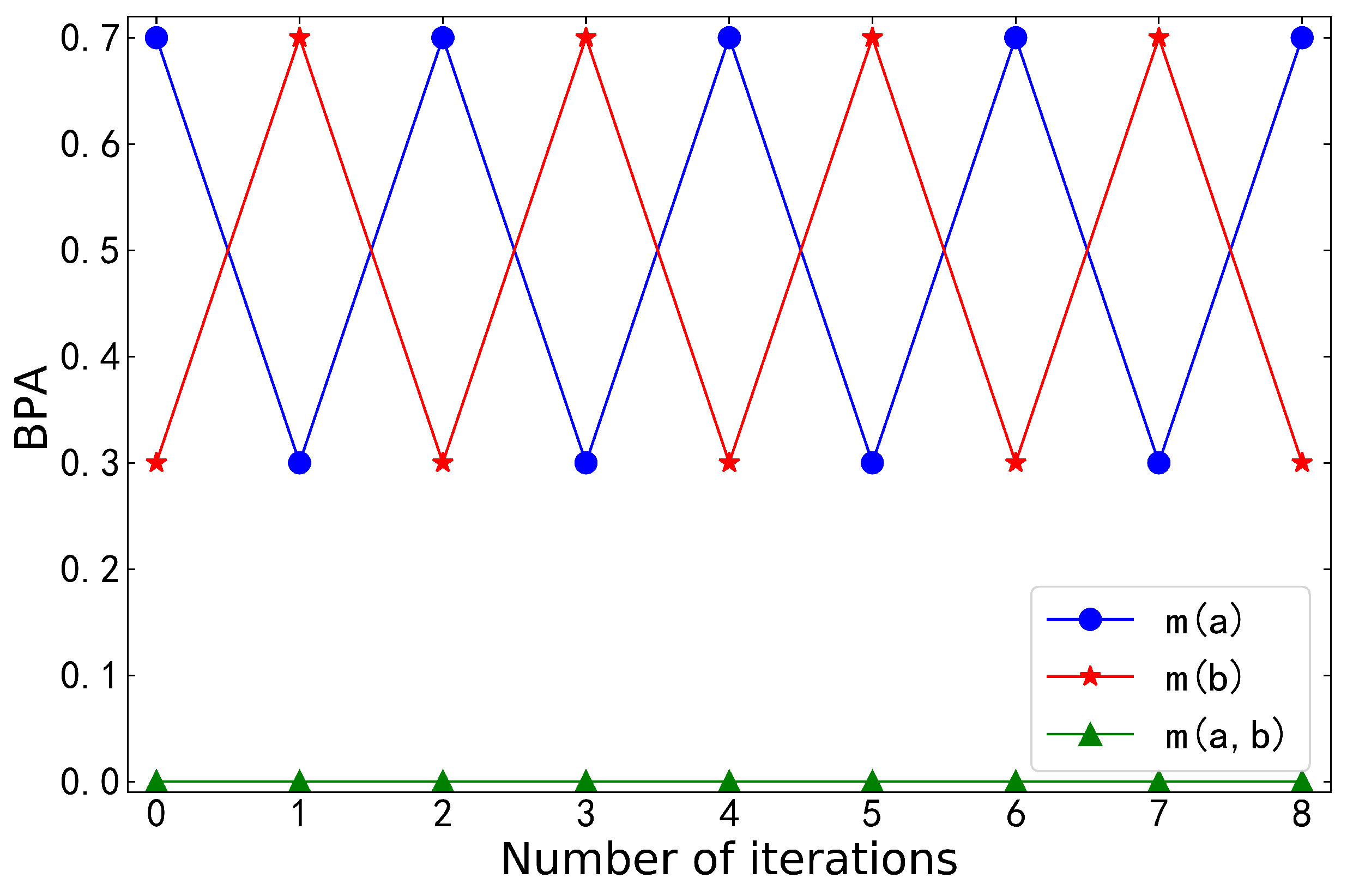
Table 1 shows the BPA and entropy after Yin’s negation iterations, and Figure 1 visualizes them. When the BPA only contained two focal elements, the negation was reversible: . No matter the number of negation iterations, the belief values of and always cyclically changed between 0.7 and 0.3. This did not converge into a certain value. Correspondingly, entropy no longer increased and could not reach its maximum.
The logarithmic negation of BPA is
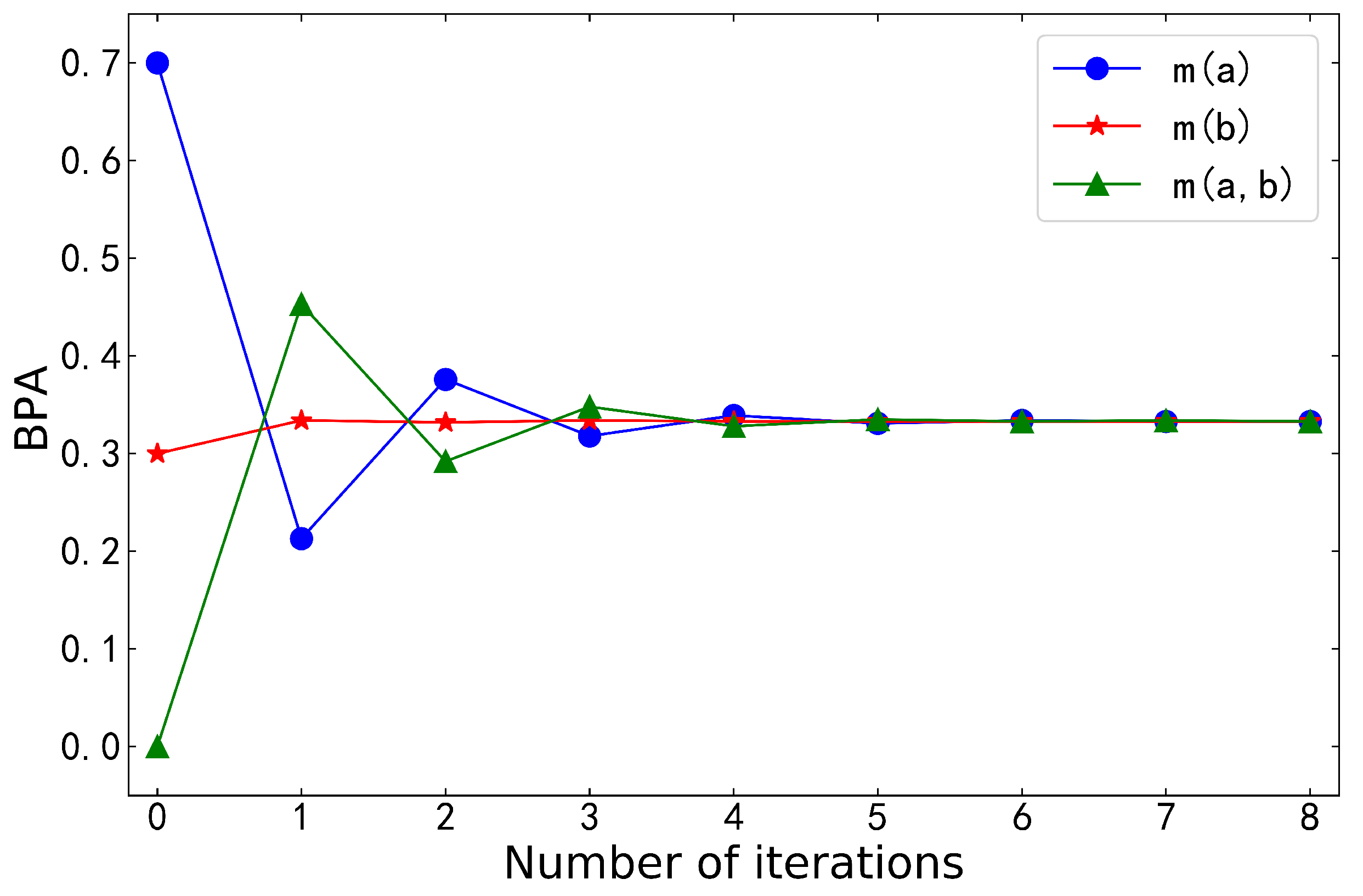
The above shows that when , which is consistent with the order reversal. In addition, there is . The irreversibility was verified. Table 2 shows the BPA and entropy after logarithmic negation iteration, and Figure 2 visualizes them. The belief distribution lastly converged into uniform distribution, that is, the negative values were all equal to . Entropy kept increasing to its maximum. Theorems 3 and 5 were fully verified. The proposed negation overcomes the shortcomings of Yin’s negation well.
Example 3.
The FOD was assumed to be in the close world. The BPA is .
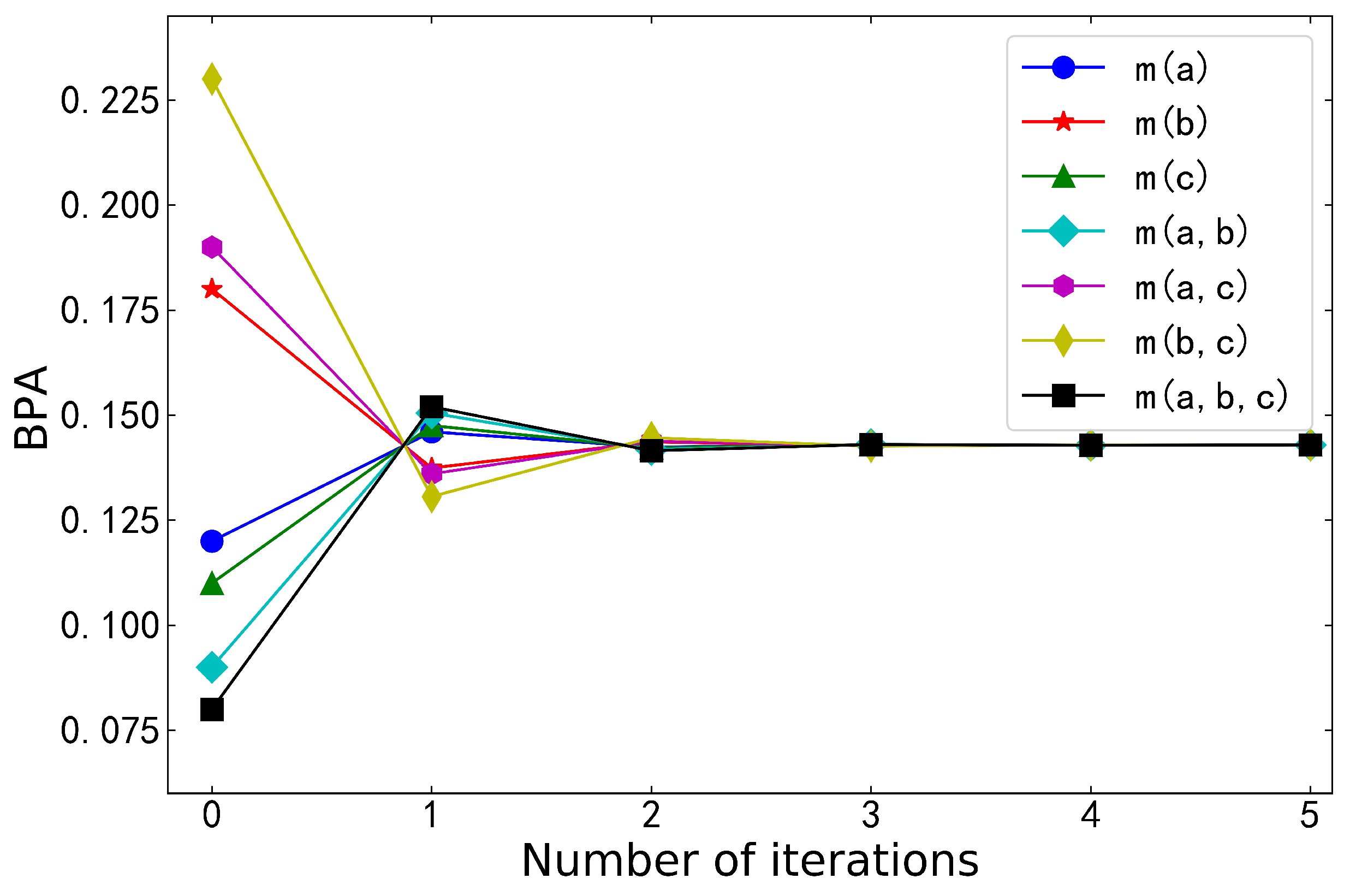
Table 3 shows the BPA and entropy after logarithmic negation iterations, and Figure 3 visualizes them. The belief distribution gradually converged as the number of iterations increased. Lastly, the BPA converged into uniform distribution. At the same time, maximal entropy was obtained. We can understand this phenomenon in terms of information consumption. In fact, each iteration of negation is a process of consuming information. The consumption of information means an increase in entropy. When maximal entropy was reached, there was no more information to consume for the BPA, and entropy stopped increasing. Theorems 3 and 5 of logarithmic negation were verified again.
Example 4.
The FOD was assumed to be in the close world. The BPA is .
Table 4 shows the BPA and entropy after logarithmic negation iterations. The FOD contained two elements in Example 2, three elements in Example 3, and four elements in Example 4. Table 2, Table 3 and Table 4 show that the numbers of iterations required for the convergence of a logarithmic negative were 8, 5, and 4. In other words, the convergence speed of logarithmic negation accelerated significantly as the scale of the FOD grew. This means that the BPA needed fewer negative iterations to obtain maximal entropy. This interesting point is understood from the perspective of increasing entropy. The larger scale of FOD indicates that more elements consumed information under the same conditions. Then, the overall rate of consumption of information was faster. Thus, maximal entropy was achieved faster.
5. Application
In this section, two target recognition applications are used to verify the effectiveness of the data fusion approach based on the logarithmic negation. On the basis of the proposed negation, we adopted Li’s data fusion method [45] to run the target recognition application. The detailed steps of Li’s method are described as follows.
Step 1: construct the logarithmic negation of each piece of evidence by using Equation (12), where n is the number of pieces of evidence.
Step 2: calculate the Deng entropy of the initial evidence and its negation by using Equation (6).
Step 3: calculate the credibility of each piece of evidence by using Equation (16).
where represents the absolute value of the entropy difference between the initial evidence and its negation. If the belief distribution is uniform, we just need to replace with .
Step 4: calculate the weight of each piece of evidence by using Equation (17).
Step 5: weighted average evidence is calculated as follows:
Step 6: Dempster’s combination rule is used k-1 times to combine the weighted average evidence according to Equation (3). Then, the final combination result is calculated as follows:
5.1. Application 1
In a multisensor automatic target recognition system, it is assumed that the actual target is A. The collected sensor reports from the system, modelled as BPAs, are shown in Table 5. The application is cited from [45].
Step 5: weighted average evidence is calculated as follows:
Step 6: Dempster’s combination rule is used 3 times to combine the weighted average evidence according to Equation (3). Then, the final combination result is calculated as follows:
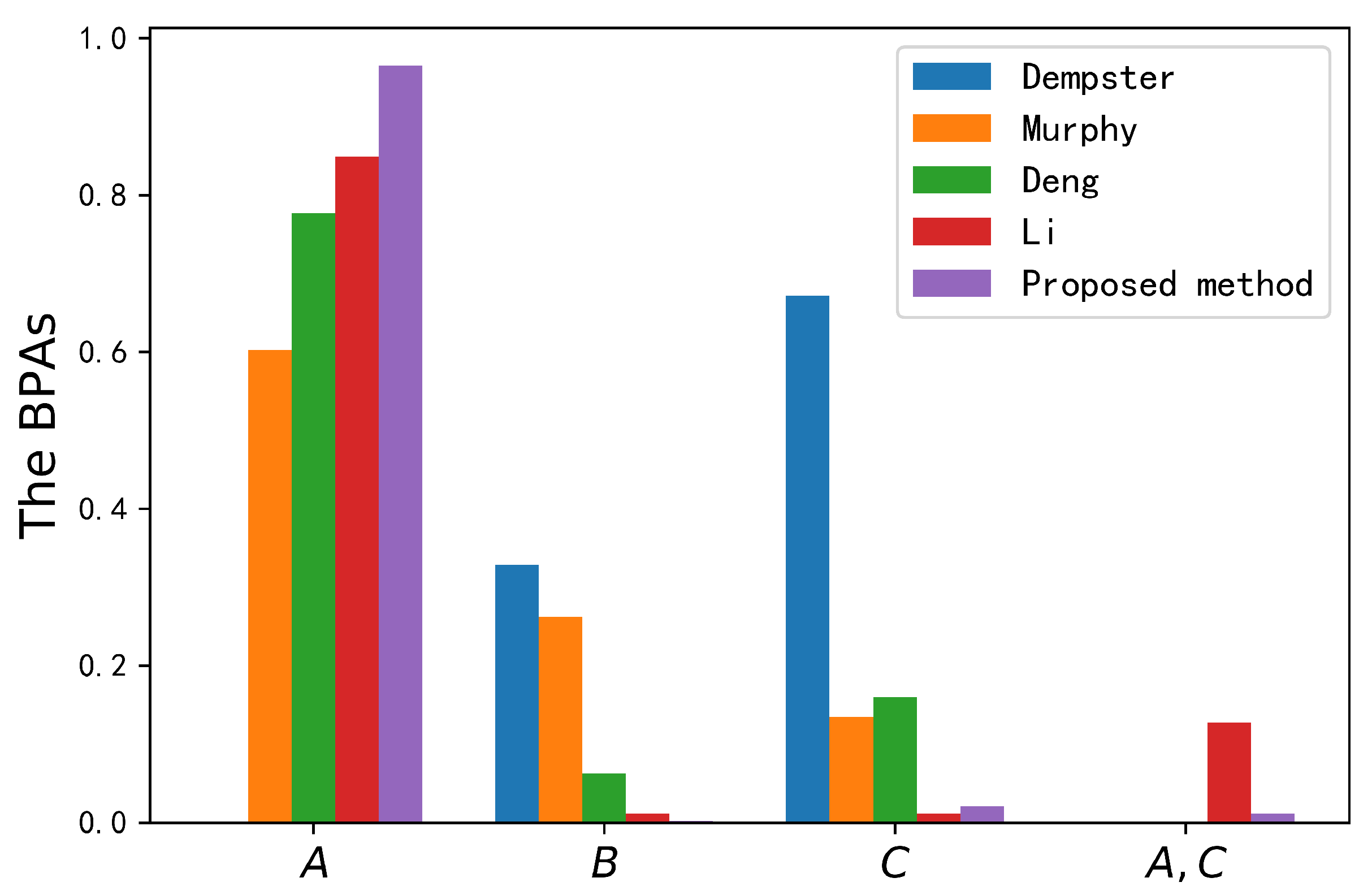
Evidence is highly conflicted with other pieces of evidence. As shown in Table 6 and Figure 4, Dempster’s method did not identify the correct target A. The operation of a one-vote vet produced a counterintuitive result that the belief value of target A is always 0. However, other methods all overcame the impact of conflicting evidence and obtained reasonable decision-making results. The experimental results show that the belief value of the correct target A for the three other methods was 0.6027, 0.7773 and 0.8491. The degree of belief was relatively low. The proposed data fusion method could achieve better performance in combining pieces of conflicting evidence, as it had the highest belief value (0.9653) for the correct target A. Compared with the three other methods, the belief value of the correct target was improved by 36.26%, 17.8% and 11.62%. The main reason is that the logarithmic negation could extract more useful information in the process of conflict processing from the perspective of geometric negation. The accuracy of the fusion results was improved, and the target type could be identified more accurately. Furthermore, since the entropy of conflicting evidence is usually low, it can distinguish between conflicting and normal evidence with Deng entropy. The entropy difference between the conflicting evidence and its negation was larger than that of normal evidence. Therefore, the proposed method assigned a lower credibility value to the conflicting evidence, and more reasonable results were obtained. This application proves the validity of the proposed method.
5.2. Application 2
Consider a multisensor target recognition problem associated with sensor reports that are collected from five different types of sensors , and each of which is allocated to a different position in order to monitor the objectives. The FOD that consists of three types of target is given by . These sensors collect the target information and generate reports, which were modeled as BPAs denoted by and in Table 7. The application is cited from [54].
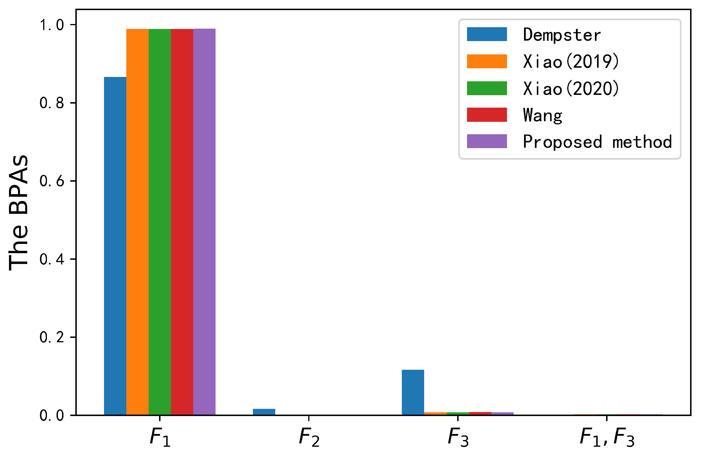
The combined results are shown in Figure 5 and Table 8. Even if the second piece of evidence was in major conflict with other evidence, all the methods could successfully identify the target type as A, which was in line with our intuition. The belief value of the target type A for the four other methods is 0.8657, 0.9885, 0.9888 and 0.9892. Although the overall belief value was relatively high, the accuracy of the fusion results still has some room for improvement. The proposed method had the highest belief value (0.9897) for the correct target. The belief value of the correct target with the proposed method was only improved by 0.05% compared with Wang’s method [55], but it is of great significance to the target recognition system based on such a high belief value. The main reason is that the proposed method took more uncertainty information into account in the process of logarithmic negation of BPA, that is, it used well the information of elements whose belief value was equal to 0. The operation of logarithmic negation consumed a lot of information in the conflicting evidence, which led to a rapid increase in the entropy of the conflicting evidence’s negation. Then, the entropy difference between the conflicting evidence and its negation grew, and the conflicting evidence was assigned a smaller weight value. Lastly, conflicting evidence was handled effectively. In addition, the combination of Deng entropy and logarithmic negation improved the accuracy of the fusion results and reduced the loss of information, which also ensured the ability to deal with conflicting evidence. The validity of the proposed method was verified again.
6. Conclusions
How to reasonably construct the negation of BPA is an open issue. To address this problem, a novel negation of BPA was proposed named logarithmic negation that solves the shortcoming of Yin’s negation that the maximal entropy cannot be obtained when there are only two focal elements in the BPA. At the same time, the logarithmic negation of BPA inherits the good properties of the negation of probability, such as order reversal, involution, convergence, degeneration, and maximal entropy. Logarithmic negation degenerates into Gao’s negation when the values of the elements all approach 0. The operation of logarithmic negation can cause an increase in entropy, and convergence speed is proportional to the number of elements in the FOD. Some numerical examples were presented for analysis and proof. Lastly, the data fusion method based on logarithmic negation had the highest belief value of the correct target in two target recognition applications.
Author Contributions
Conceptualization, S.X., Y.H. and X.D.; Data curation, Y.H.; Formal analysis, Y.H., P.C. and S.Z.; Funding acquisition, Y.H., P.C. and S.Z.; Investigation, Y.H., P.C. and S.Z.; Methodology, S.X., Y.H. and X.D.; Project administration, S.X., Y.H. and X.D.; Resources, S.X., Y.H. and X.D.; Software, Y.H., P.C. and S.Z.; Supervision, Y.H., P.C. and S.Z.; Validation, S.X. and Y.H.; Writing—original draft, S.X. and Y.H.; Writing—review & editing, S.X. and Y.H. All authors have read and agreed to the published version of the manuscript.
Funding
This research was supported by the National Natural Science Foundation of China (Grant No.61903373 and 61921001).
Institutional Review Board Statement
Not applicable.
Informed Consent Statement
Not applicable.
Data Availability Statement
Not applicable.
Conflicts of Interest
The authors declare no conflict of interest.
References
- Hose, D.; Hanss, M. A universal approach to imprecise probabilities in possibility theory. Int. J. Approx. Reason 2021, 133, 133–158. [Google Scholar] [CrossRef]
- Yin, H.; Huang, J.; Chen, H. Possibility-based robust control for fuzzy mechanical systems. IEEE Trans. Fuzzy Syst. 2020, 99, 1. [Google Scholar] [CrossRef]
- Gu, Q.; Xuan, Z. A new approach for ranking fuzzy numbers based on possibility theory. J. Comput. Appl. Math. 2017, 309, 674–682. [Google Scholar] [CrossRef]
- Meng, L.; Li, L. Time-sequential hesitant fuzzy set and its application to multi-attribute decision making. J. Complex Intell. Syst. 2022, 1–20. [Google Scholar] [CrossRef]
- Moko, J.; Hurtík, P. Approximations of fuzzy soft sets by fuzzy soft relations with image processing application. Soft Comput. 2021, 25, 6915–6925. [Google Scholar] [CrossRef]
- Hja, B.; Bao, Q. A decision-theoretic fuzzy rough set in hesitant fuzzy information systems and its application in multi-attribute decision-making. Inform. Sci. 2021, 579, 103–127. [Google Scholar] [CrossRef]
- Chen, Z.; Cai, R. A novel divergence measure of mass function for conflict management. Int. J. Intell. Syst. 2022, 37, 3709–3735. [Google Scholar] [CrossRef]
- Liu, J.; Tang, Y. Conflict data fusion in a multi-agent system premised on the base basic probability assignment and evidence distance. Entropy 2021, 23, 820. [Google Scholar] [CrossRef]
- Tong, Z.; Xu, P.; Denaux, T. An evidential classifier based on Dempster–Shafer theory and deep learning. Neurocomputing 2021, 450, 275–293. [Google Scholar] [CrossRef]
- Mi, X.; Tian, Y.; Kang, B. A hybrid multi-criteria decision making approach for assessing health-care waste management technologies based on soft likelihood function and d-numbers. Appl. Intell. 2021, 2, 1–20. [Google Scholar] [CrossRef]
- Lai, H.; Liao, H. A multi-criteria decision making method based on DNMA and CRITIC with linguistic D numbers for blockchain platform evaluation. Eng. Appl. Artif. Intell. 2021, 101, 104200. [Google Scholar] [CrossRef]
- Liu, P.; Zhu, B.; Wang, P. A weighting model based on best–worst method and its application for environmental performance. Appl. Soft Comput. 2021, 103, 107168. [Google Scholar] [CrossRef]
- Jia, Q.; Hu, J. A novel method to research linguistic uncertain Z-numbers. Inform. Sci. 2022, 586, 41–58. [Google Scholar] [CrossRef]
- Hu, Z.; Lin, J. An integrated multicriteria group decision making methodology for property concealment risk assessment under Z-number environment. Expert Syst. Appl. 2022, 205, 117369. [Google Scholar] [CrossRef]
- Yousefi, S.; Valipour, M.; Gul, M. Systems failure analysis using Z-number theory-based combined compromise solution and full consistency method. Appl. Soft Comput. 2021, 113, 107902. [Google Scholar] [CrossRef]
- Yu, Z.; Wang, D.; Wang, P. A study of interrelationships between rough set model accuracy and granule cover refinement processes. Inform. Sci. 2021, 578, 116–128. [Google Scholar] [CrossRef]
- Jin, C.; Mi, J.; Li, F. A novel probabilistic hesitant fuzzy rough set based multi-criteria decision-making method. Inform. Sci. 2022, 608, 489–516. [Google Scholar] [CrossRef]
- Zhang, X.; Jiang, J. Measurement, modeling, reduction of decision-theoretic multigranulation fuzzy rough sets based on three-way decisions. Inform. Sci. 2022, 607, 1550–1582. [Google Scholar] [CrossRef]
- Wang, H.; Liu, S.; Qu, X. Field investigations on rock fragmentation under deep water through fractal theory. Measurement 2022, 199, 111521. [Google Scholar] [CrossRef]
- Zhou, Z.; Zhao, C.; Cai, X. Three-dimensional modeling and analysis of fractal characteristics of rupture source combined acoustic emission and fractal theory. Chaos Solitons Fractals 2022, 160, 112308. [Google Scholar] [CrossRef]
- Liu, W.; Yan, S.; Chen, T. Feature recognition of irregular pellet images by regularized Extreme Learning Machine in combination with fractal theory. Future Gener. Comp. Syst. 2022, 127, 92–108. [Google Scholar] [CrossRef]
- Wu, D.; Liu, Z.; Tang, Y. A new classification method based on the negation of a basic probability assignment in the evidence theory. Eng. Appl. Artif. Intell. 2020, 127, 92–108. [Google Scholar] [CrossRef]
- Zhao, K.; Li, L.; Chen, Z. A New Multi-classifier Ensemble Algorithm Based on D–S Evidence Theory. Neural Process. Lett. 2022. [Google Scholar] [CrossRef]
- Zhang, X.; Yang, Y.; Li, T. CMC: A Consensus Multi-view Clustering Model for Predicting Alzheimer’s Disease Progression. Comput. Meth. Prog. Biomed. 2021, 199, 105895. [Google Scholar] [CrossRef]
- Yang, F.; Wei, H.; Feng, P. A hierarchical Dempster–Shafer evidence combination framework for urban area land cover classification. Measurement 2020, 151, 105916. [Google Scholar] [CrossRef]
- Peñafiel, S.; Baloian, N.; Sanson, H. Applying Dempster–Shafer theory for developing a flexible, accurate and interpretable classifier. Expert Syst. Appl. 2020, 148, 113262. [Google Scholar] [CrossRef]
- Ji, X.; Ren, Y.; Tang, H. An intelligent fault diagnosis approach based on Dempster–Shafer theory for hydraulic valves. Measurement 2020, 165, 108129. [Google Scholar] [CrossRef]
- Verbert, K.; Babuška, R.; Schutter, B. Bayesian and Dempster–Shafer reasoning for knowledge-based fault diagnosis—A comparative study. Eng. Appl. Artif. Intell. 2017, 60, 136–150. [Google Scholar] [CrossRef]
- Gao, X.; Xiao, F. A generalized χ2 divergence for multisource information fusion and its application in fault diagnosis. Int. J. Intell. Syst. 2022, 37, 5–29. [Google Scholar] [CrossRef]
- Tingfang, Y.; Haifeng, L.; Xiangjun, Z.; Wei, Q.; Wenbin, D. Application of a combined decision model based on optimal weights in incipient faults diagnosis for power transformer. IEEE Trans. Elect. Electron. Eng. 2016, 12, 169–175. [Google Scholar] [CrossRef]
- Xu, Y.; Li, Y.; Wang, Y.; Wang, C.; Zhang, G. Integrated decision-making method for power transformer fault diagnosis via rough set and DS evidence theories. IET Gener. Transm. Distrib. 2020, 14, 5774–5781. [Google Scholar] [CrossRef]
- Dymova, L.; Sevastjanov, P. An interpretation of intuitionistic fuzzy sets in terms of evidence theory: Decision making aspect. Knowl.-Based Syst. 2010, 23, 772–782. [Google Scholar] [CrossRef]
- Li, Z.; Wen, G.; Xie, N. An approach to fuzzy soft sets in decision making based on grey relational analysis and Dempster–Shafer theory of evidence: An application in medical diagnosis. Artif. Intell. Med. 2015, 64, 161–171. [Google Scholar] [CrossRef] [PubMed]
- Liu, P.; Gao, H. Some intuitionistic fuzzy power Bonferroni mean operators in the framework of Dempster–Shafer theory and their application to multicriteria decision making. Appl. Soft Comput. 2019, 85, 105790. [Google Scholar] [CrossRef]
- Xiao, F. EFMCDM: Evidential Fuzzy Multicriteria Decision Making Based on Belief Entropy. IEEE Trans. Fuzzy Syst. 2020, 28, 1477–1491. [Google Scholar] [CrossRef]
- Xiao, F.; Cao, Z.; Jolfaei, A. A Novel Conflict Measurement in Decision-Making and Its Application in Fault Diagnosis. IEEE Trans. Fuzzy Syst. 2021, 29, 186–197. [Google Scholar] [CrossRef]
- Liu, M.; Wu, Y.; Zhao, W.; Zhang, Q.; Liao, G. Dempster–Shafer Fusion of Multiple Sparse Representation and Statistical Property for SAR Target Configuration Recognition. IEEE Geosci. Remote Sens. 2014, 11, 1106–1110. [Google Scholar] [CrossRef]
- Wang, J.; Liu, F. Temporal evidence combination method for multi-sensor target recognition based on DS theory and IFS. J. Syst. Eng. Electron. 2017, 28, 1114–1125. [Google Scholar] [CrossRef]
- Pan, L.; Deng, Y. A new complex evidence theory. Inform. Sci. 2022, 608, 251–261. [Google Scholar] [CrossRef]
- Zhu, C.; Xiao, F. A belief Hellinger distance for D–S evidence theory and its application in pattern recognition. Eng. Appl. Artif. Intell. 2021, 106, 104452. [Google Scholar] [CrossRef]
- Luo, Z.; Deng, Y. A Matrix Method of Basic Belief Assignment’s Negation in Dempster–Shafer Theory. IEEE Trans. Fuzzy Syst. 2020, 28, 2270–2276. [Google Scholar] [CrossRef]
- Gao, X.; Deng, Y. The Negation of Basic Probability Assignment. IEEE Access 2019, 7, 107006–107014. [Google Scholar] [CrossRef]
- Xie, D.; Xiao, F. Negation of Basic Probability Assignment: Trends of Dissimilarity and Dispersion. IEEE Access 2019, 7, 111315–111323. [Google Scholar] [CrossRef]
- Yin, L.; Deng, X.; Deng, Y. The Negation of a Basic Probability Assignment. IEEE Trans. Fuzzy Syst. 2019, 27, 135–143. [Google Scholar] [CrossRef]
- Li, S.; Xiao, F.; Abawajy, J. Conflict Management of Evidence Theory Based on Belief Entropy and Negation. IEEE Access 2020, 8, 37766–37774. [Google Scholar] [CrossRef]
- Yang, J.; Xu, D. Evidential reasoning rule for evidence combination. Artif. Intell. 2013, 205, 1–29. [Google Scholar] [CrossRef]
- Xu, H.; Deng, Y. Dependent evidence combination based on decision-making trial and evaluation laboratory method. Int. J. Intell. Syst. 2019, 34, 1555–1571. [Google Scholar] [CrossRef]
- He, Z.; Jiang, W. An evidential Markov decision making model. Inform. Sci. 2018, 467, 357–372. [Google Scholar] [CrossRef]
- Dempster, A.P. Upper and lower probabilities induced by a multi-valued mapping. Ann. Math. Stat. 1967, 38, 325–339. [Google Scholar] [CrossRef]
- Yan, H.; Deng, Y. An Improved Belief Entropy in Evidence Theory. IEEE Access 2020, 8, 57505–57575. [Google Scholar] [CrossRef]
- Deng, Y. Deng entropy. Chaos 2016, 46, 93–108. [Google Scholar] [CrossRef]
- Murphy, K. Combining belief functions when evidence conflicts. Decis. Support Syst. 2000, 29, 1–9. [Google Scholar] [CrossRef]
- Yong, D.; Wen, S.; Qi, L. Combining belief functions based on distance of evidence. Decis. Support Syst. 2004, 38, 489–493. [Google Scholar] [CrossRef]
- Xiao, F. A new divergence measure for belief functions in D–S evidence theory for multisensor data fusion. Inform. Fusion 2020, 514, 462–483. [Google Scholar] [CrossRef]
- Wang, H.; Deng, X.; Jiang, W.; Geng, J. A new belief divergence measure for Dempster–Shafer theory based on belief and plausibility function and its application in multi-source data fusion. Eng. Appl. Artif. Intell. 2021, 97, 104030. [Google Scholar] [CrossRef]
- Xiao, F. Multi-sensor data fusion based on the belief divergence measure of evidences and the belief entropy. Inform. Fusion 2019, 46, 23–32. [Google Scholar] [CrossRef]
Figure 1.
BPA after Yin’s negation iterations in Example 2.

Figure 2.
BPA after logarithmic negation iterations in Example 2.

Figure 3.
BPA after logarithmic negation iterations in Example 3.

Figure 4.
Fusion results from different methods in Application 1.

Figure 5.
Fusion results from different methods in Application 2.


Table 1.
BPA and entropy after Yin’s negation iterations in Example 2.
| Number of Iterations | m(a) | m(b) | m(a,b) | Shannon Entropy |
|---|---|---|---|---|
| 0 | 0.700 | 0.300 | 0.000 | 0.88129 |
| 1 | 0.300 | 0.700 | 0.000 | 0.88129 |
| 2 | 0.700 | 0.300 | 0.000 | 0.88129 |
| 3 | 0.300 | 0.700 | 0.000 | 0.88129 |
| 4 | 0.700 | 0.300 | 0.000 | 0.88129 |
| 5 | 0.300 | 0.700 | 0.000 | 0.88129 |
| 6 | 0.700 | 0.300 | 0.000 | 0.88129 |
| 7 | 0.300 | 0.700 | 0.000 | 0.88129 |
| 8 | 0.700 | 0.300 | 0.000 | 0.88129 |
Table 2.
BPA and entropy after logarithmic negation iterations in Example 2.
| Number of Iterations | m(a) | m(b) | m(a,b) | Shannon Entropy |
|---|---|---|---|---|
| 0 | 0.700 | 0.300 | 0.000 | 0.88129 |
| 1 | 0.213 | 0.334 | 0.453 | 1.52089 |
| 2 | 0.376 | 0.332 | 0.292 | 1.57726 |
| 3 | 0.318 | 0.334 | 0.348 | 1.58402 |
| 4 | 0.339 | 0.333 | 0.328 | 1.58485 |
| 5 | 0.331 | 0.333 | 0.335 | 1.58495 |
| 6 | 0.334 | 0.333 | 0.333 | 1.58496 |
| 7 | 0.333 | 0.333 | 0.334 | 1.58496 |
| 8 | 0.333 | 0.333 | 0.333 | 1.58496 |
Table 3.
BPA and entropy after logarithmic negation iterations in Example 3.
| Number of Iterations | m(a) | m(b) | m(c) | m(a,b) | m(a,c) | m(b,c) | m(a,b,c) | Shannon Entropy |
|---|---|---|---|---|---|---|---|---|
| 0 | 0.1200 | 0.1800 | 0.1100 | 0.0900 | 0.1900 | 0.2300 | 0.0800 | 2.70972 |
| 1 | 0.1460 | 0.1374 | 0.1475 | 0.1505 | 0.1360 | 0.1306 | 0.1520 | 2.80532 |
| 2 | 0.1424 | 0.1436 | 0.1422 | 0.1418 | 0.1438 | 0.1446 | 0.1415 | 2.80731 |
| 3 | 0.1429 | 0.1427 | 0.1430 | 0.1430 | 0.1427 | 0.1426 | 0.1430 | 2.80735 |
| 4 | 0.1428 | 0.1429 | 0.1428 | 0.1428 | 0.1429 | 0.1429 | 0.1428 | 2.80735 |
| 5 | 0.1429 | 0.1429 | 0.1429 | 0.1429 | 0.1429 | 0.1429 | 0.1429 | 2.80735 |
Table 4.
BPA and entropy after logarithmic negation iterations in Example 4.
| Number of Iterations | 0 | 1 | 2 | 3 | 4 |
|---|---|---|---|---|---|
| m(a) | 0.1200 | 0.0630 | 0.0669 | 0.0667 | 0.0667 |
| m(b) | 0.1800 | 0.0593 | 0.0672 | 0.0666 | 0.0667 |
| m(c) | 0.1100 | 0.0636 | 0.0669 | 0.0667 | 0.0667 |
| m(d) | 0.0000 | 0.0711 | 0.0664 | 0.0667 | 0.0667 |
| m(a,b) | 0.0900 | 0.0649 | 0.0668 | 0.0667 | 0.0667 |
| m(a,c) | 0.1900 | 0.0587 | 0.0672 | 0.0666 | 0.0667 |
| m(a,d) | 0.0000 | 0.0711 | 0.0664 | 0.0667 | 0.0667 |
| m(b,c) | 0.2300 | 0.0563 | 0.0674 | 0.0666 | 0.0667 |
| m(b,d) | 0.0000 | 0.0711 | 0.0664 | 0.0667 | 0.0667 |
| m(c,d) | 0.0000 | 0.0711 | 0.0664 | 0.0667 | 0.0667 |
| m(a,b,c) | 0.0800 | 0.0656 | 0.0667 | 0.0667 | 0.0667 |
| m(a,b,d) | 0.0000 | 0.0711 | 0.0664 | 0.0667 | 0.0667 |
| m(a,c,d) | 0.0000 | 0.0711 | 0.0664 | 0.0667 | 0.0667 |
| m(b,c,d) | 0.0000 | 0.0711 | 0.0664 | 0.0667 | 0.0667 |
| m(a,b,c,d) | 0.0000 | 0.0711 | 0.0664 | 0.0667 | 0.0667 |
| Shannon entropy | 2.70972 | 3.90242 | 3.90687 | 3.90689 | 3.90689 |
Table 5.
BPAs in Application 1.
| A | B | C | ||
|---|---|---|---|---|
| 0.50 | 0.20 | 0 | 0.30 | |
| 0.00 | 0.90 | 0.10 | 0.00 | |
| 0.55 | 0.10 | 0.00 | 0.35 | |
| 0.55 | 0.10 | 0.00 | 0.35 |
Table 6.
Fusion results from different methods in Application 1.
| Method | A | B | C | |
|---|---|---|---|---|
| Dempster [49] | 0.0000 | 0.3288 | 0.6712 | 0.0000 |
| Murphy [52] | 0.6027 | 0.2627 | 0.1346 | 0.0000 |
| Deng [53] | 0.7773 | 0.0628 | 0.1600 | 0.0000 |
| Li [45] | 0.8491 | 0.0112 | 0.0112 | 0.1275 |
| Proposed method | 0.9653 | 0.0021 | 0.0209 | 0.0117 |
Table 7.
BPAs in Application 2.
| 0.40 | 0.28 | 0.30 | 0.02 | |
| 0.01 | 0.90 | 0.08 | 0.01 | |
| 0.63 | 0.06 | 0.01 | 0.30 | |
| 0.60 | 0.09 | 0.01 | 0.30 | |
| 0.60 | 0.09 | 0.01 | 0.30 |
Publisher’s Note: MDPI stays neutral with regard to jurisdictional claims in published maps and institutional affiliations. |
© 2022 by the authors. Licensee MDPI, Basel, Switzerland. This article is an open access article distributed under the terms and conditions of the Creative Commons Attribution (CC BY) license (https://creativecommons.org/licenses/by/4.0/).
Share and Cite
MDPI and ACS Style
Xu, S.; Hou, Y.; Deng, X.; Chen, P.; Zhou, S. Logarithmic Negation of Basic Probability Assignment and Its Application in Target Recognition. Information 2022, 13, 387. https://0-doi-org.brum.beds.ac.uk/10.3390/info13080387
AMA Style
Xu S, Hou Y, Deng X, Chen P, Zhou S. Logarithmic Negation of Basic Probability Assignment and Its Application in Target Recognition. Information. 2022; 13(8):387. https://0-doi-org.brum.beds.ac.uk/10.3390/info13080387
Chicago/Turabian StyleXu, Shijun, Yi Hou, Xinpu Deng, Peibo Chen, and Shilin Zhou. 2022. "Logarithmic Negation of Basic Probability Assignment and Its Application in Target Recognition" Information 13, no. 8: 387. https://0-doi-org.brum.beds.ac.uk/10.3390/info13080387
Note that from the first issue of 2016, this journal uses article numbers instead of page numbers. See further details here.