
Breast Cancer Detection in Mammography Images: A CNN-Based Approach with Feature Selection


Department of Engineering and Applied Sciences, Memorial University, St. John’s, NL AB 3X5, Canada
*
Author to whom correspondence should be addressed.
Information 2023, 14(7), 410; https://0-doi-org.brum.beds.ac.uk/10.3390/info14070410
Submission received: 27 May 2023
/
Revised: 4 July 2023
/
Accepted: 14 July 2023
/
Published: 16 July 2023
(This article belongs to the Special Issue Advances in Object-Based Image Segmentation and Retrieval)
Abstract
:The prompt and accurate diagnosis of breast lesions, including the distinction between cancer, non-cancer, and suspicious cancer, plays a crucial role in the prognosis of breast cancer. In this paper, we introduce a novel method based on feature extraction and reduction for the detection of breast cancer in mammography images. First, we extract features from multiple pre-trained convolutional neural network (CNN) models, and then concatenate them. The most informative features are selected based on their mutual information with the target variable. Subsequently, the selected features can be classified using a machine learning algorithm. We evaluate our approach using four different machine learning algorithms: neural network (NN), k-nearest neighbor (kNN), random forest (RF), and support vector machine (SVM). Our results demonstrate that the NN-based classifier achieves an impressive accuracy of 92% on the RSNA dataset. This dataset is newly introduced and includes two views as well as additional features like age, which contributed to the improved performance. We compare our proposed algorithm with state-of-the-art methods and demonstrate its superiority, particularly in terms of accuracy and sensitivity. For the MIAS dataset, we achieve an accuracy as high as 94.5%, and for the DDSM dataset, an accuracy of 96% is attained. These results highlight the effectiveness of our method in accurately diagnosing breast lesions and surpassing existing approaches.
1. Introduction
Breast cancer (BC) is a widespread form of cancer with millions of new diagnoses and deaths each year [1]. In 2020 alone, there were 2.3 million new breast cancer diagnoses and 685,000 deaths [2]. Although mortality rates have declined due to the implementation of regular mammography screening, early detection, and treatment remain important for reducing cancer fatalities [3]. Currently, early detection of BC from radiology images requires the expertise of highly trained radiologists. A looming shortage of radiologists in several countries will likely worsen this problem [4]. Mammography screening also leads to a high incidence of false positive results. This can result in unnecessary anxiety, inconvenient follow-up care, extra imaging tests, and sometimes a need for tissue sampling (often a needle biopsy) [5,6]. Additionally, machine learning techniques have the potential to improve the process of evaluating multiple-view radiology images based on graph-based clustering techniques [7,8,9,10]. Deep learning as a subset of machine learning in recent years has revolutionized the interpretation of diagnostic imaging studies [11]. A convolutional neural network (CNN) is one of the most significant networks in the deep learning field [12]. Compared to traditional screening techniques, computer-aided diagnosis (CAD) systems utilizing convolutional neural networks (CNN) offer faster, more reliable, and more robust screening. CNNs have emerged as a prominent method for pattern recognition in image analysis [13]. CNN has been extensively used for breast cancer detection in different types of breast cancer images such as ultrasound (US), magnetic resonance imaging (MRI), and X-ray as follows:
US Images: Eroğlu Y [14] proposed a hybrid-based CNN system based on ultrasonography images for diagnosing BC by extracting features from Alexnet, MobilenetV2, and Resnet50 then, after concatenating them, mRMR features selection method was used to select the best features. This system used machine learning algorithms to support vector machine (SVM) and k-nearest neighbors (k-NN) as a classifier. As a result, an accuracy rate of 95.6% was achieved. In [15], an image segmentation method was applied to split the breast US images into sub-regions, followed by an object recognition method that employs feature extraction, selection, and classification techniques to automatically detect the sub-regions related to BC. In [16], a method was suggested to segment BC images via semantic classification and patch merging. The approach involves cropping a region of interest, enhancing it using filters and clustering techniques, extracting features, and performing classification with a neural network and a k-NN classifier.
MRI Images: Zhou J et al. [17] proposed a 3D deep CNN for the detection and localization of BC in dynamic contrast-enhanced MRI data using a weakly supervised approach and achieved 83.7% accuracy. In [18], a multi-layer CNN was designed to classify MRI images as malignant or benign tumors using pixel information and online data augmentation. The network achieved accuracy as high as 98.33%.
X-ray Images: Authors in [19] used pre-trained CNN models, InceptionV3 and ResNet50, on the DDSM dataset to differentiate benign and malignant mammogram tumors. Transfer learning, pre-processing, and data augmentation techniques were used due to limited data. ResNet50 achieved 85.7%, and InceptionV3 achieved 79.6% accuracy. In [20], authors used a CNN model that combines features from multiple views of mediolateral oblique (MLO) and craniocaudal (CC). Multi-scale features and a penalty term were used and achieved 82.02% accuracy on the DDSM dataset. Ridhi Hela et al. in [21] proposed a methodology for BC detection using the CBIS-DDSM image dataset. Image pre-processing was done, followed by feature extraction using multiple CNN models (AlexNet, VGG16, ResNet, GoogLeNet, and InceptionResNet). The extracted features were evaluated using a neural network classifier, achieving an accuracy of 88%.
In the field of BC detection, minimizing false negatives is crucial to ensure accurate diagnosis and prevent the potential harm caused by missed positive cases. In this paper, we propose a novel CNN-based approach to enhance the accuracy of BC detection, explicitly focusing on X-ray image datasets. By addressing the limitations of previous works, our method aims to significantly reduce false negatives and improve overall detection accuracy. The development of an advanced and reliable system for BC detection holds great promise in improving patient outcomes and advancing the field of medical imaging diagnostics.
This paper provides two significant contributions to the existing literature. Firstly, it extracts a comprehensive set of features from diverse pre-trained CNNs for different perspectives. Additionally, it incorporates additional features like age to create a feature vector. Secondly, it employs a methodology to reduce feature vector dimensionality by eliminating weak features based on their mutual information with the ground truth.
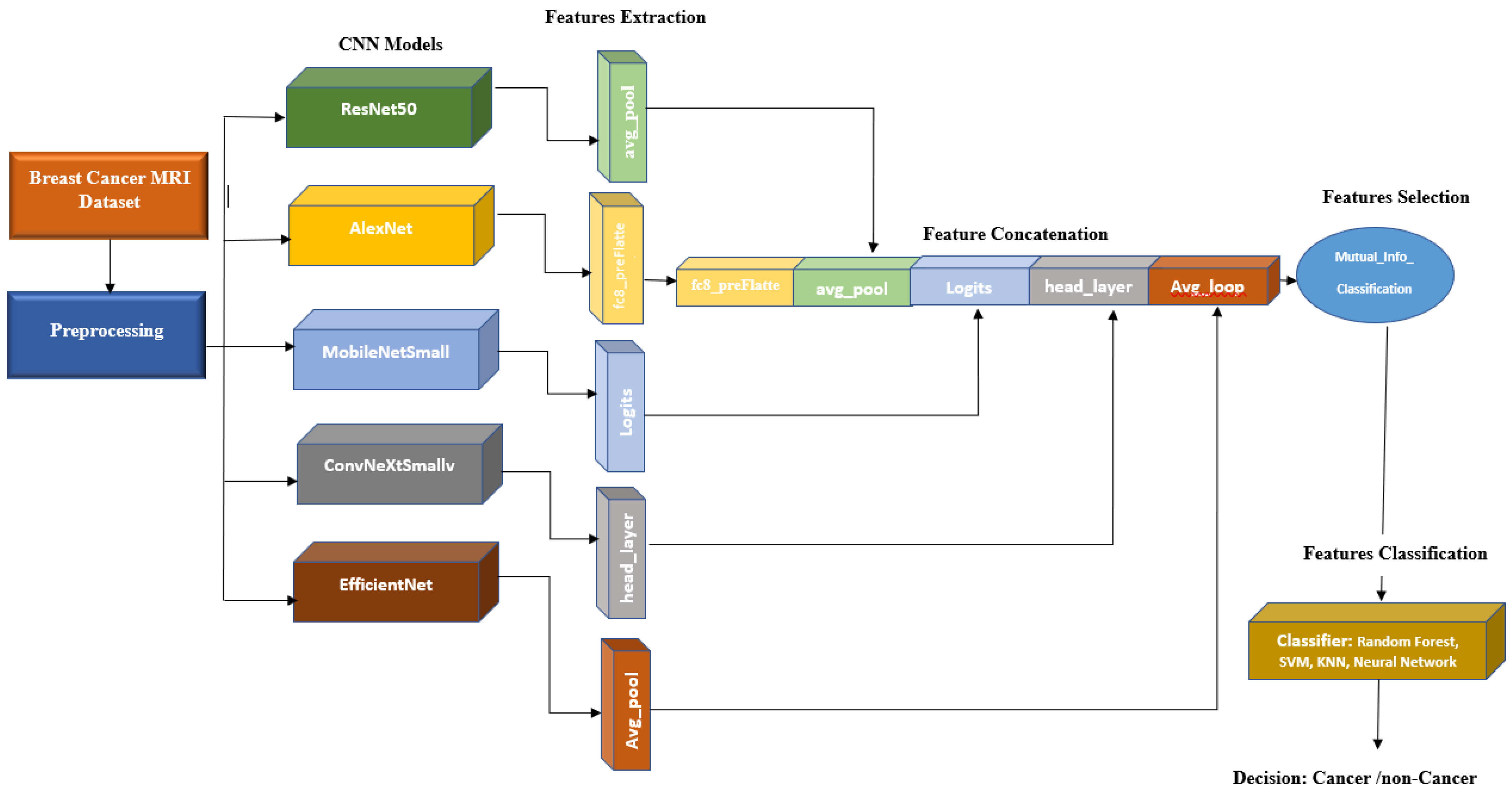
The proposed system uses five base models, namely Alexnet, Resnet50, MobileNetSmall, ConvNeXtSmall, and EfficienNet, whose features are concatenated and extracted for optimal classification with a neural network (NN) model. This approach demonstrated its capability to enhance the accuracy of BC classification.
2. Materials and Methods
2.1. Datasets
- The main dataset for this project is the radiological society of north america (RSNA) dataset from a recent Kaggle competition [22]. The dataset contains 54,713 images in dicom format from roughly 11,000 patients. For each patient, there are at least four images from different laterality and views. For each subject, two different views CC and MLO, and images from left and right laterality were provided. The images are of various sizes and formats, including jpeg and jpeg2000, and different types, such as monochrome-1 and monochrome-2. The dataset provides additional features some of which can be used for classification purposes: age, implant, BIRADS, and density. We base our work on this dataset, but since this dataset is new, it has not been used in any published research yet. Hence, for comparison purposes, we use two other well-known datasets MIAS and DDSM. This dataset is imbalanced as only 2 percent of the images are from cancer patients, which makes any classification method biased. To compensate for this, we use all positive cases and only 2320 images from negative cases. Figure 1 depicts two sample images from this dataset for cancer and normal cases.
- The mammographic image analysis society (MIAS) [23] dataset is a well-known and widely used dataset for the development and evaluation of CAD systems for BC detection. It consists of 322 mammographic images, with each image accompanied by a corresponding ground truth classification of benign or malignant tumors. The dataset is particularly valuable for researchers interested in developing machine learning algorithms for BC detection, as it includes examples of both normal and abnormal mammograms, as well as a range of breast densities and lesion types. Figure 2 depicts two sample images from this dataset for cancer and normal cases.
- The digital database for screening mammography (DDSM) [24] includes 55,890 images, of which 14% are positive, and the remaining 86% are negative. Images were tiled into 598 × 598 tiles, which were then resized to 299 × 299. A subset of this dataset which is for positive cases and is called CBIS-DDSM, has been annotated and the region of interest has been extracted by experts. In this research, we do not use the CBIS-DDSM and use the original DDSM dataset as we are classifying the images from normal subjects and cancer patients. Figure 3 depicts two sample images from this dataset for cancer and normal cases. Table 1 summarizes these three datasets.
2.2. Models
- AlexNet [25] is a deep CNN architecture that was introduced in 2012 and achieved a breakthrough in computer vision tasks such as image classification. It consists of eight layers, including five convolutional layers and three fully connected layers. The first convolutional layer uses a large receptive field to capture low-level features such as edges and textures, while subsequent layers use smaller receptive fields to capture increasingly complex and abstract features. AlexNet was the first deep network to successfully use the rectified linear unit (ReLU) activation functions, which have since become a standard activation function in deep learning. It also used dropout regularization to prevent overfitting during training. AlexNet’s success on the ImageNet dataset, which contains over one million images, demonstrated the potential of deep neural networks for image recognition tasks and paved the way for further advances in the field of computer vision.
- ResNet50 [26] is a deep CNN architecture that uses residual connections to enable learning from very deep architectures without suffering from the vanishing gradient problem. It consists of 50 layers, including convolutional layers, batch normalization layers, ReLU activation functions, and fully connected layers. ResNet50 also uses a skip connection that bypasses several layers in the network, allowing it to effectively learns both low-level and high-level features.
- EfficientNet [27] is a family of deep CNN architectures that were introduced in 2019 and have achieved state-of-the-art performance on a range of computer vision tasks. EfficientNet uses a compound scaling method to simultaneously optimize the depth, width, and resolution of the network, allowing it to achieve high accuracy while maintaining computational efficiency. EfficientNet consists of a backbone network that extracts features from input images and a head network that performs the final classification. The backbone network uses a combination of mobile inverted bottleneck convolutional layers and squeeze-and-excitation (SE) blocks to capture both spatial and channel-wise correlations in the input. The head network uses a combination of global average pooling and fully connected layers to perform the final classification.
- MobileNet [28] is a deep learning architecture suitable for efficient and accurate analysis of medical images, specifically in the context of BC diagnosis. With its emphasis on computational efficiency, MobileNet can effectively extract features from mammography images, enabling the detection of subtle patterns or abnormalities associated with breast cancer. By utilizing depthwise separable convolutions, MobileNet optimizes memory consumption and computational load, making it ideal for resource-constrained environments. The integration of the ReLU6 activation function further enhances efficiency and compatibility with medical imaging devices. Overall, MobileNet offers a valuable solution for BC analysis, providing accurate results while operating efficiently on limited computational resources.
- ConvNeXt [29] is an architecture that enhances the representational capacity of CNNs by leveraging parallel branches to capture diverse and complementary features, leading to improved performance on challenging visual recognition tasks. It has demonstrated excellent performance on various computer vision tasks, including image classification, object detection, and semantic segmentation. Its ability to capture complex relationships between features has made it a popular choice for tasks requiring a high-level understanding of visual data.
3. Proposed Method
In this paper, we propose a method based on the extraction and concatenation of features obtained from various CNN models. The extracted features are then reduced such that only good features are selected and then used for the classification of normal and cancerous images. Figure 4 illustrates the block diagram of the proposed system. As one can see, the images from different datasets are first preprocessed, and then features are extracted through different CNN models. The extracted features are reduced and then classified into two: cancer and no cancer. The details for each block are as follows:
- A.
- Preprocessing: In this research, the images obtained from various datasets exhibit variations in sizes and resolutions.
- 1.
- Normalization:The RSNA dataset consists of images in various formats, including 12 and 16 bits per pixel. Additionally, it has two different photometric interpretations known as MONOCHROME1 and MONOCHROME2. The former represents grayscale images with ascending pixel values from bright to dark, while the latter represents grayscale images with ascending pixel values from dark to bright. To ensure consistency within the RSNA dataset, we convert all MONOCHROME1 images to MONOCHROME2.In order to standardize the pixel values across the RSNA dataset, intensity normalization is performed. This involves scaling the pixel values to the range of 0 to 255, which is equivalent to 8 bits per pixel. By applying this normalization process, the pixel values across the dataset become more consistent and comparable.On the other hand, the DDSM and MIAS datasets already have pixel values within the range of 0 to 255, eliminating the need for additional normalization. Therefore, the pixel values in these datasets are deemed suitable, and no further adjustment is required.
- 2.
- Region of Interest Selection:To select the region of interest, we initially apply a global thresholding method to the image. Subsequently, we extract the contour of the largest object present in the image, which corresponds to the breast area. Utilizing this contour, we generated a mask that enables us to crop the image and isolate the specific region of interest for further analysis.
- 3.
- Image Alignment:In breast cancer datasets, there are two distinct laterality categories: left and right. To enhance consistency and improve accuracy in analysis, we align all laterality labels to the left side. This process involves horizontally flipping all left breast images to create a uniform orientation throughout the datasets. By standardizing the laterality representation, we ensure a consistent and reliable dataset for further research and analysis purposes.
- B.
- Feature extraction: For feature extraction, we exploit the features computed by pre-trained CNN models described in Section 2.2. For each model, the features are extracted from the last layer before the last fully connected (FC) layer as the output of the final FC layer has been trained for 1000 classes of the ImageNet dataset, and hence, we skip this layer and extract the features from the last layer before the final FC layer. Table 2 depicts the layer before the final FC layer and the number of features extracted for each CNN model used in this paper.
- C.
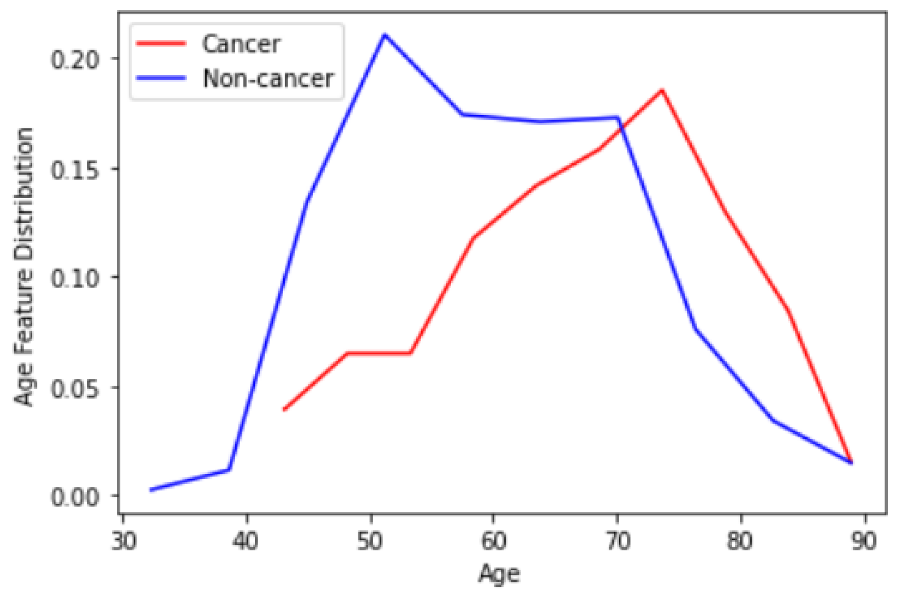
- Feature concatenation: The 1-dimensional (1D) features extracted in the previous step are concatenated to form a single 1D feature vector. Note that for each CNN model, we have extracted features from two different views CC and MLO. Hence, 10 1D vectors are concatenated here. This forms a vector with a size of 18,384 For the RSNA dataset that we use as the basis of our research, we have an additional useful feature for the patient age. Figure 5 depicts the distribution of the age feature provided by the RSNA dataset for both cancer and non-cancer subjects. As can be observed, age can also be considered a valuable feature. We can also simply normalize and add age to our feature vector to have 18,385 features in total.
- D.
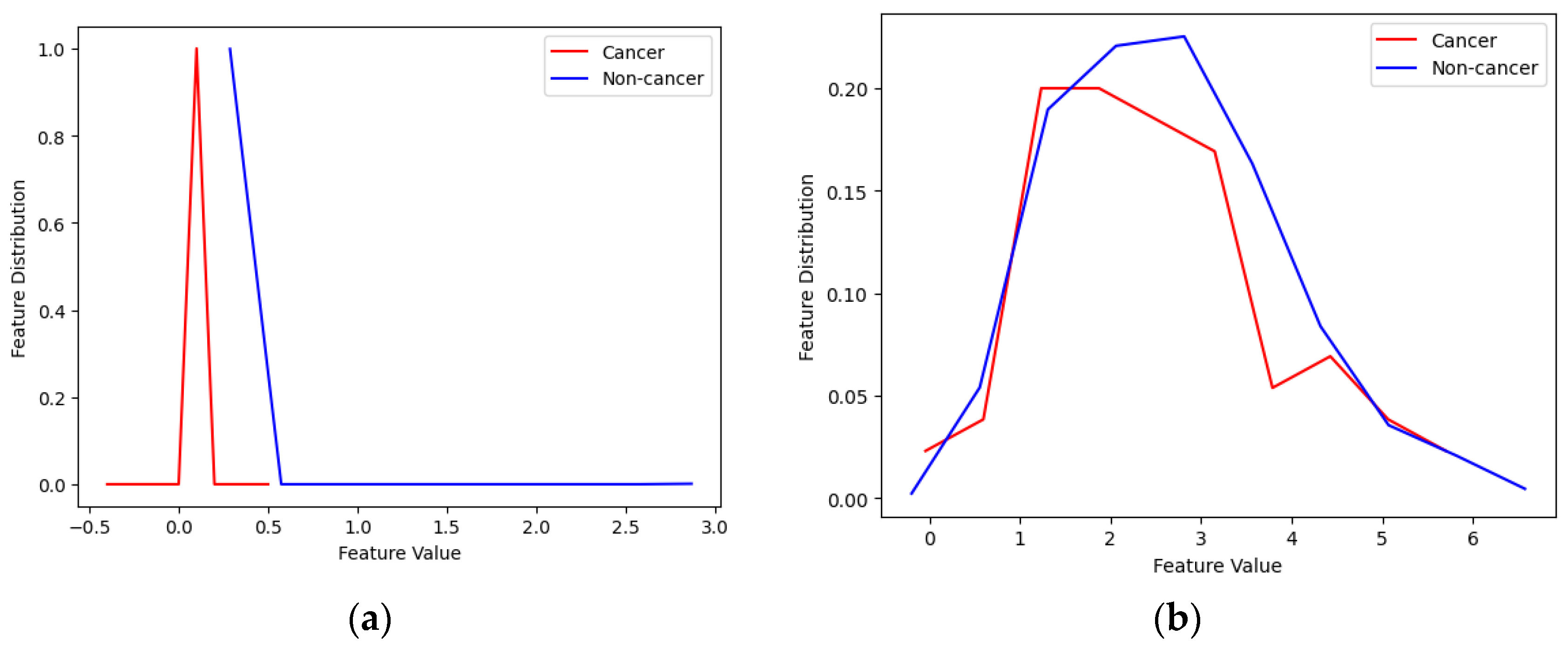
- Feature selection: The majority of the features are redundant and do not carry any useful information and only increase the complexity of the system. Figure 6 illustrates 2 samples of good and weak features. As one can see from the figure, in the case of weak features, the distribution of the feature for normal and cancerous subjects are similar showing that there is no useful information in this feature and the calculated mutual information between them is zero. For the case of good features, normal and cancerous subjects have obviously different distributions showing that these features carry useful information, although small, that can improve the performance of classifiers used in the next step. To compute mutual information we use the method in [30]. We empirically found a 0.02 threshold gives us the best results. Note that we have also adopted feature selection based on mutual information empirically and after using various feature selection methods. The number of features for each dataset before and after feature selection is presented in Table 3.
- E.
- Feature classification: After selecting the best features, we need to classify them. For this purpose, we tried multiple machine learning algorithms such as k-NN, random forest (RF), SVM, and NN. In our study, we utilize an RF algorithm with specific parameters to enhance breast cancer detection. We construct an ensemble of 100 trees, setting the minimum number of samples required to split a node as 2. Additionally, we limit the maximum number of features considered for each tree to 5 and the maximum tree depth to 4. These parameter settings are chosen to optimize the performance of our model and improve the accuracy of breast cancer detection in our X-ray image datasets.In our SVM classifier implementation, we utilize a linear kernel and set the regularization parameter “C” to a value of 1. The linear kernel allows us to learn a linear decision boundary, while the “C” parameter balances the trade-off between training accuracy and the complexity of the decision boundary.In the k-NN classifier, we set k = 5, and for the NN classifier, we used two fully connected (FC) layers with a hidden layer including 96 neurons and a single-neuron classification layer. For the classification layer, we use a sigmoid activation function that classifies non-cancer cases from cancerous ones.
4. Results and Discussion
This section showcases the results obtained from the three datasets introduced in Section 2.1 using the models described in Section 2.2, as well as a combination of all datasets as illustrated in Figure 4. For each dataset, we employed k-fold cross-validation with k = 10. This means that the method was trained and tested 10 times, with 90% of the data allocated for training and 10% for testing in each iteration.
4.1. Evaluation Metrics [31]
To assess the performance of our experiments, we utilize various evaluation metrics.
- True positives (TP): Instances where the predicted class and actual class are both positive. This indicates that the classifier accurately classified the instance with a positive label.
- False positives (FP): Instances where the predicted class is positive but the actual class is negative. This means that the classifier incorrectly classified the instance with a positive label. In the context of breast abnormality classification, an FP response corresponds to a type I error according to statisticians. For example, it could refer to a calcification image being classified as a mass lesion or a benign mass lesion being classified as a malignant mammogram in the diagnosis.
- True negatives (TN): Instances where the predicted class and actual class are both negative. This indicates that the classifier correctly classified the instance with a negative label.
- False negatives (FN): Instances where the predicted class is negative but the actual class is positive. This means that the classifier incorrectly classified the instance with a negative label. In the context of breast abnormality classification, an FN response is considered a type II error. For instance, it could refer to a mass mammogram being classified as calcification or a malignant mass lesion being classified as a benign mammogram in the diagnosis. Type II errors are particularly significant in their consequences.
- Accuracy: This metric represents the overall number of correctly classified instances. In the case of the abnormality classifier, accuracy signifies the correct classification of image patches containing either mass or calcification. Similarly, accuracy shows the correct classification of image patches as either malignant or benign in the pathology classifier.
- Sensitivity or Recall: This metric represents the proportion of positive image patches that are correctly classified. In the abnormality type classifier, sensitivity indicates the fraction of image patches that are truly mass lesions and are correctly classified. Similarly, the abnormality pathology classifier shows the fraction of truly malignant image patches that are correctly classified. Given the significance of type II errors, this metric is valuable for evaluating performance.
- Precision: This metric reflects the proportion of positive predictions that are correctly categorized. It is calculated using the following formula:
- F1 Score: This measure combines the impact of recall and precision using the harmonic mean, giving equal penalties to extreme values. It is commonly calculated using the formula:
4.2. Performance Evaluation of the Proposed Model for Different Classifiers
Table 4 presents a comparison of performance metrics for different CNN models using the RSNA dataset. Among the individual CNN models, EfficientNet consistently outperforms the other models in terms of accuracy, sensitivity, precision, AUC, and F-Score. Its superior performance can be attributed to its architecture, which enables it to capture relevant features and make accurate predictions on the RSNA dataset. EfficientNet proves to be the most effective choice among the individual models for accurately classifying medical images in the RSNA dataset. From the last row of the table, one can see that the proposed concatenation scheme, significantly improves all performance metrics, for instance, the achieved accuracy is 6 percent more than the best CNN model, i.e., EfficientNet.
Table 5 presents a summary of the results obtained using the kNN classifier with k = 5. The findings indicate a significant decline in performance compared to the NN model. Specifically, without feature concatenation, the highest accuracy is achieved with AlexNet, which is 8 percent lower than the accuracy of the same model with the NN classifier, and 13 percent lower than the best-performing EfficientNet model with the NN classifier. Additionally, the accuracy of the concatenated model is also 14 percent lower compared to the concatenated model with the NN classifier.
Table 6 displays the results obtained from the RF classifier. It demonstrates that the accuracy of the concatenated Model is equivalent to that of the KNN classifier, but falls short compared to the NN. Among the individual models, EfficientNet exhibits the most favorable performance metrics, while mobileNetSmall exhibits the least favorable performance.
Table 7 displays the results of the proposed method using the SVM classifier. It is evident from the table that SVM exhibits the lowest accuracy among all four investigated methods. Specifically, the accuracy of the SVM-based method is 19 percent lower than that of the NN-based method. Furthermore, in comparison to the KNN and RF-based systems, the accuracy of the concatenated model decreased by 5 percent.
4.3. Comparison of the Proposed System with State-of-the-Art Methods
Based on the findings presented in Table 4, Table 5, Table 6 and Table 7, it is evident that the NN classifier achieves the highest level of performance. Therefore, we employed the suggested approach using the NN classifier as the benchmark to compare it with the existing methods.
To the best of our knowledge, the RSNA dataset has not been utilized in any previously published papers. Consequently, for the purposes of this section, we conducted a comparison of our proposed model against existing methods using the MIAS and DDSM datasets and summarized the results in Table 8.
Upon examining Table 8, it is evident that our proposed model has exhibited superior performance compared to state-of-the-art algorithms in terms of accuracy and sensitivity across both the MIAS and DDSM datasets. While the method described in [32] demonstrated slightly better precision for the MIAS dataset, our algorithm outperformed it in the remaining two performance metrics.
4.4. Cross-Dataset Validation
So far, we have trained and tested the proposed method on the same dataset. However, it is crucial to evaluate the ability of a model trained on one dataset to perform well on different datasets or images collected from diverse machines and under varying image collection standards. In this subsection, we assess the performance of our method when trained on one of three datasets: RSNA, MIAS, and DDSM, and subsequently tested on images from a different dataset. The results of these experiments are summarized in Table 9.
Since the RSNA dataset comprises images of various types and resolutions, cross-validating it with another dataset yields slightly lower performance metrics. Specifically, when the method is trained on either the MIAS or DDSM dataset and tested on RSNA images, the achieved performance is slightly reduced. Figure 1 visually depicts the resemblance between RSNA and MIAS images compared to RSNA and DDSM images, further supporting the observation that cross-validation between RSNA and MIAS datasets leads to higher accuracy compared to cross-validation involving RSNA and DDSM datasets. These findings are also supported by the results presented in Table 9.
5. Conclusions
We have developed a novel method to address the accurate diagnosis of breast cancer in mammography images. Our approach involves the extraction and selection of features from multiple pre-trained CNN models, followed by classification using various machine learning algorithms: kNN, SVM, RF, and NN. The results obtained for different datasets demonstrate the effectiveness of our proposed scheme.
Our findings indicate that the NN-based classifier yielded the best performance in our experiments. Notably, we achieved impressive accuracies of 92%, 94.5%, and 96% for the RSNA, MIAS, and DDASM datasets, respectively. These results surpass those of existing methods, underscoring the superiority of our approach in terms of accuracy and sensitivity.
In terms of future work, we envision several directions to enhance our method. Firstly, exploring advanced deep learning techniques, such as attention mechanisms, could further improve the model’s performance. Secondly, investigating the integration of additional clinical and genomic data could potentially enhance the accuracy and predictive capabilities of our system. Lastly, conducting rigorous validation on larger-scale datasets from multiple healthcare institutions would provide more robust evidence of the method’s effectiveness and generalizability.
Author Contributions
Z.J. provided, and cleaned the dataset, and implemented the algorithms, and Z.J and E.K. performed experiments and wrote the paper. E.K. edited the paper. All authors have read and agreed to the published version of the manuscript.
Funding
The research received no external funding.
Data Availability Statement
Not applicable.
Acknowledgments
We would like to thank Morteza Golzan and Hamideh Mehri for their support.
Conflicts of Interest
The authors declare no conflict of interest.
References
- Ferlay, J.; Colombet, M.; Soerjomataram, I.; Parkin, D.M.; Piñeros, M.; Znaor, A.; Bray, F. Cancer statistics for the year 2020: An overview. Int. J. Cancer 2021, 149, 778–789. [Google Scholar] [CrossRef]
- Lei, S.; Zheng, R.; Zhang, S.; Wang, S.; Chen, R.; Sun, K.; Zeng, H.; Zhou, J.; Wei, W. Global patterns of breast cancer incidence and mortality: A population-based cancer registry data analysis from 2000 to 2020. Cancer Commun. 2021, 41, 1183–1194. [Google Scholar] [CrossRef]
- Marks, J.S.; Lee, N.C.; Lawson, H.W.; Henson, R.; Bobo, J.K.; Kaeser, M.K. Implementing recommendations for the early detection of breast and cervical cancer among low-income women. Morb. Mortal. Wkly. Rep. Recomm. Rep. 2000, 49, 35–55. [Google Scholar]
- Du-Crow, E. Computer-Aided Detection in Mammography; The University of Manchester: Manchester, UK, 2022. [Google Scholar]
- Evans, A.; Trimboli, R.M.; Athanasiou, A.; Balleyguier, C.; Baltzer, P.A.; Bick, U.; Herrero, J.C.; Clauser, P.; Colin, C.; Cornford, E.; et al. Breast ultrasound: Recommendations for information to women and referring physicians by the European Society of Breast Imaging. Insights Imaging 2018, 9, 449–461. [Google Scholar] [CrossRef] [Green Version]
- Schueller, G.; Schueller-Weidekamm, C.; Helbich, T.H. Accuracy of ultrasound-guided, large-core needle breast biopsy. Eur. Radiol. 2008, 18, 1761–1773. [Google Scholar] [CrossRef] [PubMed]
- Shi, X.; Liang, C.; Wang, H. Multiview robust graph-based clustering for cancer subtype identification. IEEE/ACM Trans. Comput. Biol. Bioinform. 2022, 20, 544–556. [Google Scholar] [CrossRef]
- Wang, H.; Jiang, G.; Peng, J.; Deng, R.; Fu, X. Towards Adaptive Consensus Graph: Multi-view Clustering via Graph Collaboration. IEEE Trans. Multimed. 2022, 1–13. [Google Scholar] [CrossRef]
- Wang, H.; Wang, Y.; Zhang, Z.; Fu, X.; Zhuo, L.; Xu, M.; Wang, M. Kernelized multiview subspace analysis by self-weighted learning. IEEE Trans. Multimed. 2020, 23, 3828–3840. [Google Scholar] [CrossRef]
- Wang, H.; Yao, M.; Jiang, G.; Mi, Z.; Fu, X. Graph-Collaborated Auto-Encoder Hashing for Multi-view Binary Clustering. arXiv 2023, arXiv:2301.02484. [Google Scholar]
- Bai, J.; Posner, R.; Wang, T.; Yang, C.; Nabavi, S. Applying deep learning in digital breast tomosynthesis for automatic breast cancer detection: A review. Med. Image Anal. 2021, 71, 102049. [Google Scholar] [CrossRef]
- Li, Z.; Liu, F.; Yang, W.; Peng, S.; Zhou, J. A survey of convolutional neural networks: Analysis, applications, and prospects. IEEE Trans. Neural Netw. Learn. Syst. 2022, 33, 6999–7019. [Google Scholar] [CrossRef] [PubMed]
- Zuluaga-Gomez, J.; Al Masry, Z.; Benaggoune, K.; Meraghni, S.; Zerhouni, N. A CNN-based methodology for breast cancer diagnosis using thermal images. Comput. Methods Biomech. Biomed. Eng. Imaging Vis. 2021, 9, 131–145. [Google Scholar] [CrossRef]
- Eroğlu, Y.; Yildirim, M.; Çinar, A. Convolutional Neural Networks based classification of breast ultrasonography images by hybrid method with respect to benign, malignant, and normal using mRMR. Comput. Biol. Med. 2021, 133, 104407. [Google Scholar] [CrossRef] [PubMed]
- Huang, Q.; Yang, F.; Liu, L.; Li, X. Automatic segmentation of breast lesions for interaction in ultrasonic computer-aided diagnosis. Inf. Sci. 2015, 314, 293–310. [Google Scholar] [CrossRef]
- Huang, Q.; Huang, Y.; Luo, Y.; Yuan, F.; Li, X. Segmentation of breast ultrasound image with semantic classification of superpixels. Med. Image Anal. 2020, 61, 101657. [Google Scholar] [CrossRef]
- Zhou, J.; Luo, L.; Dou, Q.; Chen, H.; Chen, C.; Li, G.; Jiang, Z.; Heng, P. Weakly supervised 3D deep learning for breast cancer classification and localization of the lesions in MR images. J. Magn. Reson. Imaging 2019, 50, 1144–1151. [Google Scholar] [CrossRef]
- Yurttakal, A.H.; Erbay, H.; Ikizceli, T.; Karaçavuş, S. Detection of breast cancer via deep convolution neural networks using MRI images. Multimed. Tools Appl. 2019, 79, 15555–15573. [Google Scholar] [CrossRef]
- Rahman, A.S.; Belhaouari, S.B.; Bouzerdoum, A.; Baali, H.; Alam, T.; Eldaraa, A.M. Breast mass tumor classification using deep learning. In Proceedings of the 2020 IEEE International Conference on Informatics, IoT, and Enabling Technologies (ICIoT), Doha, Qatar, 2 February 2020; pp. 271–276. [Google Scholar]
- Sun, L.; Wang, J.; Hu, Z.; Xu, Y.; Cui, Z. Multi-view convolutional neural networks for mammographic image classification. IEEE Access 2019, 7, 126273–126282. [Google Scholar] [CrossRef]
- Heravi, E.J.; Aghdam, H.H.; Puig, D. Classification of Foods Using Spatial Pyramid Convolutional Neural Network. InCCIA 2016, 288, 163–168. [Google Scholar] [CrossRef]
- Carr, C.; Kitamura, F.; Partridge, G.; Kalpathy-Cramer, J.; Mongan, J.; Andriole, K.; Lavender Vazirabad, M.; Riopel, M.; Ball, R.; Dane, S.; et al. RSNA Screening Mammography Breast Cancer Detection, Kaggle 2022. Available online: https://kaggle.com/competitions/rsna-breast-cancer-detection (accessed on 1 December 2022).
- Suckling, J.; Parker, J.; Dance, D.; Astley, S.; Hutt, I.; Boggis, C.; Ricketts, I.; Stamatakis, E.; Cerneaz, N.; Kok, S.; et al. Mammographic Image Analysis Society (Mias) Database v1. 21. Available online: https://www.repository.cam.ac.uk/handle/1810/250394 (accessed on 2 February 2023).
- Heath, M.; Bowyer, K.; Kopans, D.; Kegelmeyer, P.; Moore, R.; Chang, K.; Munishkumaran, S. Current status of the digital database for screening mammography. Digit. Mammogr. Nijmegen 1998, 1998, 457–460. [Google Scholar] [CrossRef]
- Krizhevsky, A.; Sutskever, I.; Hinton, G.E. Imagenet classification with deep convolutional neural networks. Commun. ACM 2017, 60, 84–90. [Google Scholar] [CrossRef] [Green Version]
- He, K.; Zhang, X.; Ren, S.; Sun, J. Deep residual learning for image recognition. In Proceedings of the IEEE Conference on Computer Vision and Pattern Recognition 2016, Las Vegas, NV, USA, 27–30 June 2016; pp. 770–778. [Google Scholar]
- Tan, M.; Le, Q. Efficientnetv2: Smaller models and faster training. In Proceedings of the International Conference on Machine Learning, PMLR, Virtual Event, 1 July 2021; pp. 10096–10106. [Google Scholar]
- Howard, A.G.; Zhu, M.; Chen, B.; Kalenichenko, D.; Wang, W.; Weyand, T.; Andreetto, M.; Adam, H. Mobilenets: Efficient convolutional neural networks for mobile vision applications. arXiv 2017, arXiv:1704.04861. [Google Scholar]
- Liu, Z.; Mao, H.; Wu, C.Y.; Feichtenhofer, C.; Darrell, T.; Xie, S. A convnet for the 2020s. In Proceedings of the IEEE/CVF Conference on Computer Vision and Pattern Recognition 2022, New Orleans, LA, USA, 19–20 June 2022; pp. 11976–11986. [Google Scholar]
- Ross, B.C. Mutual Information between Discrete and Continuous Data Sets. PLoS ONE 2014, 9, e87357. [Google Scholar] [CrossRef] [PubMed]
- Azour, F.; Boukerche, A. An efficient transfer and ensemble learning based computer aided breast abnormality diagnosis system. IEEE Access 2022, 11, 21199–21209. [Google Scholar] [CrossRef]
- Rampun, A.; Scotney, B.W.; Morrow, P.J.; Wang, H.; Winder, J. Breast density classification using local quinary patterns with various neighbourhood topologies. J. Imaging 2018, 4, 14. [Google Scholar] [CrossRef] [Green Version]
- Vijayarajeswari, R.; Parthasarathy, P.; Vivekanandan, S.; Basha, A.A. Classification of mammogram for early detection of breast cancer using SVM classifier and Hough transform. Measurement 2019, 146, 800–805. [Google Scholar] [CrossRef]
- Arafa, A.A.A.; El-Sokary, N.; Asad, A.; Hefny, H. Computer-aided detection system for breast cancer based on GMM and SVM. Arab. J. Nucl. Sci. Appl. 2019, 52, 142–150. [Google Scholar] [CrossRef] [Green Version]
- Diaz, R.A.; Swandewi, N.N.; Novianti, K.D. Malignancy determination breast cancer based on mammogram image with k-nearest neighbor. In Proceedings of the 2019 1st International Conference on Cybernetics and Intelligent System (ICORIS), Denpasar, Indonesia, 22 August 2019; Volume 1, pp. 233–237. [Google Scholar]
- Agrawal, S.; Rangnekar, R.; Gala, D.; Paul, S.; Kalbande, D. Detection of breast cancer from mammograms using a hybrid approach of deep learning and linear classification. In Proceedings of the 2018 International Conference on Smart City and Emerging Technology (ICSCET), Mumbai, India, 5 January 2018; pp. 1–6. [Google Scholar]
- Li, B.; Ge, Y.; Zhao, Y.; Guan, E.; Yan, W. Benign and malignant mammographic image classification based on convolutional neural networks. In Proceedings of the 2018 10th International Conference on Machine Learning and Computing, New York, NY, USA, 26 February 2018; pp. 247–251. [Google Scholar]
- Platania, R.; Shams, S.; Yang, S.; Zhang, J.; Lee, K.; Park, S.J. Automated breast cancer diagnosis using deep learning and region of interest detection (bc-droid). In Proceedings of the 8th ACM International Conference on Bioinformatics, Computational Biology, and Health Informatics, Boston, MA, USA, 20 August 2017; pp. 536–543. [Google Scholar]
- Swiderski, B.; Kurek, J.; Osowski, S.; Kruk, M.; Barhoumi, W. Deep learning and non-negative matrix factorization in recognition of mammograms. In Proceedings of the Eighth International Conference on Graphic and Image Processing (ICGIP 2016), Tokyo, Japan, 8 February 2017; Volume 10225, pp. 53–59. [Google Scholar]
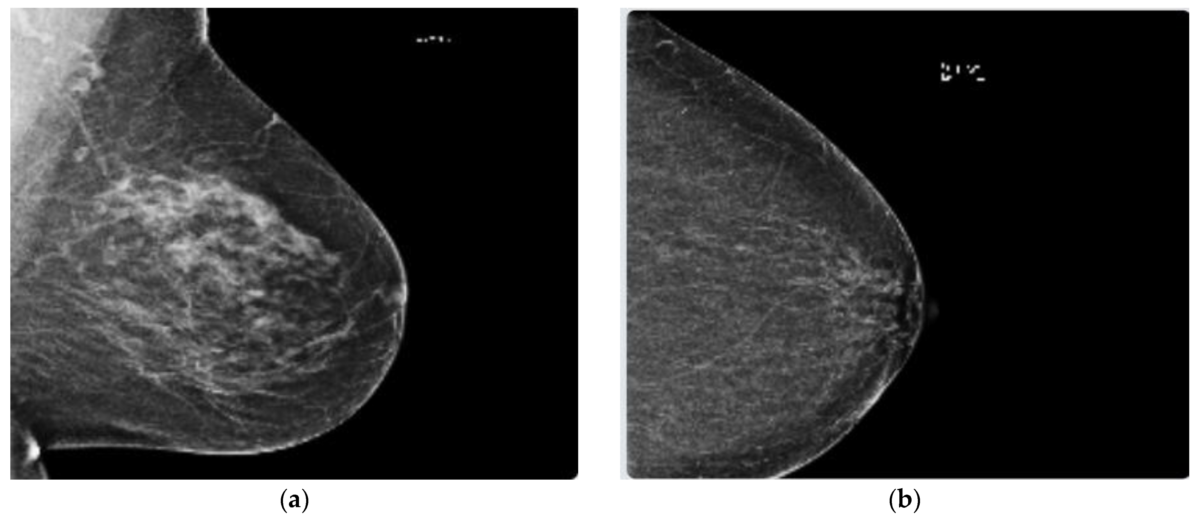
Figure 1.
These figures show two sample images from the RSNA dataset for (a) a cancerous, and (b) a normal subject.
Figure 1.
These figures show two sample images from the RSNA dataset for (a) a cancerous, and (b) a normal subject.

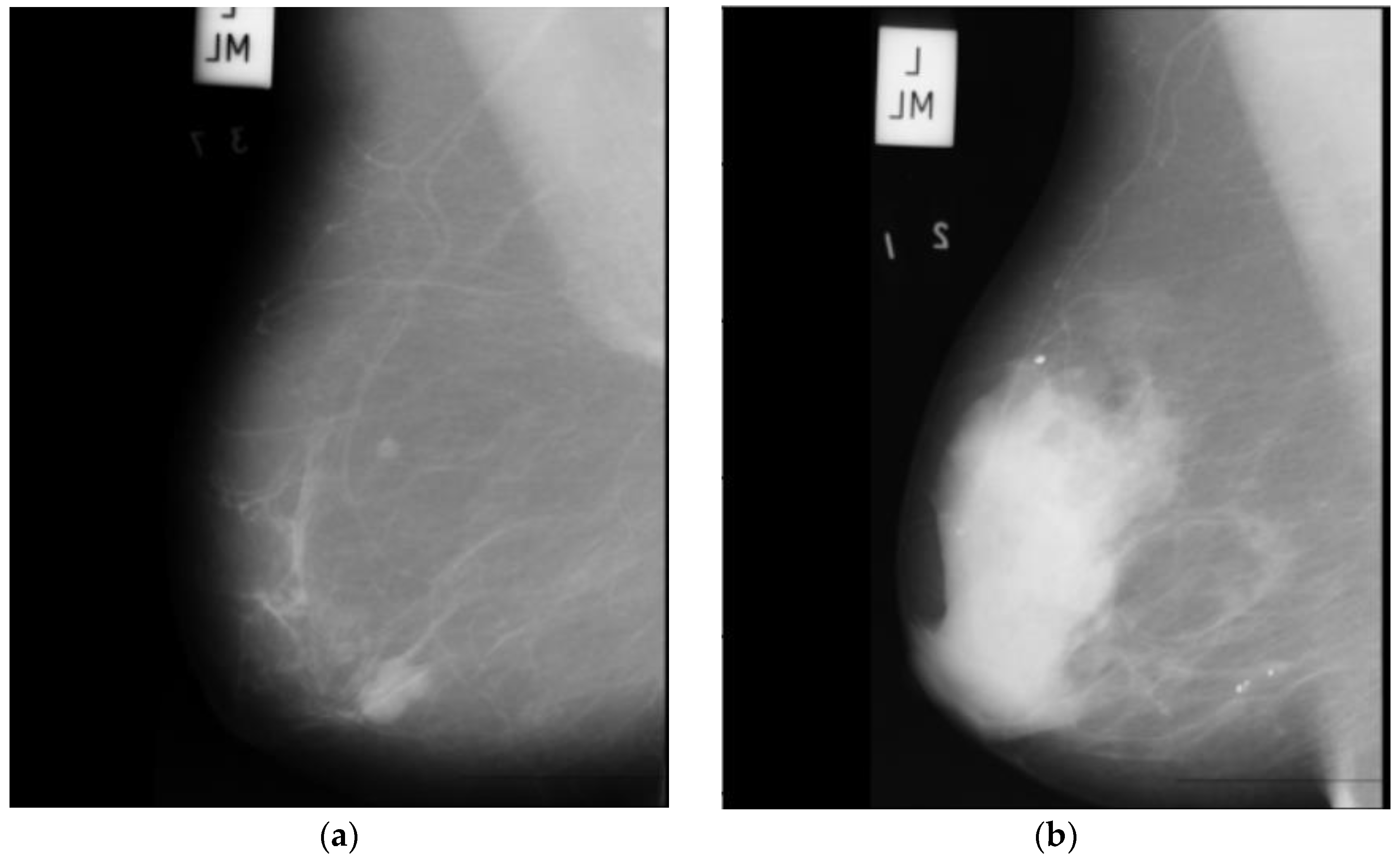
Figure 2.
These figures show two sample images from the MIAS dataset for (a) cancerous, and (b) normal subjects.
Figure 2.
These figures show two sample images from the MIAS dataset for (a) cancerous, and (b) normal subjects.

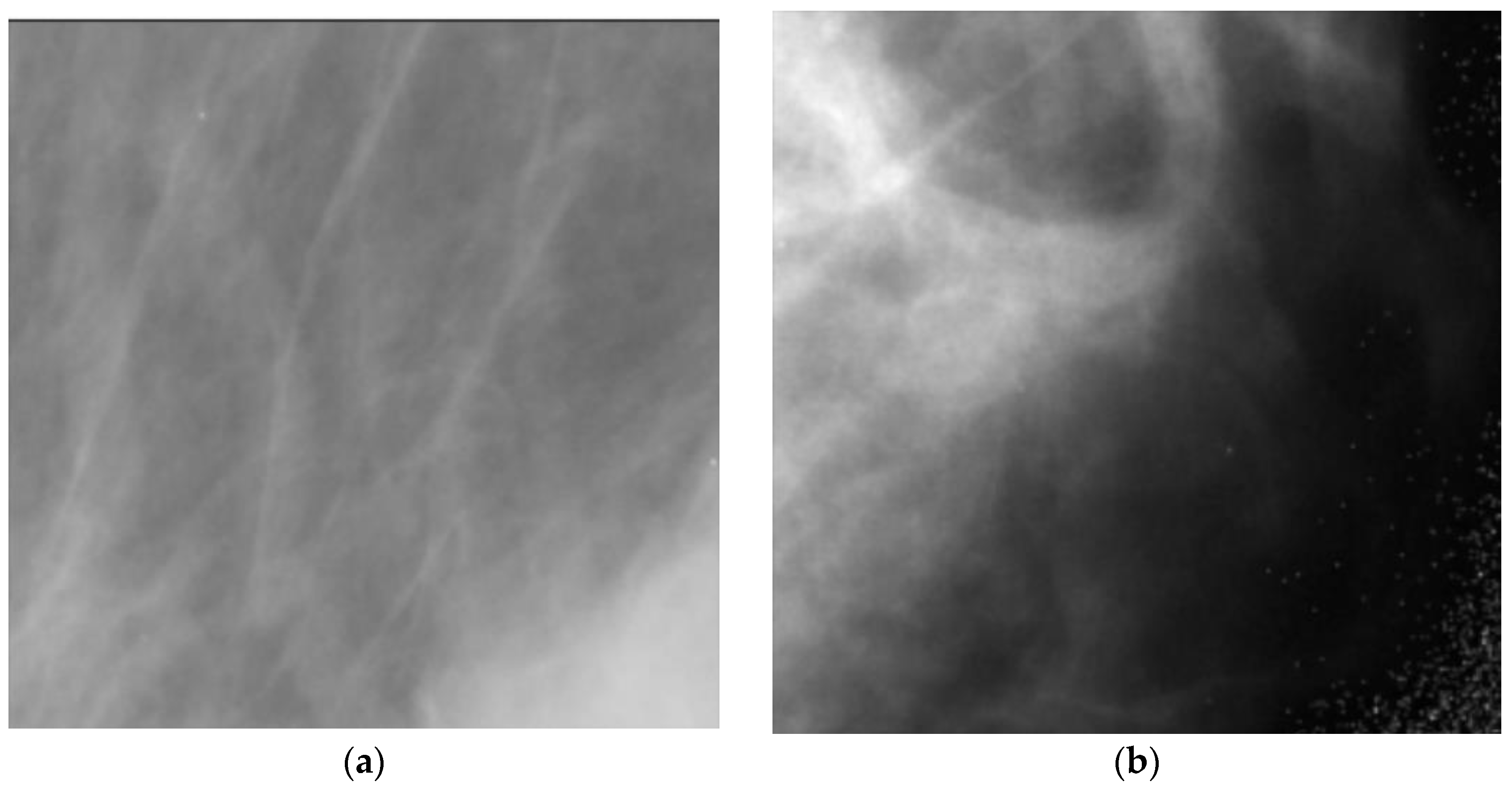
Figure 3.
These figures show two sample images from the DDSM dataset for (a) cancerous and (b) normal subjects.
Figure 3.
These figures show two sample images from the DDSM dataset for (a) cancerous and (b) normal subjects.

Figure 4.
Block diagram of the proposed system.

Figure 5.
This figure shows the distribution of age for cancer and noncancer subjects in the RSNA dataset.
Figure 5.
This figure shows the distribution of age for cancer and noncancer subjects in the RSNA dataset.

Figure 6.
These figures show distributions of (a) a good feature and (b) a weak feature extracted using a pre-trained CNN model. for cancer and noncancer subjects in the DDSM dataset. The mutual information computed for these two features is 0.035 and zero, respectively.
Figure 6.
These figures show distributions of (a) a good feature and (b) a weak feature extracted using a pre-trained CNN model. for cancer and noncancer subjects in the DDSM dataset. The mutual information computed for these two features is 0.035 and zero, respectively.


Table 1.
This table shows the description of three datasets.
| Dataset | Number of Images | Image Types | Image Size |
|---|---|---|---|
| RSNA | 54,713 | Variable | Variable |
| MIAS | 322 | PGM | 1024 × 1024 |
| DDSM | 55,890 | JPEG | 598 × 598 |
Table 2.
This table shows the CNN models used in the proposed method along with the layer name where the features have been extracted and the number of features extracted from each model.
Table 2.
This table shows the CNN models used in the proposed method along with the layer name where the features have been extracted and the number of features extracted from each model.
| CNN Models | Layer Name 1 | Number of Features |
|---|---|---|
| ResNet50 | avg_pool | 2048 |
| AlexNet | fc8_preflatten | 4096 |
| MobileNetSmall | Logits | 1000 |
| ConvNeXtSmall | head_layer | 768 |
| EfficientNet | avg_pool | 1280 |
1 Layer’s names have been taken from TensorFlow models.
Table 3.
The total number of features obtained from each dataset before and after feature selection.
Table 3.
The total number of features obtained from each dataset before and after feature selection.
| Dataset | Before Feature Selection | After Feature Selection |
|---|---|---|
| RSNA | 18,385 1 | 452 |
| MIAS | 9192 | 212 |
| DDSM | 9192 | 206 |
1 RSNA dataset provides two views for each subject and one additional feature for age.
Table 4.
Performance comparison of the proposed method for different CNN models and Concat. Model with the NN classifier for RSNA dataset.
Table 4.
Performance comparison of the proposed method for different CNN models and Concat. Model with the NN classifier for RSNA dataset.
| CNN Models | Acc | Sn | Pr | AUC | F-Score |
|---|---|---|---|---|---|
| AlexNet | 81% | 84% | 87% | 0.82 | 0.86 |
| Resnet50 | 84% | 90% | 86% | 0.89 | 0.88 |
| MobileNetSmall | 77% | 85% | 81% | 0.81 | 0.83 |
| ConvNexSmall | 79% | 87% | 83% | 0.83 | 0.85 |
| EfficientNet | 86% | 92% | 88% | 0.92 | 0.90 |
| Concat. Model | 92% | 96% | 92% | 0.96 | 0.94 |
Table 5.
Performance comparison of the proposed method for different CNN models and Concat. Model with the kNN classifier for RSNA dataset.
Table 5.
Performance comparison of the proposed method for different CNN models and Concat. Model with the kNN classifier for RSNA dataset.
| CNN Models | Acc | Sn | Pr | AUC | F-Score |
|---|---|---|---|---|---|
| AlexNet | 73% | 70% | 72% | 0.70 | 0.71 |
| Resnet50 | 72% | 75% | 71% | 0.73 | 0.73 |
| MobileNetSmall | 64% | 71% | 67% | 0.68 | 0.69 |
| ConvNexSmall | 66% | 74% | 70% | 0.71 | 0.72 |
| EfficientNet | 71% | 78% | 74% | 0.76 | 0.76 |
| Concat. Model | 78% | 81% | 79% | 0.82 | 0.80 |
Table 6.
Performance comparison of the proposed method for different CNN models and Concat. Model with the RF classifier for RSNA dataset.
Table 6.
Performance comparison of the proposed method for different CNN models and Concat. Model with the RF classifier for RSNA dataset.
| CNN Models | Acc | Sn | Pr | AUC | F-Score |
|---|---|---|---|---|---|
| AlexNet | 71% | 67% | 69% | 0.68 | 0.68 |
| Resnet50 | 69% | 70% | 67% | 0.71 | 0.68 |
| MobileNetSmall | 60% | 67% | 63% | 0.64 | 0.65 |
| ConvNexSmall | 62% | 69% | 65% | 0.67 | 0.67 |
| EfficientNet | 73% | 74% | 70% | 0.75 | 0.72 |
| Concat. Model | 78% | 79% | 77% | 0.80 | 0.78 |
Table 7.
Performance comparison of the proposed method for different CNN models and Concat. Model with the SVM classifier for RSNA dataset.
Table 7.
Performance comparison of the proposed method for different CNN models and Concat. Model with the SVM classifier for RSNA dataset.
| CNN Models | Acc | Sn | Pr | AUC | F-Score |
|---|---|---|---|---|---|
| AlexNet | 62% | 61% | 63% | 0.62 | 0.62 |
| Resnet50 | 64% | 66% | 63% | 0.65 | 0.64 |
| MobileNetSmall | 60% | 63% | 59% | 0.60 | 0.61 |
| ConvNexSmall | 62% | 65% | 61% | 0.63 | 0.63 |
| EfficientNet | 68% | 70% | 66% | 0.68 | 0.68 |
| Concat. Model | 73% | 75% | 72% | 0.74 | 0.73 |
Table 8.
Performance comparison of our proposed model vs. methods using the MIAS and DDSM datasets.
| Method | Dataset | Number of Images | ACC | Sn | Pr |
|---|---|---|---|---|---|
| SVM & Hough [32] | MIAS & InBreast | 322&206 | 86.13% | 80.67% | 92.81% |
| LQP & SVM [33] | MIAS | 95 | 94% | NA | NA |
| GMM & SVM [34] | Mini-MIAS dataset | 90 | 92.5% | NA | NA |
| KNN [35] | Mini-MIAS | 120 | 92% | NA | NA |
| Voting Classifier [36] | MIAS | 322 | 85% | NA | NA |
| CNN-4d [37] | Mini-MIAS | 547 | 89.05% | 90.63% | 83.67% |
| CNN [38] | DDSM | 10,480 | 93.5% | NA | NA |
| CNNs [39] | DDSM | 11,218 | 85.82% | 82.28% | 86.59% |
| Our Method + NN | RSNA | 54,713 | 92% | 96% | 92% |
| Our Method + NN | MIAS | 322 | 94.5% | 96.32% | 91.80% |
| Our Method + NN | DDSM | 55,890 | 96% | 94.70% | 97% |
Table 9.
Performance of the proposed model with cross-dataset validation, i.e., trained and tested with different datasets.
Table 9.
Performance of the proposed model with cross-dataset validation, i.e., trained and tested with different datasets.
| Train Dataset | Test Dataset | ACC | Sn | Pr |
|---|---|---|---|---|
| RSNA | MIAS | 79.13% | 82.67% | 80.81% |
| RSNA | DDSM | 74% | 77.50% | 76% |
| MIAS | RSNA | 76.5% | 78.80% | 78% |
| MIAS | DDSM | 80.70% | 82% | 82.80% |
| DDSM | RSNA | 72% | 75.50% | 76% |
| DDSM | MIAS | 79% | 80% | 79.87% |
Disclaimer/Publisher’s Note: The statements, opinions and data contained in all publications are solely those of the individual author(s) and contributor(s) and not of MDPI and/or the editor(s). MDPI and/or the editor(s) disclaim responsibility for any injury to people or property resulting from any ideas, methods, instructions or products referred to in the content. |
© 2023 by the authors. Licensee MDPI, Basel, Switzerland. This article is an open access article distributed under the terms and conditions of the Creative Commons Attribution (CC BY) license (https://creativecommons.org/licenses/by/4.0/).
Share and Cite
MDPI and ACS Style
Jafari, Z.; Karami, E. Breast Cancer Detection in Mammography Images: A CNN-Based Approach with Feature Selection. Information 2023, 14, 410. https://0-doi-org.brum.beds.ac.uk/10.3390/info14070410
AMA Style
Jafari Z, Karami E. Breast Cancer Detection in Mammography Images: A CNN-Based Approach with Feature Selection. Information. 2023; 14(7):410. https://0-doi-org.brum.beds.ac.uk/10.3390/info14070410
Chicago/Turabian StyleJafari, Zahra, and Ebrahim Karami. 2023. "Breast Cancer Detection in Mammography Images: A CNN-Based Approach with Feature Selection" Information 14, no. 7: 410. https://0-doi-org.brum.beds.ac.uk/10.3390/info14070410
Note that from the first issue of 2016, this journal uses article numbers instead of page numbers. See further details here.