Article

Interpreting Disentangled Representations of Person-Specific Convolutional Variational Autoencoders of Spatially Preserving EEG Topographic Maps via Clustering and Visual Plausibility

Artificial Intelligence and Cognitive Load Lab, The Applied Intelligence Research Centre, School of Computer Science, Technological University Dublin, D07 EWV4 Dublin, Ireland
*
Author to whom correspondence should be addressed.
Submission received: 11 July 2023 / Revised: 26 August 2023 / Accepted: 30 August 2023 / Published: 4 September 2023
(This article belongs to the Special Issue Advances in Explainable Artificial Intelligence)

Abstract

:
Dimensionality reduction and producing simple representations of electroencephalography (EEG) signals are challenging problems. Variational autoencoders (VAEs) have been employed for EEG data creation, augmentation, and automatic feature extraction. In most of the studies, VAE latent space interpretation is used to detect only the out-of-order distribution latent variable for anomaly detection. However, the interpretation and visualisation of all latent space components disclose information about how the model arrives at its conclusion. The main contribution of this study is interpreting the disentangled representation of VAE by activating only one latent component at a time, whereas the values for the remaining components are set to zero because it is the mean of the distribution. The results show that CNN-VAE works well, as indicated by matrices such as SSIM, MSE, MAE, and MAPE, along with SNR and correlation coefficient values throughout the architecture’s input and output. Furthermore, visual plausibility and clustering demonstrate that each component contributes differently to capturing the generative factors in topographic maps. Our proposed pipeline adds to the body of knowledge by delivering a CNN-VAE-based latent space interpretation model. This helps us learn the model’s decision and the importance of each component of latent space responsible for activating parts of the brain.

1. Introduction

Electroencephalography (EEG) is a method of recording brain activity (electrical potentials) using electrodes placed on the scalp [1]. It is generally known that EEG signals carry important information in the frequency, temporal, and spatial domains. EEG signals have been regularly used to diagnose a variety of mental disorders. However, analysis is difficult and decisions are tough to accept due to the low amplitude, complex collecting settings, and substantial noise [2]. EEG examines voltage variations in the order of microvolts caused by ionic currents within the neurons of the brain. Brain mapping is a neuroscience approach for exploring the advancement of understanding the structure and function of the human brain. EEG topography mapping (EEG topo-map) is a neuroimaging approach that uses a visual–spatial depiction to map the EEG signal. The EEG data from the electrodes is collected and processed into EEG topographical maps. The EEG topo-map visualises raw EEG data of voltage or power amplitude [3]. Some studies, for example, have converted EEG signals into topographic power head maps in order to preserve spatial information [4,5,6]. Topographic maps, on the other hand, are frequently redundant and contain significantly interpolated data between electrode locations. Many machine learning and deep learning algorithms have used temporal- and frequency-domain features to classify EEG signals. On the other hand, only a few studies combine the spatial and temporal dimensions of the EEG signal. As a result, it is difficult to build efficient algorithms using features based on prior information. Therefore, the 2D convolutional neural network (CNN) is utilised to learn EEG features across diverse mental tasks without previous knowledge [7]. There are many techniques that have been employed to reduce their dimensionality and automatically learn essential features. The tensor-decomposition-based dimensionality reduction algorithm, transforms the CNN input tensor into a concise set of slices [8]. Another popular dimensionality reduction technique is spatial filtering. The performance of various spatial filtering techniques has been evaluated on the test set. These spatial filtering techniques extract EEG nonstationarity features that cause model accuracy to deteriorate even after 30 min of resting. These feature changes had varying effects on the spatial filtering algorithms chosen [9]. They also rely on a restricted number of channels because they restrict us from investigating the neural plausibility of the derived features in greater depth. EEG is referred to as a nonstationary signal since it fluctuates from subject to subject, and even from one recording session to the next for the same person [10,11]. The generative network accepts random noise from a certain distribution (e.g., Gaussian) and aims to generate synthetic data that is identical to real data. Since generative networks are sensitive to image generation, significant features from EEG signals are retrieved as images and used as the model’s input [12]. An autoencoder (AE) is a deep learning neural network architecture that uses unsupervised learning to learn efficient features without using labelled input. These features, also known as latent spaces, are often lower in dimension than the original input and are utilised to reconstruct it with high fidelity [13]. During the encoding stage, a neural network uses a set of encoding parameters θ = { W , b } to translate the input x to a hidden representation y = f θ ( x ) = s ( W x + b ) . Secondly, by using decoding parameters θ = W , b , the hidden representation y is mapped to the reconstructed vector z = g θ ( y ) = s W y + b [14].
A variational autoencoder (VAE) is a form of autoencoder that creates a probabilistic model of the input sample and then reconstructs it using that model. As a result, VAEs can be employed to generate synthetic data [15]. VAEs have shown a wide application with electroencephalographic (EEG) signals [16,17,18]. VAEs employ convolutional processes on input topographic maps to learn prominent high-level features that are lower in dimension, as shown in Figure 1. These high-level features are more portable because they do not require a large amount of digital memory to be stored. This lower level also includes useful and prominent representations of EEG data that can be used for a variety of reasons.
In the recent literature, the VAE has been employed for EEG data creation, augmentation, denoising, and automatic feature extraction. However, little research has been conducted into how the VAE model arrives at its conclusions.
The primary contribution of this study is to understand the significance of each latent space component of a convolutional variational autoencoder (CNN-VAE) trained with spatially preserved EEG topographic maps which influence the generative factors in EEG topographic maps. This can be achieved by interpreting the disentangled representation of a VAE by activating just one latent component at a time and setting the remaining components to zero, because it represents the distribution’s mean. Disentangling the representation of CNN-VAE provides meaningful visualisations that aid in understanding which component of latent space is responsible for capturing which region of brain activation in EEG topographic maps. The learned CNN-VAE model is assessed by computing the SNR for actual and reconstructed EEG signals when the decoder network is trained with all latent components. Furthermore, it is also assessed by computing the average and channel-wise correlation values between the actual and the reconstructed signals with one active component at a time.
The proposed approach advances in the field of explainable artificial intelligence (XAI) by interpreting and disentangling the representation of VAE to understand the model’s conclusion. In this study, the goal is to tackle the research problem of learning the importance of each latent component of VAE trained with spectral topographic EEG maps.Therefore, the research question being addressed is:
RQ: Can a convolutional variational autoencoder (CNN-VAE) trained with spectral topographic maps and interpreting its disentangled representation disclose its decision?
The rest of the work is organised as follows. Section 2 investigates related work on VAE latent space representation and interpretation, whereas Section 3 describes an empirical study and its methodology to answer the above research question. Section 4 presents the experimental results and findings. Section 5 represents the discussion. Finally, Section 6 concludes the manuscript by describing the contribution to the body of knowledge and highlighting future work directions.

2. Related Work

Traditional autoencoders (AEs) aim to learn prominent latent representations from unlabelled input while ignoring irrelevant features. As a result, the reconstructed data will be identical to the input data. Variational autoencoders (VAEs) were recently proposed as an effective extension of AEs, for modelling a dataset’s probability distribution and learning a latent space, usually of a lower dimension, without explicit supervision [19]. In detail, this latent space is not composed of a fixed vector, but of a mixture of distributions. A VAE allows us to encode an input x to a latent vector z = E n c o d e r ( x ) q ( z x ) using an encoder network, and then use another network to decode this latent vector z back to a shape that is as close as possible to the original input data x ¯ = Decoder ( z ) p ( x z ) . In other words, the goal is to maximise the marginal log-likelihood of each observation in x, and the VAE reconstruction loss L r e c to the negative anticipated log-likelihood of the observations x [19], as in the following:
L r e c = E q ( z x ) [ log p ( x z ) ]
The performance of machine learning algorithms is often dependent on data representation because it can entangle and disguise many explanatory aspects of variations hidden beneath the data. VAE-based latent space analysis and decoding of EEG signals are important since they can precisely define and determine the relevant latent features [20]. Therefore, the VAE model gives a closed-form latent space representation of the distribution underlying the input data, which is ideal for unsupervised learning in order to understand the significance of each latent component in terms of capturing the number of true generative factors. In order to understand the VAE’s decision, its disentangled representation must be interpreted and visualised. The following sub-section examines previous research on the interpretation of latent space representations.

2.1. Interpreting the VAE Disentangling Representations

This section includes a literature review on interpreting and disentangling the latent space of a VAE to understand its decision toward reconstruction capacity. The learned representation must be interpreted because the latent component is simple to understand. Therefore, the models based on latent representations, such as VAE, have recently emerged as powerful tools in this domain since their latent space can encode crucial hidden variables in the input data. A VAE requires the typical Gaussian distribution as a prior in the latent space; because all codes tend to follow the same prior they frequently suffer from posterior collapse [21]. The disentanglement is a condition of the latent space in which each latent variable is sensitive to changes in only one feature while being insensitive to changes in the others [13]. There are several ways to learn a disentangled latent space [13]. However, approaches that exploit the VAE structure are of special importance to our work. The disentangled latent variables have been applied successfully in a variety of applications, including face recognition [22], video prediction [23], and anomaly detection [24]. Another recent study uses VAE for anomaly detection, in which the latent space is partially disentangled and interpreted, with a few latent variables capturing the majority of the feature’s information and others encoding little information. As a result, the degree to which the latent space representations are disentangled must be quantified [25]. The disentangled representation of the VAE is mostly interpreted to determine the components of latent space that influence the capture of artefacts in data. This method is based on determining the latent variable’s out-of-order distribution (OOD). This can be accomplished by calculating the KL divergence of the images [26]. This is the difference between the generated latent distribution and the standard normal distribution ( μ = 0 , σ = 1 ) . The researcher provides one such definition, defining it as the degree to which a latent dimension d D in a representation predicts a true generative component k K , with each latent dimension capturing no more than one generative factor [27]. Therefore, manually adjusting the latent space component of the VAE enables the user to examine how different latent values affected the outcome of the model [28]. The researcher also illustrated how a VAE model’s latent space might be made more explainable by utilising latent space regularisation to force some selected dimensions of the latent space to map to meaningful musical qualities. Furthermore, a user interface feedback loop is provided to allow individuals to edit the parameters of the latent space and see the results of these changes in real time [29]. In another study, an attribute-regularized VAE (AR-VAE) is used, which employs a new supervised training method to generate structured latent spaces in which specified attributes are compelled to be embedded along specific dimensions of the latent space. The resulting latent spaces are simply interpretable and allow for the manipulation of individual properties via simple traversals along the regularised dimensions [30].

2.2. Interpretation of Latent Space for Cluster Analysis

Disentangling representations of generative adversarial networks (GANs) for clustering analysis have been intensively investigated to address the high-dimensionality issue associated with data. All latent components form a single large cluster, making them difficult to use for OOD or anomaly detection [26,31]. Therefore, the interpretation of latent space forms several smaller clusters of single latent variables if the features are independent. Such disentangled latent variables have been successfully used in several tasks such as face recognition [22] and anomaly detection. A new clustering approach called disentangling latent space clustering (DLS-clustering) directly learns cluster assignments using disentangled latent spacing without the use of extra clustering techniques. The latent space is split into two pieces by the disentangling process: discrete one-hot latent variables that are directly linked to categorical data and continuous latent variables that are linked to other sources of variation, which immediately results in clusters [32,33]. The researchers suggest an image-clustering method based on VAEs using a Gaussian mixture model (GMM) prior, with each component representing a cluster. The prior is learnt in conjunction with the posterior, which in turn learns a robust latent representation, resulting in an accurate clustering [34].
The interpretation of the VAE’s disentangling representation is commonly utilised to improve the accuracy of classification tasks and a wide range of applications such as face recognition, video prediction, and anomaly detection. It is also used in cluster analysis to discover the OOD latent variable that drives the artefacts. The majority of the disentangled representation is examined in order to identify the single OOD latent variable. As a result, it will be useful for anomaly detection. Understanding the decision of the VAE, on the other hand, requires knowledge of the contribution of all latent variables to the VAE’s reconstruction capacity. Understanding the significance of each latent component in spatially preserving EEG topographic maps via visual plausibility, clustering, and correlation values across the architecture’s input and output remains a challenge.

3. Materials and Methods

In this study, if CNN-VAE is trained with spatially preserved EEG topographic maps, it provides a similar SNR for actual and reconstructed EEG signals and a higher and more positive correlation across the input and output of the architecture. Additionally, interpretation and visualisation of the learnt latent space representation provide knowledge of how well each latent component contributes to capturing the number of true generative factors in EEG topographic maps via clustering and visual plausibility. The detailed design of this research is illustrated in Figure 2, and the following sections describe its components.

3.1. Dataset

DEAP: The DEAP dataset was chosen because it contains multi-channel EEG recordings with a large number of participants and tasks. EEG data were collected from 32 persons who watched 40 one-minute music video clips [35]. Following a 60-s music clip, each participant was asked to rate a video. Each film was scored on a 1–9 scale for dominance, like/dislike, valence, familiarity, and arousal. The standard 10–20 systems were applied with the following 32 electrode positions: ‘Fp1’, ‘AF3’, ‘F7’, ‘F3’, ‘FC1’, ‘FC5’, ‘T7’, ‘C3’, ‘CP1’, ‘CP5’, ‘P7’, ‘P3’, ‘Pz’, ‘PO3’, ‘O1’, ‘Oz’, ‘O2’, ‘PO4’, ‘P4’, ‘P8’, ‘CP6’, ‘CP2’, ‘C4’, ‘T8’, ‘FC6’, ‘FC2’, ‘F4’, ‘F8’, ‘AF4’, ‘Fp2’, ‘Fz’, ‘Cz’. Pre-processing comprised signal re-sampling at 128 Hz and a band-pass frequency filter that operated in the 1–50 Hz range.

3.2. EEG Topographic Head Maps Generation

Raw EEG signals were used in this stage to build spatially preserving EEG topographic maps. Before creating topographic maps, empirical tests were carried out to determine the best size of the topographic map that preserves spatial information about brain activation. This was performed by converting 3D to 2D polar to Cartesian coordinates and computing Euclidian distances between each channel in 2D polar to Cartesian coordinates as well as in 2D interpolated topographic map channel indexes. The results reveal that an image shape of 40 × 40 is the best form, with the smallest average difference between the electrode placements of 3D to 2D polar to Cartesian coordinates and 2D topographic map channel indexes. In addition, a 40 × 40 empty (with zeros) topographic map and a 2D edgeless image from the channel values are constructed. Finally, this 2D map is interpolated to produce maps of size 40 × 40 , as illustrated in Figure 2B.

3.3. A Convolutional Variational Autoencoder

Following the creation of the topographic maps, a convolutional variational autoencoder (CNN-VAE) is built with the goal of converting input data into probability distribution parameters such as the mean and standard deviation of a Gaussian distribution. The CNN-VAE of the proposed pipeline can be considered general enough to be used in finding simpler representations of data for analysis because this method generates a continuous, organised latent space that provides salient features of the data without losing information [36]. The learnt latent space representation is the simple form of the data, its visualisation and interpretation help us to understand the model’s decision. The CNN-VAE design consists of the following elements:
  • The encoder is a neural network that takes a 40 × 40 tensor (as seen in Figure 2C) and defines the approximate posterior distribution Q ( Z x ) , where x is the input tensor and Z is the latent space. The network will create the mean and standard deviation parameters of a factorised Gaussian with the latent space dimension of 25 by simply expressing the distribution as a diagonal Gaussian. This latent space dimension is the minimal dimension that leads to the maximum reconstruction capacity of the input EEG images. A similar experiment has been conducted on the EEG image shape of 32 × 32 × 5 , where the latent dimension 28 is considered as the minimal dimension that leads to the maximum reconstruction capacity of the input and maximum utility for classification tasks [5]. This architecture (Figure 2C) is made up of three 2D convolutional layers, each followed by a max pooling layer to minimise the dimension of the feature maps. In each convolutional layer, ReLU is employed as the activation function.
  • The CNN-VAE decoder is a generative network that takes a latent space Z as input and returns the parameters for the observation’s conditional distribution P ( x Z ) (as illustrated in the right side of Figure 2C). In this experiment, there are 2 different ways to train the decoder network. One is training it with latent space, utilising all variable values. The other way is to train with latent space where only one variable is active and has the latent sampled value, and all other variable values are set to zero, because zero is the mean of the distribution for each variable in the latent space. Similarly to the encoder network, the decoder is made up of three 2D convolutional layers, each followed by an up-sampling layer to reconstruct the data to the shape of the original input. In each convolutional layer, ReLU is employed as an activation function to regularise the neural network.
  • By sampling from the latent distribution described by the encoder’s parameters, the reparameterisation approach is utilised to provide a sample for the decoder. Because the backpropagation method in CNN-VAE cannot flow through a random sample node, sampling activities create a bottleneck. To remedy this, the reparameterisation technique is used to estimate the latent space Z using the decoder parameters plus one more, the ϵ parameter:
    Z = μ + σ ϵ
    where μ and σ are the mean and standard deviation of a Gaussian distribution, respectively, and ϵ is random noise used to maintain the stochasticity of Z. The latent space is now created using a function of μ , σ , and ϵ , allowing the model to backpropagate gradients in the encoder through μ and σ while retaining stochasticity through ϵ .
  • A loss function is used to optimise the CNN-VAEs in order to ensure that the latent space is both continuous and complete, the same as in our previous experiment [5]. Traditional VAE employs the binary cross-entropy loss function in conjunction with the Kullback–Leibler divergence loss, which is a measure of how two probability distributions differ from one another [37]. In this experiment, a new type of divergence known as maximum mean discrepancy (MMD) is introduced. The notion behind MMD is that two distributions are similar if and only if all of their moments are the same. As a result, KL-divergence is used to determine how “different” the moments of two distributions, p(z) and q(z) are from one another [38]. MMD can achieve this effectively using the kernel embedding trick:
    MMD ( p ( z ) q ( z ) ) = E p ( z ) , p z k z , z + E q ( z ) , q z k z , z 2 E p ( z ) , q z k z , z
    where k ( z , z ) can be any universal kernel, such as Gaussian. A kernel can be thought of as a function that compares the “similarity” of two samples. It has a high value when two samples are similar and a low value when they are dissimilar.
This CNN-VAE architecture is trained using a randomly picked 70% of 200,000 data samples from a single person, with the remaining 30% divided into validation and testing. To avoid overfitting, an early stopping strategy with a patience value of ten epochs is used, which indicates that training is stopped if the validation loss does not improve for ten consecutive epochs.

3.4. Clustering for Generative Factor Analysis

As shown in Figure 2C, the decoder network is trained with all of the values in the latent space and also trained with only one component value of the latent space, and the remaining latent variable is set to zero to test the impact of each component on capturing the generative factors. To examine the number of generative factors captured from each active latent component, the reconstructed EEG topographic map from the decoder of CNN-VAE is passed as an input to the k-means algorithm. The silhouette score is calculated to determine how well the reconstructed EEG topographic maps cluster with other topo maps. This score allows us to see how many clusters were created and how many patterns were learnt from each latent component, as shown in Figure 2D.

3.5. Reconstructed EEG Signals

The reconstructed EEG topo maps produced by each latent component are converted into EEG signals by reading only the pixel values corresponding to the 32 electrodes. Following that, for each channel in the signal, the correlation values between the actual and raw signals are computed. Furthermore, the average SNR for the test data is calculated as shown in Figure 2E.

3.6. Models Evaluation

To assess the performance of CNN-VAE, evaluation metrics must be defined. The reconstruction capacity of CNN-VAE is considered in two stages.

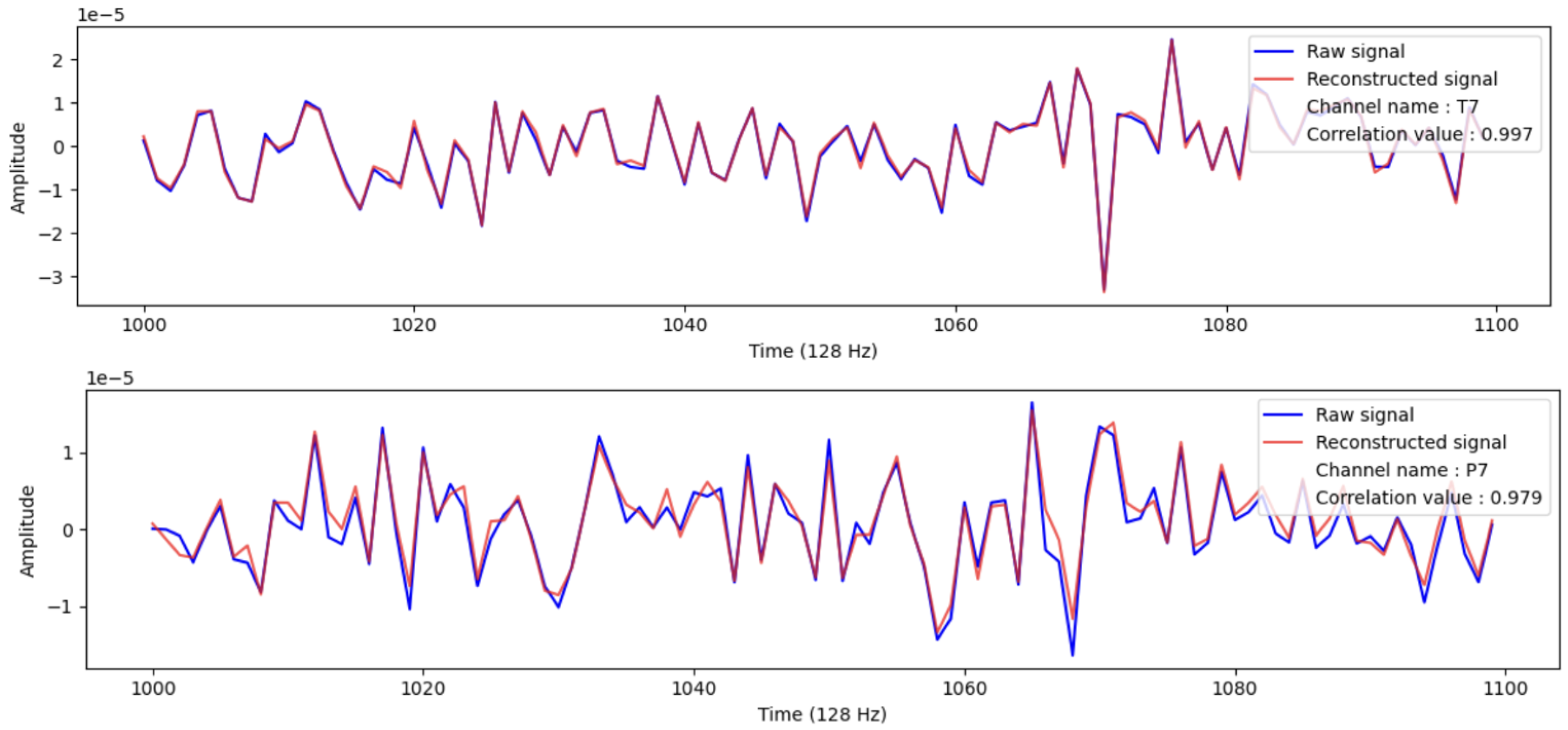
3.6.1. Evaluation of Reconstructed EEG Topographic Maps

The reconstruction capacity of the learnt CNN-VAE models was assessed against previously unseen testing data using the structural similarity index (SSIM), mean absolute error (MAE), and mean squared error (MSE).
  • SSIM: This is a perceptual metric that measures how much image quality is lost as a result of processing, including data compression. It is an index of structural similarity (in the real range [ 0 , 1 ] between two topographic maps (images) [39]). Values close to 1 indicate that the two topographic maps are very structurally similar, whereas values close to 0 indicate that the two images are exceptionally dissimilar and structurally different.
  • MAE: The average variance between the significant values in the dataset and the projected values in the same dataset is defined as the mean absolute error (MAE) [40].
  • MSE: This is defined as the mean (average) of the square of the difference between the actual and reconstructed values: a lower value indicates a better fit. In this case, the MSE involves the comparison, pixel by pixel, of the original and reconstructed topographic maps [39].

3.6.2. Evaluation of Reconstructed EEG Signals

  • Correlation coefficient: The correlation coefficient is a statistical measure of the strength of a two-variable linear relationship. Its values might range between −1 and 1. A positive correlation is represented by a number close to 1 [41].
  • Signal-to-noise ratio (SNR): An SNR is a measurement that compares the signal’s real information to the noise in the signal. It is defined as the ratio of the signal power to noise power in a signal [42].
    The formula for calculating an SNR is
    S N R = 20 log 10 S N
    S = ( signal ) 2 len ( signal ) N = ( noise ) 2 len ( noise )

4. Results

This section presents the findings of the following empirical studies. First, investigating the appropriate size for EEG topographic maps. Second, the CNN-VAE model’s performance in terms of reconstruction capacity for topographic images and EEG signals. Third, as indicated in Section 3.3, interpreting the disentangled representation of CNN-VAE utilising cluster analysis and coefficient of correlation across the input and output of the architecture.
All these empirical results help us find the impact of each VAE latent component on capturing the generative patterns of EEG signals.

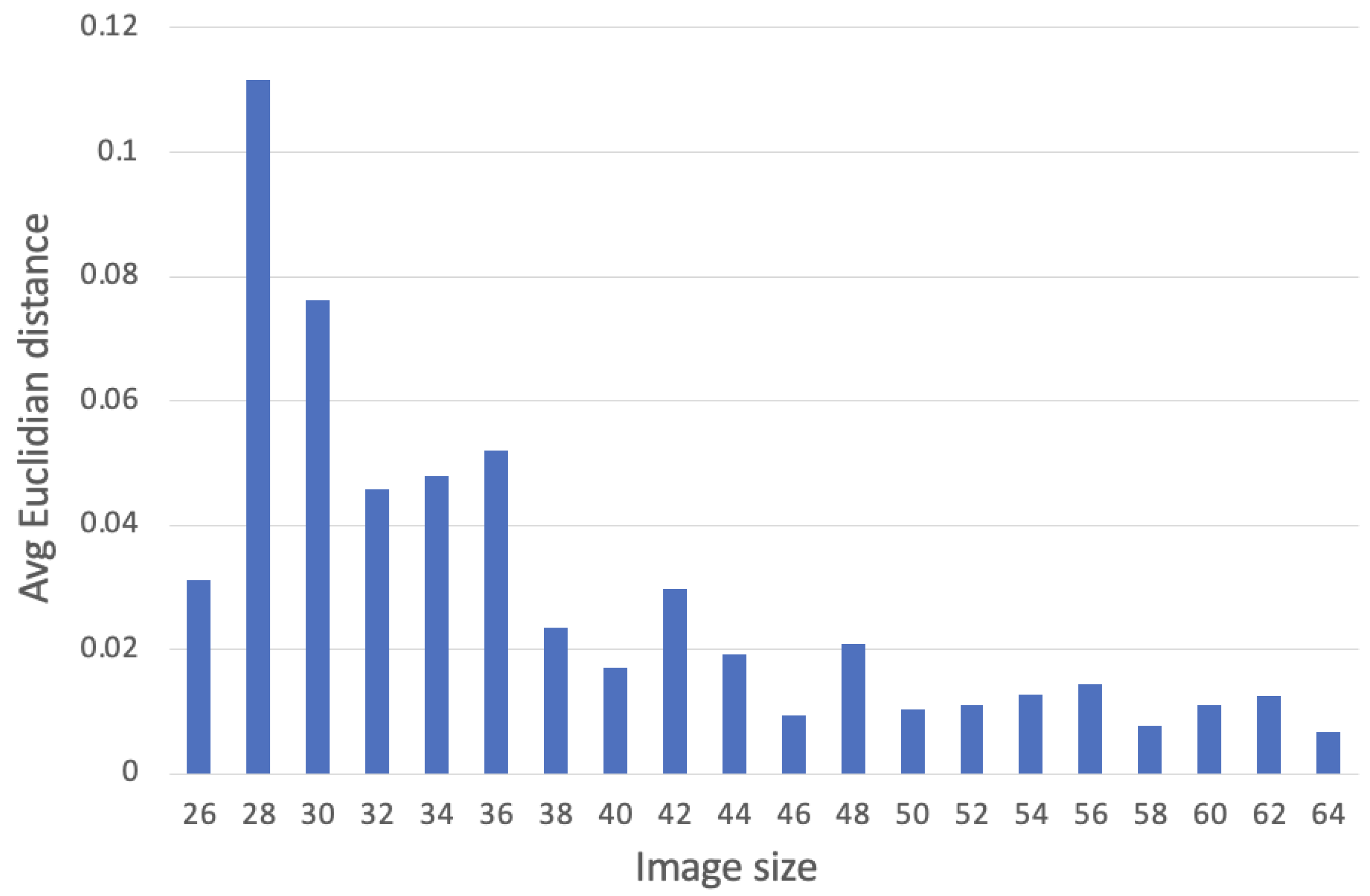
4.1. Examining the Size of the EEG Topographic Maps

Figure 3 depicts the average Euclidian distances calculated between each channel in 2D polar to Cartesian coordinates as well as in 2D interpolated topographic map channel indexes ranging in size from 26 × 26 to 64 × 64 . The results show that the image size 40 × 40 has the smallest average difference between electrode placements in 2D polar to Cartesian coordinates and 2D generated topo maps channel indexes. Additionally, increasing the image size has no effect on the average distance between the channels. These findings suggest that the image size of 40 × 40 retained the most spatial information of the EEG topo maps, which will be used as training data for the CNN-VAE in Section 3.3.

4.2. Reconstruction Capacity of CNN-VAE Model

Two scenarios are used to describe the CNN-VAE model’s reconstruction capabilities. One contains reconstructed EEG topography maps, while the other has reconstructed EEG signals. As described in Section 3.3, the decoder is trained with all latent variables as well as with only one active latent variable at a time, with the rest of the variables retained as zeros, because the empirical findings demonstrate that the mean of the latent space distribution for all latent components tends to be zero, shown in Figure A1, Appendix A. The distribution of the first four latent space components is depicted in Figure 4.
Table 1 shows the SSIM, MSE, MAE, and MAPE scores of the CNN-VAE models on unseen testing data, where this model was trained on 200,000 EEG topographic images with a latent space dimension of 25 and associated with one participant. It is feasible to observe that when all of the components in the latent space are used as input to the decoder, the SSIM value approaches one and the MSE, MAE, and MAPE values approach zero. This shows that CNN-VAE is functioning well in terms of topographic image reconstruction. Following that, the reconstructed EEG topo maps are transformed into EEG signals by reading only the pixel values corresponding to the 32 electrodes. The results demonstrate that all of the reconstructed signal channel data have a substantial positive correlation with the original raw data. Figure 5 depicts the signal from the T7 and P7 channels, as well as their correlation values with the original data’s channel values. This finding strongly confirms that the reconstructed signals are semantically similar to the original signal. Subsequently, the signal-to-noise ratio (SNR) for each channel of the original and reconstructed test data is computed. The result also shows that the reconstruction capacity of CNN-VAE is performing well because the SNR values are identical to each other when the decoder is trained with all latent components, shown in Figure 6.
Similar to the first scenario, the reconstruction capacity of CNN-VAE, where its decoder network is trained only with one latent component alternatively and the remaining 24 components are set to zero, is also investigated to examine the impact of each latent variable on generating the patterns in the EEG topo maps. The results show that each latent variable contributes differently to capturing the generated aspects in topo maps. Furthermore, the reconstruction capacity of CNN-VAE is evaluated using metrics such as SSIM, MSE, MAE, and MAPE, where the SSIM value approaches one and the MSE, MAE, and MAPE values approach zero, as shown in Table 1.

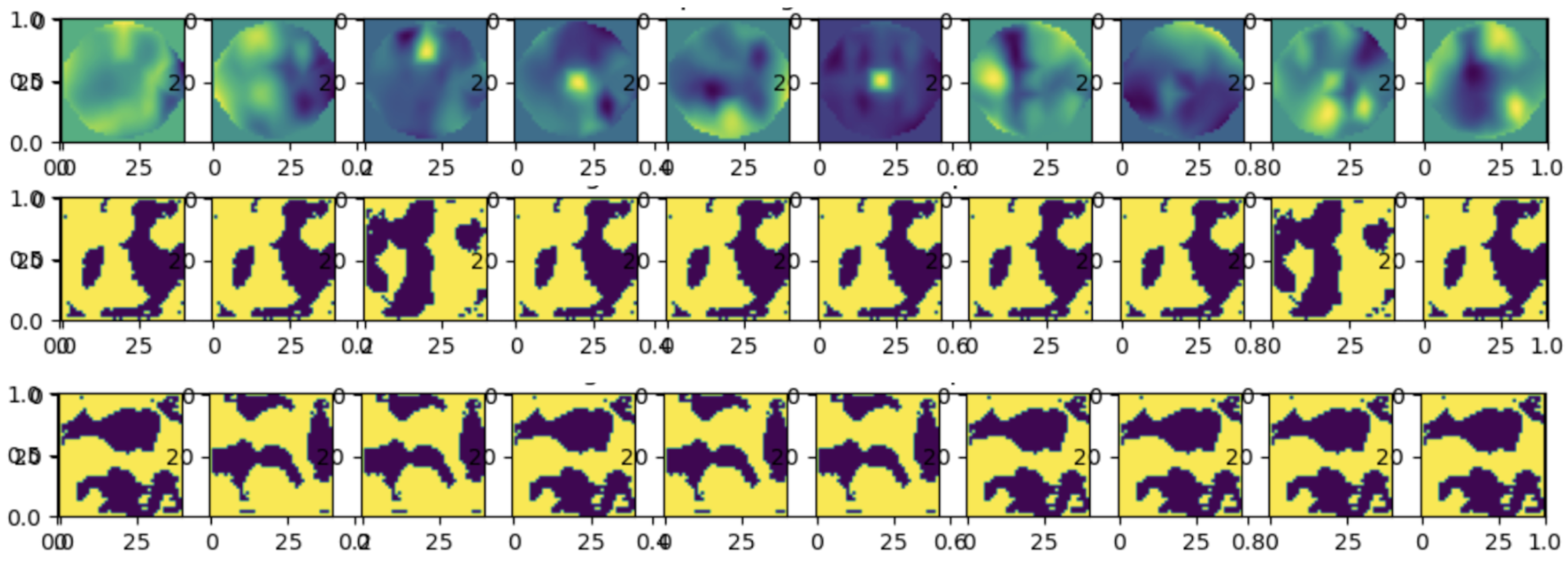
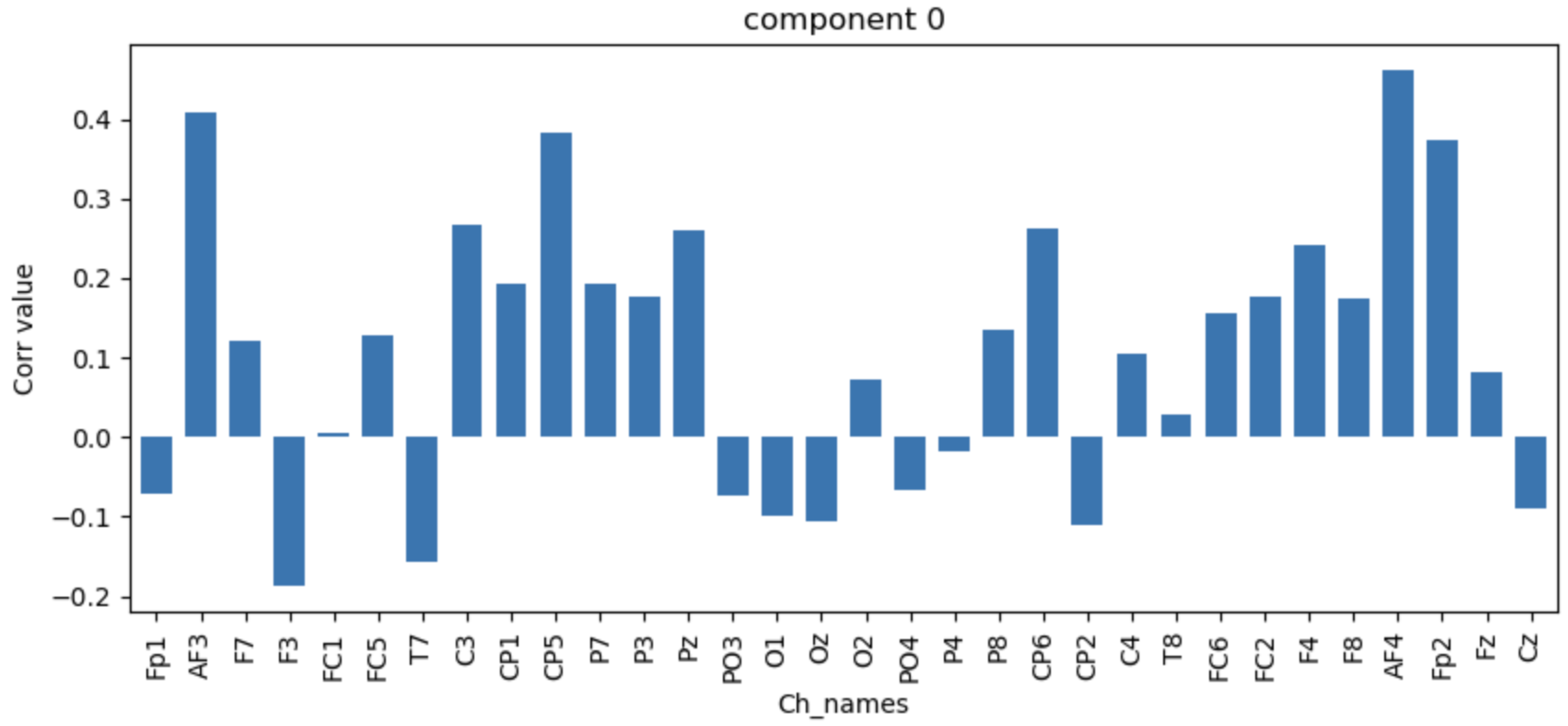
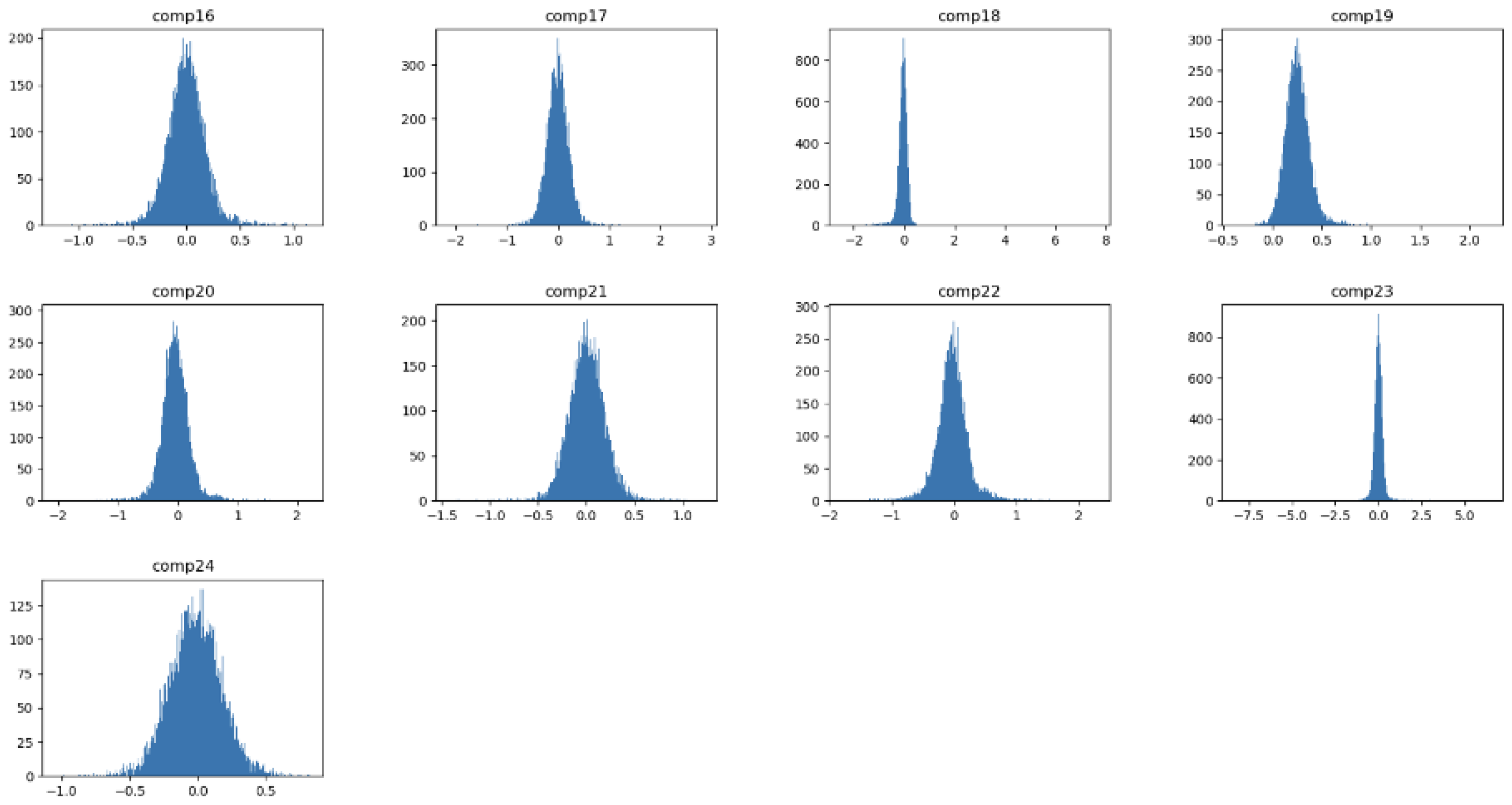
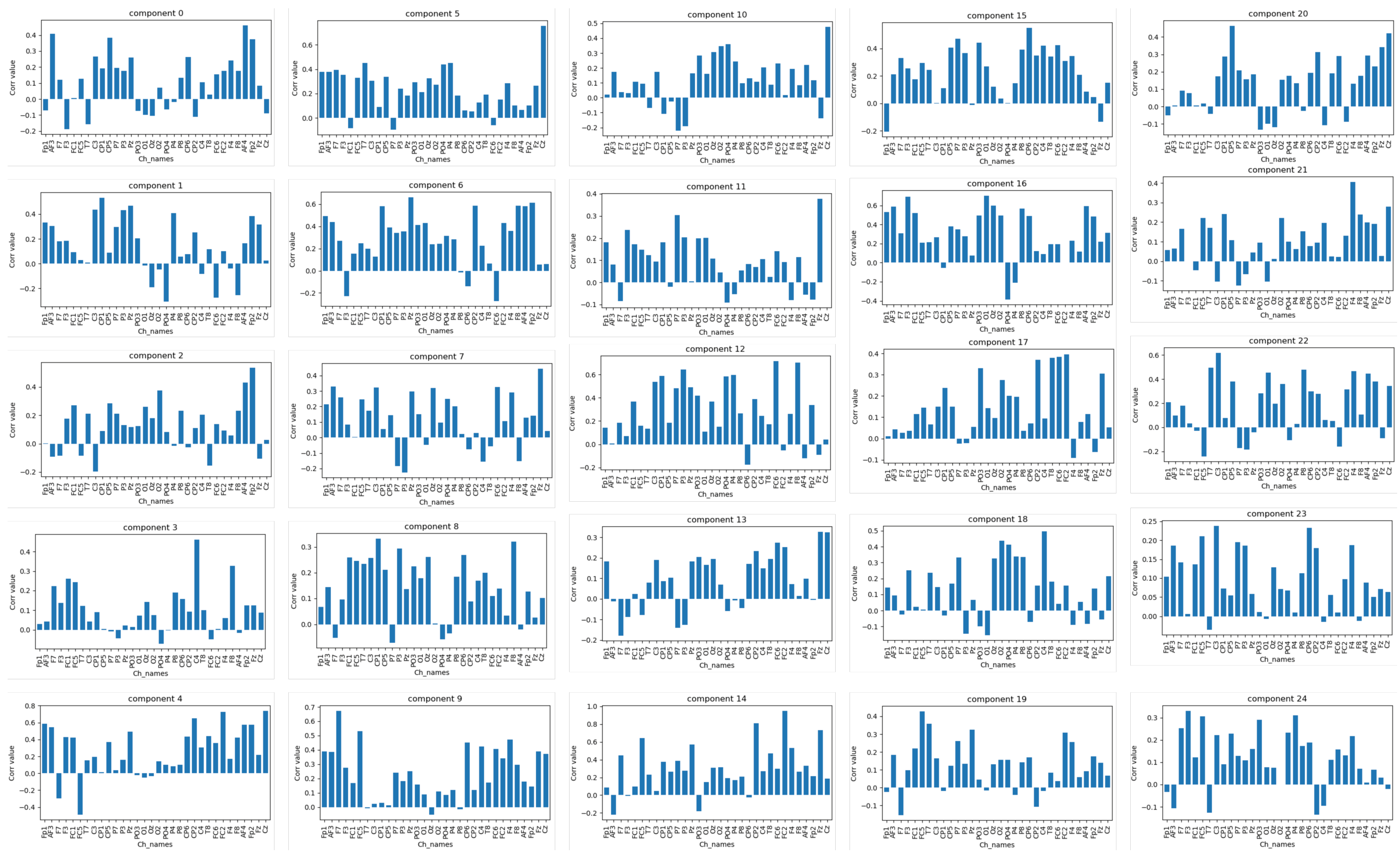
4.3. Interpreting and Visualising the Latent Space

This section describes the results obtained from interpreting the disentangled representation of CNN-VAE via visual plausibility and cluster analysis (Section 4.2). An empirical experiment was carried out using test data, with 10 samples chosen at random to assess the impact of each latent component in capturing the number of true generative factors in spatially preserving EEG topographic maps. Figure 7 depicts ten images of test data and reconstructed images with active latent space components 0 and 1, with visual plausibility results clearly indicating that each component is learning two to three patterns from those EEG topographic maps. To validate these findings, k-means clustering with the silhouette visualiser is used to demonstrate the contribution of each latent component to capturing the patterns in EEG topographic maps, which provides the exact number of generated patterns from each active component. The results show that each component in the latent space is responsible for generating a minimum of two patterns in the EEG topographic maps shown in Figure 8.
Finally, the reconstructed signal generated when setting up only one latent active component is transformed into EEG signals. In addition, 25 plots are generated to show the correlation values for each latent component grouped with all channels, shown in Figure A1 and Figure A2. Similarly, 32 plots for the correlation value for each channel aggregated with all components are generated; however, because of space constraints, only the top 25 plots for each channel are given in Appendix A, Figure A3. To make the decision of CNN-VAE easier to understand, the critical analysis was performed by activating only one latent component at a time. The resultant reconstruction EEG topo maps with each active latent component are coloured blue and yellow, where blue indicates it has some value that indicates the particular region of the brain in the topographic map is captured, and yellow represents an image filled with zeros. With latent component 0, the findings show that channel ‘FP1’ has a negative correlation while channel ‘AF4’ has a positive correlation with the original data, as shown in Figure 9. According to these findings, shown in the second row of Figure 7, and referencing with the 10–20 system of electrode placement used to describe the location of scalp electrodes in Figure 10, it is clearly indicated that component 0 of the latent space is less significant for acquiring left and right frontal pole in EEG topo maps.

5. Discussion

The results showed that when a CNN-VAE is trained with topographic maps of shape ( 40 , 40 ) comprising 1600 overall values produced from 32 electrode values, the size of the maps can be reduced by up to 99 % without losing salient information. In other words, each person-specific VAE may learn a latent space of up to 25 means and 25 standard deviations from a tensor of 1600 values without losing meaning, as measured by SSIM, MSE, MAE, and MAPE, between the original and reconstructed tensors.
The interpretation of CNN-VAE disentangled representation using visual plausibility and clustering analysis clearly shows that each component learns two to three patterns from those EEG topographic maps. These findings support the initial hypothesis, indicating that if CNN-VAE is trained with spatially preserved EEG topographic maps, it offers equivalent SNR and a stronger positive correlation between the architecture’s input and output EEG signal. Furthermore, the interpretation and visualisation of the learnt latent space representation aid in understanding the model’s choice.
The proposed pipeline for transforming EEG signals into a spatially preserved EEG topographic map, reconstructing EEG signals using CNN-VAE, and understanding the importance of each component in the latent space, as designed in Figure 2, has various advantages. To begin, convert the EEG signal into topographic maps that show the spatial distribution of the brain’s electrical activity. This study used DEAP data to train our model because it contains multi-channel EEG recordings with a large number of participants and tasks with 32 channels. This pipeline may easily be applied with various numbers of electrodes and can generate topographic maps of any size with other emotion datasets such as SEED and DREAMER. Since our pipeline produces topographic maps of 40 × 40 with 32 channels, it can also produce maps of the same size with a larger number of electrodes. Secondly, training CNN-VAE with EEG topographic maps yields latent space, which is a set of prominent high-level features with a lower dimension. This bottom dimension provides useful and salient EEG data representations that can be used to generate synthetic EEG topographic head maps for data augmentation and employability in a variety of classification tasks. Third, interpreting their latent space allows us to create useful visualisations that aid in the analysis of outcomes obtained in training a CNN-VAE with EEG signals. Interpreting the learned latent space helps us to understand the decisions of CNN-VAE and find the artefactual component in the CNN-VAE of latent space. Therefore, this method can be used for any kind of anomaly detection task. Since our suggested pipeline supports disentangled representation interpretation, it enables us to construct the required region of the image by manually setting up the latent space component. As a result, users can generate various images based on a single input image. The findings obtained from this proposed pipeline can be used to gain the trust of stakeholders by demonstrating the visual plausibility of each latent component in capturing the generative components in EEG topographic maps.
Aside from the implications, our suggested pipeline has some constraints because human brains are complex nonlinear systems generating nonstationary nonlinear signals [10]. Therefore, generating factors from each component vary from subject to subject, as do the number of electrodes and shape of the topographic maps employed. This pipeline requires human intervention to analyse and interpret its latent space. In future work, the interpretation of latent space must be performed automatically without human intervention to analyse the data from all participants with varied numbers of channels and topographic map sizes.

6. Conclusions

Researchers have designed and implemented different methods for interpreting the latent space of VAE. Most of the methods are used to improve the accuracy of classification tasks in a wide range of applications such as face recognition, video prediction, and anomaly detection. In most of the studies, its latent space interpretation is used to detect only the OOD latent variable for cluster analysis. However, understanding the decision of VAE requires investigating the significance of each latent component in the model’s decision. Therefore, interpreting its latent space via visual plausibility and clustering remains inadequate. The purpose of this study was to address this research challenge. An experiment has been conducted using an existing EEG dataset (DEAP) to understand the importance of each latent component of person-specific VAE. A CNN-VAE decoder network was trained with alternately one active latent component and the remaining components were set to zero because the mean value is close to zero in the distribution learnt from each latent component. Reconstructed EEG images generated from each latent active component were used as an input to k-means clustering to understand the number of generating factors learnt from each component. In addition, average and channel-wise correlation values with each component were computed to understand which component was responsible for activating which part of the brain. The results show that each component contributes differently to capturing and generating aspects in topographic maps, which are visualised using clustering techniques. Hence, this pipeline can be used to generate any size of EEG topo maps with any number of channels. This proposed pipeline is tested on only one participant’s data. However, generating factors from each component may vary from participant to participant, as well as the number of electrodes and shape of the topographic maps employed. Future studies will include the automatic interpretation of the CNN-VAE latent space without human intervention to support the EEG data from all participants with varied numbers of channels and topographic map sizes. In addition, performing the interpretation of its latent representation reduces the artefacts by setting the specific component of the CNN-VAE latent space. Furthermore, a complete pipeline will be designed, which will automatically reduce the number of artefacts in EEG signals.

Author Contributions

Conceptualisation, Formal analysis, Investigation, Methodology, Project administration, Resources, Software, T.A. and L.L.; Supervision, L.L.; Validation, T.A. and L.L.; Visualization, T.A.; Writing—original draft, T.A.; Writing—review & editing, T.A. and L.L. All authors have read and agreed to the published version of the manuscript.

Funding

Technological University Dublin, Ireland, under grant PB04433.

Data Availability Statement

DEAP dataset: a dataset for emotion analysis using EEG, physiological, and video signals https://www.eecs.qmul.ac.uk/mmv/datasets/deap/ (accessed on 10 January 2021).

Conflicts of Interest

The authors declare no conflict of interest.

Abbreviations

The following abbreviations are used in this manuscript:
EEGElectroencephalography
AEAutoencoder
VAEVaraiational autoencoder
CNN-VAEConvolutional variational autoencoder
SNRSignal-to-noise ratio
XAIExplainable artificial intelligence
SVHNStreet-view house number
ARAttribute-regularized
GANGenerative adversarial network
DLSDisentangling latent space
GMMGaussian mixture model
MMDMaximum mean discrepancy
SSIMStructural similarity
MSEMean squared error
MAEMean absolute error
MAPEMean absolute percentage error

Appendix A

Figure A1. Distribution of all latent spaces when one latent component is active at a time.
Information 14 00489 g0a1aInformation 14 00489 g0a1b
Figure A2. Correlation values between the original and reconstructed signal generated from each latent active component grouped with all channels.
Information 14 00489 g0a2
Figure A3. Correlation values between the original and reconstructed signal for each channel grouped with all latent components.
Information 14 00489 g0a3

References

  1. Binnie, C.; Prior, P. Electroencephalography. J. Neurol. Neurosurg. Psychiatry 1994, 57, 1308–1319. [Google Scholar] [CrossRef]
  2. Khare, S.K.; March, S.; Barua, P.D.; Gadre, V.M.; Acharya, U.R. Application of data fusion for automated detection of children with developmental and mental disorders: A systematic review of the last decade. Inf. Fusion 2023, 99, 101898. [Google Scholar] [CrossRef]
  3. Hooi, L.S.; Nisar, H.; Voon, Y.V. Comparison of motion field of EEG topo-maps for tracking brain activation. In Proceedings of the 2016 IEEE EMBS Conference on Biomedical Engineering and Sciences (IECBES), Kuala Lumpur, Malaysia, 4–8 December 2016; pp. 251–256. [Google Scholar]
  4. Anderson, E.W.; Preston, G.A.; Silva, C.T. Using python for signal processing and visualization. Comput. Sci. Eng. 2010, 12, 90–95. [Google Scholar] [CrossRef]
  5. Ahmed, T.; Longo, L. Examining the Size of the Latent Space of Convolutional Variational Autoencoders Trained With Spectral Topographic Maps of EEG Frequency Bands. IEEE Access 2022, 10, 107575–107586. [Google Scholar] [CrossRef]
  6. Chikkankod, A.V.; Longo, L. On the dimensionality and utility of convolutional Autoencoder’s latent space trained with topology-preserving spectral EEG head-maps. Mach. Learn. Knowl. Extr. 2022, 4, 1042–1064. [Google Scholar] [CrossRef]
  7. Anwar, A.M.; Eldeib, A.M. EEG signal classification using convolutional neural networks on combined spatial and temporal dimensions for BCI systems. In Proceedings of the 2020 42nd Annual International Conference of the IEEE Engineering in Medicine & Biology Society (EMBC), Montreal, QC, Canada, 20–24 July 2020; pp. 434–437. [Google Scholar]
  8. Taherisadr, M.; Joneidi, M.; Rahnavard, N. EEG signal dimensionality reduction and classification using tensor decomposition and deep convolutional neural networks. In Proceedings of the 2019 IEEE 29th International Workshop on Machine Learning for Signal Processing (MLSP), Pittsburgh, PA, USA, 13–16 October 2019; pp. 1–6. [Google Scholar]
  9. Miladinović, A.; Ajčević, M.; Jarmolowska, J.; Marusic, U.; Colussi, M.; Silveri, G.; Battaglini, P.P.; Accardo, A. Effect of power feature covariance shift on BCI spatial-filtering techniques: A comparative study. Comput. Methods Programs Biomed. 2021, 198, 105808. [Google Scholar] [CrossRef] [PubMed]
  10. Klonowski, W. Everything you wanted to ask about EEG but were afraid to get the right answer. Nonlinear Biomed. Phys. 2009, 3, 1–5. [Google Scholar] [CrossRef]
  11. Lotte, F.; Congedo, M.; Lécuyer, A.; Lamarche, F.; Arnaldi, B. A review of classification algorithms for EEG-based brain–computer interfaces. J. Neural Eng. 2007, 4, R1. [Google Scholar] [CrossRef]
  12. Bao, G.; Yan, B.; Tong, L.; Shu, J.; Wang, L.; Yang, K.; Zeng, Y. Data augmentation for EEG-based emotion recognition using generative adversarial networks. Front. Comput. Neurosci. 2021, 15, 723843. [Google Scholar] [CrossRef]
  13. Bengio, Y.; Courville, A.; Vincent, P. Representation learning: A review and new perspectives. IEEE Trans. Pattern Anal. Mach. Intell. 2013, 35, 1798–1828. [Google Scholar] [CrossRef]
  14. Vincent, P.; Larochelle, H.; Bengio, Y.; Manzagol, P.A. Extracting and composing robust features with denoising autoencoders. In Proceedings of the 25th International Conference on Machine Learning, Helsinki, Finland, 5–9 July 2008; pp. 1096–1103. [Google Scholar]
  15. Bornschein, J.; Bengio, Y. Reweighted wake-sleep. arXiv 2014, arXiv:1406.2751. [Google Scholar]
  16. Abdelfattah, S.M.; Abdelrahman, G.M.; Wang, M. Augmenting the size of EEG datasets using generative adversarial networks. In Proceedings of the 2018 International Joint Conference on Neural Networks (IJCNN), Rio de Janeiro, Brazil, 8–13 July 2018; pp. 1–6. [Google Scholar]
  17. Hwaidi, J.F.; Chen, T.M. A Noise Removal Approach from EEG Recordings Based on Variational Autoencoders. In Proceedings of the 2021 13th International Conference on Computer and Automation Engineering (ICCAE), Melbourne, Australia, 20–22 March 2021; pp. 19–23. [Google Scholar]
  18. Li, K.; Wang, J.; Li, S.; Yu, H.; Zhu, L.; Liu, J.; Wu, L. Feature Extraction and Identification of Alzheimer’s Disease based on Latent Factor of Multi-Channel EEG. IEEE Trans. Neural Syst. Rehabil. Eng. 2021, 29, 1557–1567. [Google Scholar] [CrossRef]
  19. Kingma, D.P.; Welling, M. Auto-encoding variational bayes. arXiv 2013, arXiv:1312.6114. [Google Scholar]
  20. Li, X.; Zhao, Z.; Song, D.; Zhang, Y.; Pan, J.; Wu, L.; Huo, J.; Niu, C.; Wang, D. Latent factor decoding of multi-channel EEG for emotion recognition through autoencoder-like neural networks. Front. Neurosci. 2020, 14, 87. [Google Scholar] [CrossRef]
  21. Zheng, Z.; Sun, L. Disentangling latent space for vae by label relevant/irrelevant dimensions. In Proceedings of the IEEE/CVF Conference on Computer Vision and Pattern Recognition, Long Beach, CA, USA, 15–20 June 2019; pp. 12192–12201. [Google Scholar]
  22. Peng, X.; Yu, X.; Sohn, K.; Metaxas, D.N.; Chandraker, M. Reconstruction-based disentanglement for pose-invariant face recognition. In Proceedings of the IEEE International Conference on Computer Vision, Venice, Italy, 22–29 October 2017; pp. 1623–1632. [Google Scholar]
  23. Hsieh, J.T.; Liu, B.; Huang, D.A.; Fei-Fei, L.F.; Niebles, J.C. Learning to decompose and disentangle representations for video prediction. Adv. Neural Inf. Process. Syst. 2018, 31. [Google Scholar] [CrossRef]
  24. Wang, S.; Chen, T.; Chen, S.; Nepal, S.; Rudolph, C.; Grobler, M. Oiad: One-for-all image anomaly detection with disentanglement learning. In Proceedings of the 2020 International Joint Conference on Neural Networks (IJCNN), Glasgow, UK, 19–24 July 2020; pp. 1–8. [Google Scholar]
  25. Siddharth, N.; Paige, B.; Desmaison, A.; Van de Meent, J.W.; Wood, F.; Goodman, N.D.; Kohli, P.; Torr, P.H. Inducing interpretable representations with variational autoencoders. arXiv 2016, arXiv:1611.07492. [Google Scholar]
  26. Ramakrishna, S.; Rahiminasab, Z.; Karsai, G.; Easwaran, A.; Dubey, A. Efficient out-of-distribution detection using latent space of β-vae for cyber-physical systems. ACM Trans. Cyber-Phys. Syst. (TCPS) 2022, 6, 1–34. [Google Scholar] [CrossRef]
  27. Mathieu, E.; Rainforth, T.; Siddharth, N.; Teh, Y.W. Disentangling disentanglement in variational autoencoders. In Proceedings of the International Conference on Machine Learning, PMLR, Long Beach, CA, USA, 9–15 June 2019; pp. 4402–4412. [Google Scholar]
  28. Spinner, T.; Körner, J.; Görtler, J.; Deussen, O. Towards an interpretable latent space: An intuitive comparison of autoencoders with variational autoencoders. In Proceedings of the IEEE VIS, Berlin, Germany, 27 October 2018. [Google Scholar]
  29. Bryan-Kinns, N.; Banar, B.; Ford, C.; Reed, C.; Zhang, Y.; Colton, S.; Armitage, J. Exploring xai for the arts: Explaining latent space in generative music. arXiv 2022, arXiv:2308.05496 2022. [Google Scholar]
  30. Pati, A.; Lerch, A. Attribute-based regularization of latent spaces for variational auto-encoders. Neural Comput. Appl. 2021, 33, 4429–4444. [Google Scholar] [CrossRef]
  31. Dinari, O.; Freifeld, O. Variational-and metric-based deep latent space for out-of-distribution detection. In Proceedings of the 38th Conference on Uncertainty in Artificial Intelligence, Eindhoven, The Netherlands, 1–5 August 2022. [Google Scholar]
  32. Ding, F.; Yang, Y.; Luo, F. Clustering by directly disentangling latent space. In Proceedings of the 2022 IEEE International Conference on Image Processing (ICIP), Bordeaux, France, 16–19 October 2022; pp. 341–345. [Google Scholar]
  33. Mukherjee, S.; Asnani, H.; Lin, E.; Kannan, S. Clustergan: Latent space clustering in generative adversarial networks. In Proceedings of the AAAI Conference on Artificial Intelligence, Honolulu, HI, USA, 27 January–1 February 2019; Volume 33, pp. 4610–4617. [Google Scholar]
  34. Prasad, V.; Das, D.; Bhowmick, B. Variational clustering: Leveraging variational autoencoders for image clustering. In Proceedings of the 2020 International Joint Conference on Neural Networks (IJCNN), Glasgow, UK, 19 July 2020; pp. 1–10. [Google Scholar] [CrossRef]
  35. Koelstra, S.; Muhl, C.; Soleymani, M.; Lee, J.S.; Yazdani, A.; Ebrahimi, T.; Pun, T.; Nijholt, A.; Patras, I. Deap: A database for emotion analysis; using physiological signals. IEEE Trans. Affect. Comput. 2011, 3, 18–31. [Google Scholar] [CrossRef]
  36. Hwaidi, J.F.; Chen, T.M. A Novel KOSFS Feature Selection Algorithm for EEG Signals. In Proceedings of the IEEE EUROCON 2021—19th International Conference on Smart Technologies, Lviv, Ukraine, 6–8 July 2021; pp. 265–268. [Google Scholar]
  37. Kingma, D.P.; Welling, M. Auto-encoding variational bayes in 2nd International Conference on Learning Representations. In Proceedings of the ICLR 2014-Conference Track Proceedings, Banff, AB, Canada, 14–16 April 2014. [Google Scholar]
  38. Gretton, A.; Borgwardt, K.; Rasch, M.J.; Scholkopf, B.; Smola, A.J. A kernel method for the two-sample problem. arXiv 2008, arXiv:0805.2368. [Google Scholar]
  39. Sara, U.; Akter, M.; Uddin, M.S. Image quality assessment through FSIM, SSIM, MSE and PSNR—A comparative study. J. Comput. Commun. 2019, 7, 8–18. [Google Scholar] [CrossRef]
  40. Schneider, P.; Xhafa, F. Chapter 3—Anomaly detection: Concepts and methods. In Anomaly Detection and Complex Event Processing over IoT Data Streams; Elsevier: Amsterdam, The Netherlands, 2022; pp. 49–66. [Google Scholar]
  41. Asuero, A.G.; Sayago, A.; González, A. The correlation coefficient: An overview. Crit. Rev. Anal. Chem. 2006, 36, 41–59. [Google Scholar] [CrossRef]
  42. Hanrahan, C. Noise Reduction in Eeg Signals Using Convolutional Autoencoding Techniques. Master’s Thesis, Technological University Dublin, Dublin, Ireland, 1 September 2019. [Google Scholar]
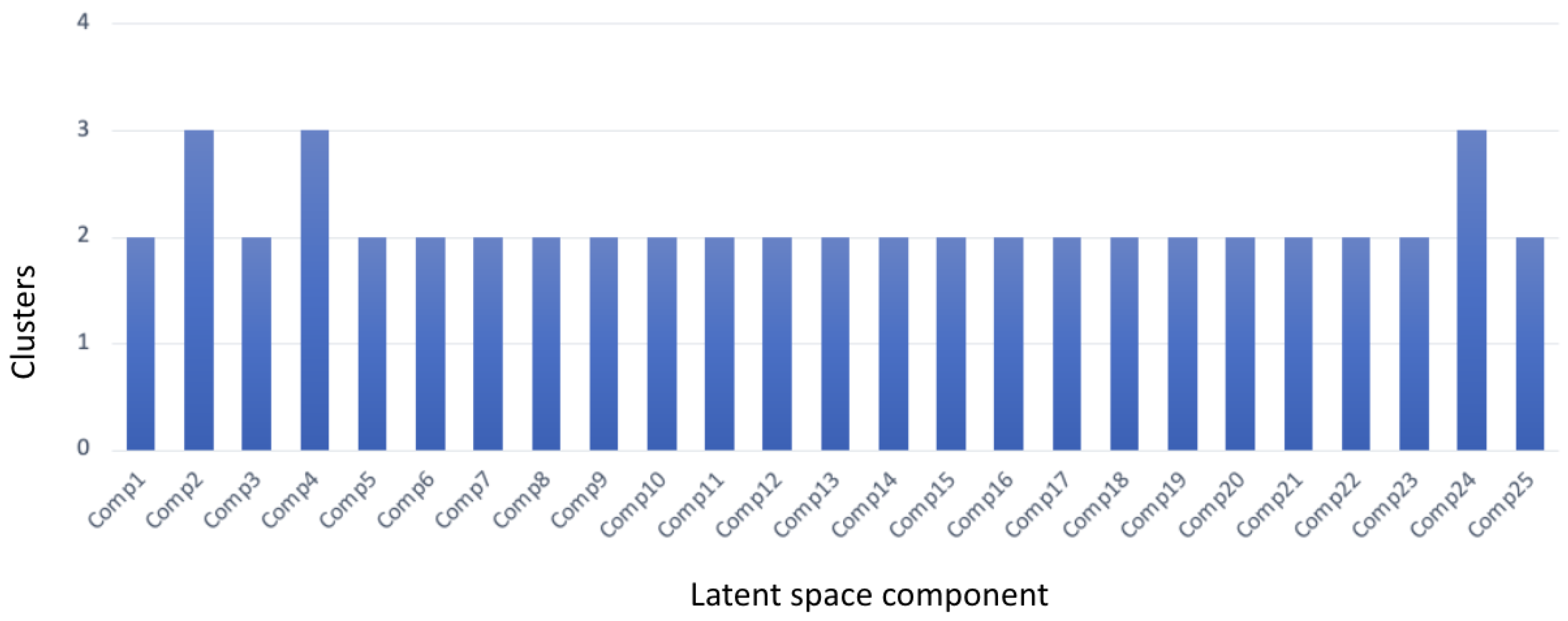
Figure 1. The structure of a variational autoencoder (VAE) leverages convolutional methods on input data that maps these data into the parameters of a probability distribution, such as the mean and the variance of a Gaussian distribution.
Information 14 00489 g001
Figure 2. A pipeline for spatially preserving EEG topographic map generation and interpreting the latent space of CNN-VAE via clustering and visual plausibility. (A) The DEAP dataset was used to build a CNN-VAE from EEG signals. (B) EEG topographic head maps of size 40 × 40 generation. (C) A CNN-VAE model is learnt for a variable by variable interpretation of the latent space. (D) Clustering for visualising the learnt pattern from each active latent component. (E) Reconstruction of the signals from 32 electrode coordinate values of EEG topographic maps. (F) Evaluation of the model for reconstructed topographic maps as well as the signal.
Information 14 00489 g002
Figure 3. An example of average Euclidian distance computed from channel index of topographic maps ranging in size from 26 to 64.
Information 14 00489 g003
Figure 4. Distribution of the four latent spaces when one latent component is active at a time.
Information 14 00489 g004
Figure 5. Signal from the T7 and P7 channels, as well as their correlation values with the original data’s channel values.
Information 14 00489 g005
Figure 6. SNR for each channel of the original and reconstructed test data.
Information 14 00489 g006
Figure 7. Randomly selected 10 samples of actual and reconstructed topo maps with active components 0 and 1 of the latent space.
Information 14 00489 g007
Figure 8. Cluster analysis on reconstructed test EEG topo maps generated from each latent space active component.
Information 14 00489 g008
Figure 9. Correlation values computed between original and reconstructed signals generated with latent space component 0.
Information 14 00489 g009
Figure 10. 10–20 system of electrode placement in EEG topographic maps of size 40 × 40.
Information 14 00489 g010
Table 1. An example of the SSIM, MSE, MAE, MAPE, SNR, average correlation, and a number of clusters generated after interpreting the latent space of a one-person-specific convolutional variational autoencoder (CNN-VAE) on testing data.
CompSSIMMSEMAEMAPESNRAvgCorrCluster
C 1-251.00000.0000001030.000190.000420.366978830.994
C10.99690.00003750.002960.004840.1080.1072
C20.99700.00003690.002920.004780.0920.1343
C30.99690.00003740.002960.004840.1070.1192
C40.99690.00003760.002960.004851.2410.0953
C50.99730.00003090.002900.004740.1140.2672
C60.99710.00003410.002860.004670.1170.2362
C70.99700.00003530.002870.004700.0960.2832
C80.99690.00003730.002940.004810.1530.1182
C90.99690.00003740.002950.004820.1120.142
C100.99710.00003520.002870.004700.0990.2312
C110.99690.00003730.002960.004830.1030.1162
C120.99690.00003760.002960.004840.0880.092
C130.99710.00003510.002830.004630.110.2782
C140.99690.00003770.002970.004860.0580.0892
C150.99740.00002950.002830.004630.1150.2942
C160.99700.0000360.002850.004670.10.2232
C170.99700.00003470.002800.004590.0990.3022
C180.99690.00003740.002960.004850.0960.1362
C190.99690.00003740.002950.004830.1070.1252
C200.99690.00003740.002950.004830.3040.1232
C210.99700.00003680.002940.004800.1040.1262
C220.99700.00003740.002960.004840.1150.0992
C230.99700.00003580.002910.004750.0850.1762
C240.99690.00003790.002980.004870.1030.0923
C250.99690.00003770.002970.004850.1330.1122
Disclaimer/Publisher’s Note: The statements, opinions and data contained in all publications are solely those of the individual author(s) and contributor(s) and not of MDPI and/or the editor(s). MDPI and/or the editor(s) disclaim responsibility for any injury to people or property resulting from any ideas, methods, instructions or products referred to in the content.

