Time-Series Neural Network: A High-Accuracy Time-Series Forecasting Method Based on Kernel Filter and Time Attention

Abstract

This research introduces a novel high-accuracy time-series forecasting method, namely the Time Neural Network (TNN), which is based on a kernel filter and time attention mechanism. Taking into account the complex characteristics of time-series data, such as non-linearity, high dimensionality, and long-term dependence, the TNN model is designed and implemented. The key innovations of the TNN model lie in the incorporation of the time attention mechanism and kernel filter, allowing the model to allocate different weights to features at each time point, and extract high-level features from the time-series data, thereby improving the model’s predictive accuracy. Additionally, an adaptive weight generator is integrated into the model, enabling the model to automatically adjust weights based on input features. Mainstream time-series forecasting models such as Recurrent Neural Networks (RNNs) and Long Short-Term Memory Networks (LSTM) are employed as baseline models and comprehensive comparative experiments are conducted. The results indicate that the TNN model significantly outperforms the baseline models in both long-term and short-term prediction tasks. Specifically, the RMSE, MAE, and $R^2$ reach 0.05, 0.23, and 0.95, respectively. Remarkably, even for complex time-series data that contain a large amount of noise, the TNN model still maintains a high prediction accuracy.

1. Introduction

With the rapid development of global financial markets, the stock market has increasingly become a significant choice for investors. In the stock market, the accuracy of stock price prediction directly influences investors’ decisions and is crucial for the health and stability of economic activities. However, stock price prediction poses a formidable challenge. Stock prices are influenced by numerous factors, including but not limited to macroeconomic conditions, company performance reports, market sentiment, and even global political dynamics. The interweaving of these factors causes stock prices to exhibit a high degree of uncertainty and non-linearity, which adds significant difficulty to forecasting.

In recent years, deep learning has made considerable contributions in fields such as agriculture [1,2], healthcare [3,4], energy usage [5], and finance [6]. This development provides a new solution for the time series prediction problem. Neural network models have gradually been widely used in stock price prediction due to their advantages in processing non-linear data and capturing long-distance dependencies. Nevertheless, most existing prediction models based on neural networks often overlook a critical issue, the temporal attributes of stock prices and their importance. In reality, the impact of past price trends on future prices is not equal; recent price changes often have a more significant effect on future price predictions.

In recent decades, many researchers and practitioners have tried to predict stock prices using various methods, including time-series-based prediction methods [7,8], machine learning-based prediction methods [9,10], deep learning-based prediction methods [11,12,13,14], and so on. However, due to the characteristics of stock prices, such as non-linearity, high noise, and variability, it is often difficult to achieve the desired prediction results with these methods [15,16,17,18,19,20,21].

To address this problem, a time-series neural network method based on Kernel Filter and Time Attention is proposed in this paper, both of which are novel applications developed by the authors for achieving higher accuracy in stock price prediction. Firstly, the Kernel Filter is incorporated into the neural network model to effectively extract the features of time-series data, especially in handling data with noise. This is a novel application aiming to improve upon existing filtering techniques in neural networks. By applying Kernel Filter, it is possible to capture the underlying trends of stock prices more accurately and eliminate irrelevant noise interference, thereby enhancing the accuracy of predictions. Secondly, a novel Time Attention mechanism is designed that assigns higher weights to recent data, a unique approach developed to extend the capabilities of existing attention mechanisms in capturing the temporal characteristics of stock prices. The advantage of this approach is that it can more effectively capture the dynamics of recent prices, which often serves as a crucial factor in predicting future prices. With these two innovative designs, the proposed model considers the characteristics of time-series data, effectively extracts data features, and pays more attention to recent data, thereby achieving higher accuracy in stock price prediction.

In addition to introducing these innovative techniques, a series of carefully designed experiments was conducted to measure the model’s performance against established benchmarks in the field, such as RNN and LSTM. Our findings confirm that the TNN stands up exceptionally well when challenged with various forecasting tasks, making it particularly suitable for predicting stock prices. Notably, the model’s performance remains robust even when applied to noisy, complex time-series data. Detailed evaluations and comparisons are presented in the subsequent sections, reaffirming the model’s superior predictive power with noteworthy metrics.

In the future, there are plans to further optimize the model and verify it on more financial datasets, with the aim of further enhancing the model’s generalization ability and prediction accuracy.

2. Related Work

Times-series forecasting has continually served as a research hotspot in the field of finance, with its core premise being to decipher patterns from historical data to predict future price fluctuations. To tackle this issue, researchers have implemented a variety of machine learning methods, which include both traditional machine learning methods and deep learning techniques.

2.1. Traditional Machine Learning Methods

In early research endeavors, traditional machine learning methods were ubiquitously employed for stock price prediction. These methods encompassed Linear Regression (LR) [22], SVM [23], and Decision Trees [24], among others. Linear Regression, a fundamental prediction model, primarily extrapolates based on the linear relationship between inputs and outputs. Its basic form is as follows:

$$y=aX+b$$

(1)

where X denotes the input variables, y the output variables, and a and b the model parameters to be learned. However, as stock prices are influenced by a multitude of factors, the inherent laws are often non-linear. Consequently, the linear regression model struggles to capture this complexity.

Support Vector Machine, a common method for both classification and regression, operates by finding an optimal hyperplane to separate the data, thereby achieving the goal of prediction. For regression problems, the form of SVM is as follows:

$$f\left(X\right)=\langle w,\varphi \left(X\right)\rangle +b$$

(2)

where $\varphi \left(X\right)$ represents the feature mapping of input variables X, w and b are the model parameters to be learned, and $\langle w,\varphi \left(X\right)\rangle$ denotes the inner product of w and $\varphi \left(X\right)$. Although SVM can handle non-linear problems, its high computational complexity when applied to high-dimensional and large-scale datasets proves to be a substantial obstacle.

Traditional machine learning methods like SVM, Random Forests, and Decision Trees often encounter several limitations in the context of stock price prediction. SVMs [25], while effective for linearly separable problems, struggle with handling high dimensionality and require substantial tuning, including the choice of an appropriate kernel function for non-linear financial time-series data. Random Forests [26], although they offer an improvement over Decision Trees by ensemble learning, still suffer from high computational complexity and can underperform when dealing with highly noisy and volatile markets. Decision Trees, on the other hand, are simple to implement and interpret but are prone to overfitting, especially when grappling with the complex, noisy, and erratic nature of stock markets. These methods often require manual feature engineering and generally fail to capture the intricate, non-linear patterns and long-term dependencies that are inherent to financial time-series data.

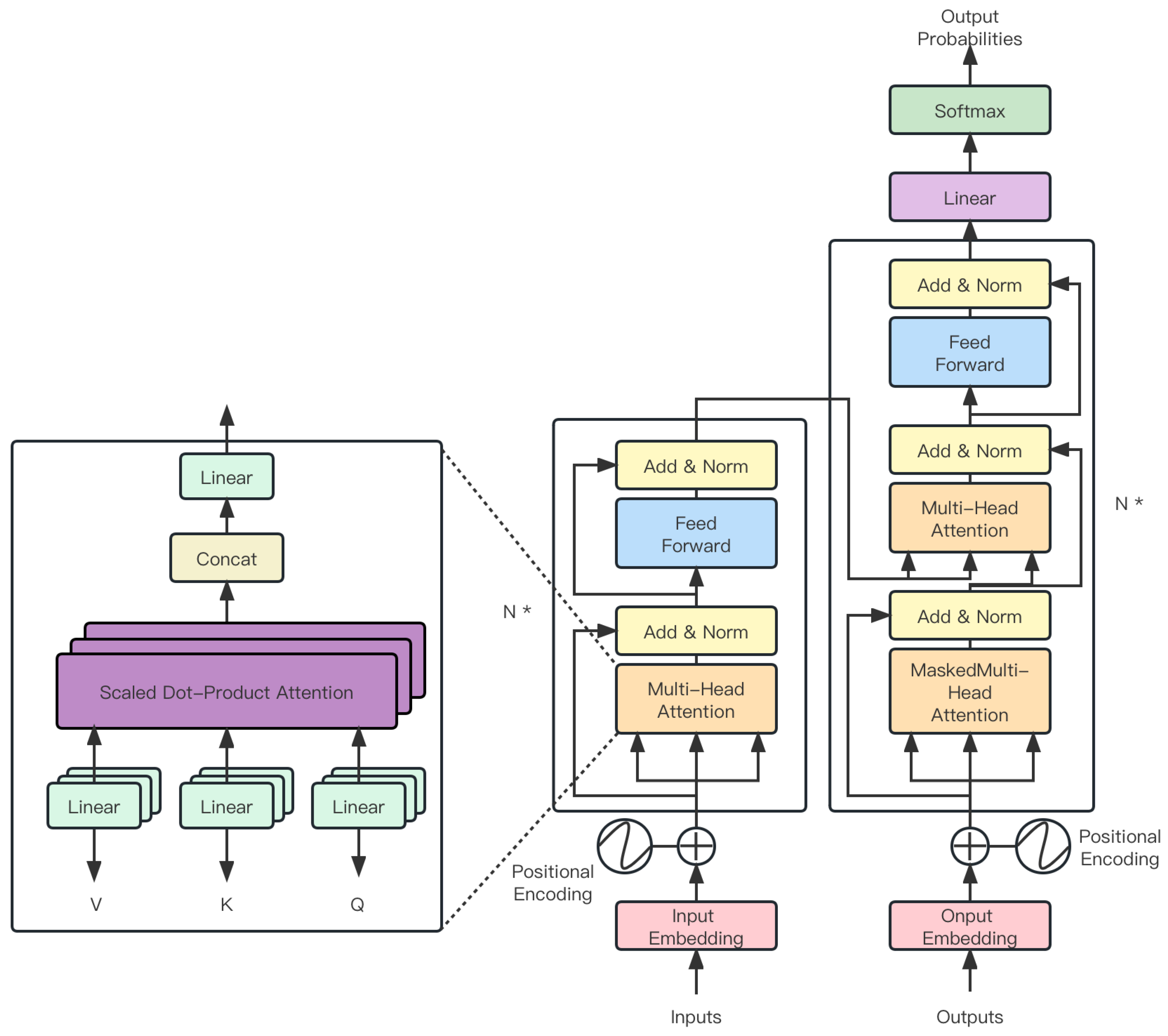
2.2. Deep Learning Methods

In recent years, deep learning methods, particularly RNN [27] and LSTM [28], have found extensive application in the field of stock price prediction. RNN, a neural network with memory function, is capable of capturing temporal relationships within sequence data. Its basic formula is as follows:

$$h_t=\sigma (W_{hh}{h}_{t-1}+W_{xh}{x}_t+b_h)$$

(3)

$$y_t=W_{hy}{h}_t+b_y$$

(4)

where $x_t$ is the input, $h_t$ the hidden state, $y_t$ the output, $\sigma$ the activation function, $W_{hh}$, $W_{xh}$, and $W_{hy}$ the weight parameters, and $b_h$ and $b_y$ the bias parameters. Although RNNs can handle sequence data, they suffer from vanishing and exploding gradients in long sequences, making it challenging to capture long-term dependencies.

LSTM, an improved RNN, introduces a gating mechanism to resolve the issue of long-term dependencies. The basic formula of LSTM is as follows:

$$\begin{array}{cc}\hfill f_t& =\sigma (W_f[h_{t-1},x_t]+b_f)\hfill \\ \hfill i_t& =\sigma (W_i[h_{t-1},x_t]+b_i)\hfill \\ \hfill {\tilde{C}}_t& =tanh(W_C[h_{t-1},x_t]+b_C)\hfill \\ \hfill C_t& =f_t\ast C_{t-1}+i_t\ast {\tilde{C}}_t\hfill \\ \hfill o_t& =\sigma (W_o[h_{t-1},x_t]+b_o)\hfill \\ \hfill h_t& =o_t\ast tanh\left(C_t\right)\hfill \end{array}$$

(5)

where $f_t$, $i_t$, and $o_t$ are the forget gate, input gate, and output gate, respectively, $C_t$ is the cell state, $\sigma$ is the sigmoid function, tanh is the tanh function, ∗ represents element-wise multiplication, and $[h_{t-1},x_t]$ denotes the concatenation of $h_{t-1}$ and $x_t$. While LSTM exhibits commendable performance in certain tasks, it also encounters several issues, such as possessing numerous parameters, high computational complexity, and difficulty in dealing with discontinuous and irregular time-series data.

While RNN and LSTMs have been popular for time-series forecasting, including stock price prediction, they also come with their own sets of challenges. RNNs [29,30], for example, are prone to issues like vanishing and exploding gradients when handling long sequences, making them less effective for capturing long-term dependencies in stock price data. LSTMs, designed to mitigate some of these issues, are computationally expensive and still might require substantial parameter tuning for optimal performance [31,32]. Additionally, both RNNs and LSTMs can be sensitive to hyperparameter settings, making them less robust when applied to the highly volatile and noisy nature of stock markets.

In summary, both traditional machine learning methods and deep learning techniques come with their respective advantages and drawbacks. In this work, a new time-series neural network is proposed, integrating Kernel Filter and Time Attention mechanisms, aiming to resolve the issues present in the aforementioned methods when applied to stock price prediction.

3. Materials and Methods

3.1. Dataset Collection

In this research, a decade of stock data from the S&P 500 index was selected as the experimental dataset. The 10-year span was chosen to offer a comprehensive yet computationally feasible dataset for modeling. This timeframe incorporates various market conditions, including both bull and bear phases, high- and low-volatility periods, and multiple economic cycles. While a decade may not capture the full complexity and cyclical nature of stock markets, it provides a rich set of data that allows for robust modeling and prediction. Additionally, using a decade-long data sample enables the evaluation of the model’s performance across a variety of scenarios, thereby enhancing the generalizability of the study’s findings. It should be noted that although the 10-year dataset is comprehensive in some respects, the scope of this research could be further expanded in future studies by incorporating a larger and more diverse set of data points.

The S&P 500 index, a stock market index released by the Standard & Poor’s Financial Services company, encompasses the largest 500 listed companies in the U.S. market. The choice of the S&P 500 was based on two reasons. First, the S&P 500 index covers a broad range of U.S. stock market sectors, with constituent stocks originating from various industries such as technology, healthcare, finance, consumer, and industry. This extensive coverage implies that the collected dataset is representative and can reflect the overall status of the U.S. stock market. Second, the S&P 500 has a large volume of historical data, spanning a long timeframe. Nearly a decade of stock data was collected, providing ample training samples beneficial for the machine learning model’s learning and generalization.

To obtain these data, Python and the BeautifulSoup framework were utilized to develop a web scraper. Python, with its concise syntax, extensive library functions, and wide community support, is extensively used in the field of data science. BeautifulSoup is a Python library that facilitates parsing HTML code from webpages, extracting the required information. In the specific implementation process, the source of data was identified as the Yahoo Finance website. Yahoo Finance offers abundant historical stock data and permits users to download data in CSV format. A web scraper was developed to automatically download historical data of the S&P 500 constituent stocks. In the scraper, the principle of “respecting the Robots protocol” was adhered to, setting a reasonable access interval to avoid imposing unnecessary pressure on the server. The collected data include information such as the opening price, highest price, lowest price, closing price, and trading volume of each trading day. The data span from 2013 to 2023, a total of ten years. This approach to data collection not only provided abundant, high-quality stock data but also ensured the data’s timeliness and completeness.

3.2. Dataset Preprocessing

3.2.1. Outlier Identification and Treatment

The first step was outlier identification and treatment. Outliers could potentially have a detrimental effect on model learning, leading to inaccurate prediction results. Hence, identifying and handling these outliers is crucial for ensuring model performance. In this work, the 3$\sigma$ rule was initially applied as a general guideline for outlier identification, under the assumption of a normal distribution. Given the non-stationary nature of the data, as well as the presence of fat tails and skewness, this method serves as a heuristic rather than an absolute criterion for outlier detection. Under the assumption of normal distribution, any value that diverges from the mean by more than three times the standard deviation is considered an outlier. The specific formula is as follows:

$$\begin{array}{cc}\hfill & \mu =\frac{1}{N}\sum _{i=1}^N{x}_i\hfill \\ \hfill & \sigma =\sqrt{\frac{1}{N}\sum _{i=1}^N{(x_i-\mu )}^2}\hfill \\ \hfill & if|x_i-\mu |>3\sigma ,x_{i}isanoutlier\hfill \end{array}$$

(6)

Here, N represents the number of samples, $x_i$ represents the value of a single sample, and $\mu$ and $\sigma$ are the sample mean and standard deviation, respectively. After identifying potential outliers, the median of the corresponding feature was used for replacement. The median is robust to outlier perturbation and thus serves as a reliable measure for this purpose. In our dataset, the actual number of outliers identified and replaced was 1.38% of the total number of data points.

3.2.2. Missing Value Treatment

In the collected raw data, there might be missing values. Ignoring or simply deleting these missing values could result in information loss, subsequently affecting the model’s learning performance. Therefore, these missing values needed treatment. In this study, interpolation was employed to fill in missing values. Specifically, linear interpolation was used, assuming that the data could be linearly expressed at the missing point. The formula is as follows:

$$x_{miss}=x_{before}+\frac{x_{after}-x_{before}}{2}$$

(7)

Here, $x_{miss}$ represents the missing value, while $x_{before}$ and $x_{after}$ are the observed values before and after the missing value, respectively.

3.2.3. Normalization

After treating outliers, we also addressed missing values in the data. In our dataset, a total of 218 missing values were observed across “Open”, “High”, “Low”, “Close”, and “Vol” prices. These missing values were handled using normalization. Given that the scales and value ranges of different features may vary, inputting them directly into the model might impact the model’s learning performance. Through normalization, the value range of all features could be adjusted to a unified interval, avoiding the model’s over-dependence on features with large values. Min-max normalization, also known as linear normalization, was adopted. The formula is as follows:

$$x_{norm}=\frac{x-x_{min}}{x_{max}-x_{min}}$$

(8)

Here, $x_{norm}$ is the normalized value, x is the original value, and $x_{min}$ and $x_{max}$ are the minimum and maximum values of the sample, respectively. By systematically addressing outliers and missing values, and by normalizing the feature scales, the data became more suitable for model learning. This contributes to improving the learning performance of the model, thereby enhancing the accuracy of stock price prediction.

3.3. Proposed Methods

3.3.1. Overall

A novel time-series neural network model, termed the Time-series Neural Network (TNN), is proposed in this research. It is designed to handle multivariate time-series data such as stock market prices and trading volumes. Furthermore, the model possesses the ability to manage textual data, such as news and reports, and even video data, like tasks of behavior tracking. The essence of this model lies in its capability to capture complex patterns in time-series data and efficiently integrate diverse types of data, including linear, textual, and video data. This is made possible by the model’s flexibility and scalability, allowing for easy fine-tuning across different tasks. The core of the TNN model is composed of two primary components: the Kernel Filter and Time Attention.

The function of the Kernel Filter is to extract useful features from the time-series data. Comparable to the convolutional layer in Convolutional Neural Networks (CNNs), the Kernel Filter convolutes the input data in the time dimension, extracting local patterns and trends. However, unlike traditional convolutional layers, the Kernel Filter can process multivariate time-series data, with each element having its own convolution kernel to extract features individually. The introduction of Kernel Filter enables the model to capture complex patterns in the data, such as the fluctuation rules of stock prices and the changing trends of trading volumes. These patterns and trends are crucial for predicting future stock price movements. Moreover, as the Kernel Filter can automatically learn these features from data, the burden of manual feature engineering is significantly reduced, easing the model development workload.

The role of Time Attention is to determine the importance of different time points. For time-series data, different time points have varying influences on future predictions. Some time points may have a large impact, while others may have a smaller one. Therefore, a mechanism is required to gauge the importance of each time point, and this is the Time Attention mechanism. Specifically, Time Attention assigns a weight to each time point to indicate its importance. This weight is learned by the model from the data, with larger weights denoting higher importance. During prediction, the model pays more attention to time points with larger weights and ignores those with smaller ones. With Time Attention, the model can effectively distinguish which time points are more important for the prediction results and which are relatively less important. This enables the model to better capture key information when handling complex time-series data, thereby improving prediction accuracy.

In practice, the Kernel Filter and Time Attention work together. Initially, the input time-series data are sent into the Kernel Filter to extract the features. These features are then sent into Time Attention, where they are weighted according to the importance of each time point, resulting in the final prediction result. Through the cooperative work of Kernel Filter and Time Attention, the model can extract key information from complex time-series data and accurately predict future stock price trends. In experiments, remarkable results were achieved on multiple stock datasets, demonstrating the model’s effectiveness in stock price prediction tasks. Overall, the proposed TNN model, by integrating Kernel Filter and Time Attention, can effectively handle various types of time-series data, including stock prices, trading volumes, news reports, and even video data. This equips the model with a wide range of application prospects in handling multivariate time-series prediction tasks, such as financial market prediction, weather forecasting, and pedestrian flow prediction.

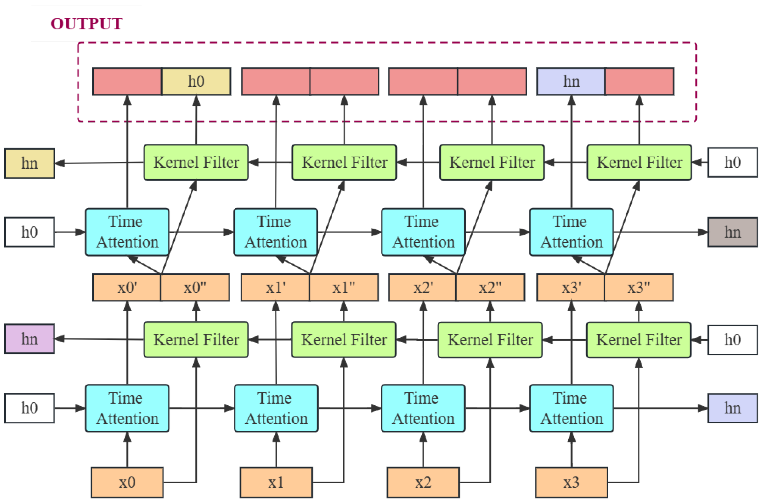
3.3.2. Time-Series Neural Network

The Time-series Neural Network (TNN) proposed in this study is a deep learning model designed for time-series prediction tasks. The design of this model fully considers the characteristics of time-series data, including time order, continuity, and periodicity, as shown in Figure 1. The network structure of TNN primarily comprises an input layer, hidden layers, and an output layer. The input layer receives raw time-series data, the hidden layers process these data using the Kernel Filter and Time Attention mechanism, and the output layer produces prediction results.

In the hidden layers of TNN, a multi-layer design is employed. This is because deep neural networks, through their multi-layer structure, can learn high-level features and abstract patterns from input data, which is beneficial for enhancing the model’s predictive performance. Specifically, the Kernel Filter is first used in the hidden layers to extract local patterns from the time-series data. Then, the Time Attention mechanism assigns weights to these patterns. Finally, the weighted features are passed to the next layer for further processing.

TNN has significant distinctions from regular deep neural networks (DNNs) when handling time-series data. Firstly, TNN designs the Kernel Filter and Time Attention operators, which can better handle the characteristics of time-series data, while regular DNNs often overlook these characteristics. Secondly, the number of layers and the network structure of TNN are optimized for time-series prediction tasks, while regular DNNs usually adopt a general network structure, which may not effectively handle time-series prediction tasks. Lastly, TNN can adaptively assign weights for each feature, while regular DNNs generally assume that all features are equally important. Furthermore, since the network structure of TNN is optimized for time-series prediction tasks, TNN can make more effective use of computational resources when handling large-scale time-series data, thereby enhancing prediction efficiency.

3.3.3. Kernel Filter

Kernel Filter represents an operator designed for the extraction of features from time-series data, with its primary objective being the isolation of key local patterns from the input time-series data. This section proceeds to detail the mathematical principles, design significance, conceptual source, and the specific application and advantages of the Kernel Filter within the Temporal Neural Network (TNN) model. The design of the Kernel Filter originates from the convolution operation within Convolutional Neural Networks (CNNs). In CNNs, the convolution kernel slides along the spatial dimension to extract local features from the input image. Drawing inspiration from this idea, the Kernel Filter was designed to slide along the temporal dimension, thereby extracting local patterns from time-series data.

The design carries several significant implications. Firstly, by applying convolutions along the temporal dimension, local patterns within time-series data can be captured, such as short-term fluctuations in stock prices. Secondly, different kernels can extract diverse features, enabling the model to understand time-series data from multiple perspectives. Finally, the convolution operation possesses the attribute of parameter sharing, implying that the same patterns can be sought throughout the entire time-series, an operation unachievable with traditional fully connected neural networks.

Within the TNN model, the Kernel Filter is responsible for the preliminary extraction of features from the input time-series data. Specifically, the model receives a segment of time-series data as input, which is initially processed by the Kernel Filter, resulting in a set of feature maps $\{h_1,h_2,\dots ,h_t\}$. These feature maps not only encapsulate local patterns of the time-series data but also preserve the temporal order of the data, providing abundant information for subsequent Time Attention. Its advantages in the tasks are clear. Firstly, since it can extract local patterns from time-series data, it enables the model to capture short-term fluctuations in stock prices, which is not achievable by traditional fully connected neural networks. Secondly, due to the parameter sharing attribute of the Kernel Filter, the model can seek the same patterns throughout the entire time-series, which is of significant importance for understanding and predicting stock prices. For a series of time-series data $\{x_1,x_2,\dots ,x_t\}$, a group of Kernel Filters $\{k_1,k_2,\dots ,k_n\}$ is defined; each kernel $k_i$ is a convolution kernel that can perform convolution on the input data along the temporal dimension, extracting local patterns from it. Each kernel $k_i$ consists of a group of weights $\{w_1^i,w_2^i,\dots ,w_d^i\}$ and a bias term $b_i$, where d is the size of the kernel. The operation of the Kernel Filter can be represented by the following formula:

$$h_t^i=f(\sum _{j=1}^d{w}_j^i·x_{t-j+1}+b_i)$$

(9)

In this formula, $h_t^i$ represents the output of the ith kernel at time t, and f is the activation function. When using the Kernel Filter, the size d and quantity n of the kernel need to be determined first. The size d of the kernel determines the time range of the patterns that can be captured, and the quantity n determines the diversity of the features that can be extracted. Then, at each time point t, each kernel convolves the input data to obtain the corresponding feature map $h_t^i$. Finally, all feature maps are integrated to obtain the final output of the Kernel Filter. Overall, the Kernel Filter extracts local patterns in time-series data through convolution operations, providing rich information for subsequent time-series prediction. Its design originates from the convolution operation of CNN, inherits the advantages of convolution operation in feature extraction, and overcomes the deficiencies of fully connected neural networks in handling time-series data, which is of great significance for the task.

3.3.4. Time Attention

Time attention is an operator designed for the allocation of feature weights in time-series data, as shown in Figure 2, with its main goal being to assign different weights to features at different time points, enabling the model to pay more attention to the features that have a significant impact on the prediction results. The mathematical principles, design significance, conceptual source, and specific application and advantages of time attention within the TNN model will be detailed in this section. The design of time attention originates from the idea of the Attention Mechanism. The primary concept of the Attention Mechanism is that when dealing with a task, the model should pay more attention to the information that has a larger impact on the results and pay less attention to information that has a smaller impact. Borrowing from this idea, time attention was designed to enable the model to pay more attention to the time points that have a larger impact on the prediction results when processing time-series data.

The design carries several important implications. Firstly, by assigning different weights to the features at each time point, the model can pay more attention to the features that have a larger impact on the prediction results, which is beneficial for improving the model’s prediction accuracy. Secondly, by introducing a weight generator, the model can automatically adjust the weights based on the input features, giving the model better adaptability. Lastly, the introduction of Time Attention allows the model to better consider the sequence and continuity of time when processing time-series data, which is not achievable with traditional fully connected neural networks.

In the TNN model, the main task of Time Attention is to assign different weights to the input feature sequence $\{h_1,h_2,\dots ,h_t\}$. To achieve this goal, a weight generator is designed which generates a weight ${\alpha }_t$ for the feature $h_t$ at each time point t. This weight generator is a small neural network, with the feature $h_t$ as input and the weight ${\alpha }_t$ as output. The specific operation of the weight generator can be represented by the following formula:

$${\alpha }_t=\sigma \left(g\left(h_t\right)\right)$$

(10)

In this formula, g is the weight generator, and $\sigma$ is a normalization function, which normalizes the generated weights so that the sum of all weights is 1. After obtaining the weight ${\alpha }_t$, the feature $h_t$ can be weighted to obtain the weighted feature ${\tilde{h}}_t$. The specific operation is as follows:

$${\tilde{h}}_t={\alpha }_t·h_t$$

(11)

Through this approach, distinct weights can be allocated to the features at each time point, enabling the model to focus on the features having a significant impact on the prediction outcomes. When employing Time Attention, the structure and parameters of the weight generator are first determined. Subsequently, the weight generator is utilized to generate a weight for each time point feature. This weight is then used to weight the feature, resulting in a weighted feature. Finally, all the weighted features are integrated to attain the final output of Time Attention.

Time Attention exhibits notable advantages in the tasks at hand. Firstly, by assigning different weights to the features at each time point, the model is better equipped to focus on the features that have a larger impact on the prediction results, contributing to an enhanced prediction accuracy of the model. Secondly, by introducing a weight generator, the model can auto-adjust the weights based on input features, thus granting the model improved adaptability. Finally, due to Time Attention’s superior consideration of the order and continuity of time, the model, when dealing with time-series data, possesses clear advantages over traditional fully connected neural networks. Compared to other attention mechanisms, Time Attention embodies important distinctions. To begin with, Time Attention is specifically designed for time-series data, providing a better consideration of the order and continuity of time, often overlooked by other attention mechanisms. Additionally, the weight generator in Time Attention is a small neural network capable of auto-adjusting weights based on the input features, granting Time Attention superior adaptability. In essence, by assigning distinct weights to the features at each time point, Time Attention enables the model to focus more effectively on the features impacting the prediction outcomes, will be discussed in Section 4. The design originates from the concept of the Attention Mechanism, inheriting its advantages in weight distribution while overcoming the shortcomings of traditional attention mechanisms when handling time-series data. Within the TNN model, Time Attention significantly enhances the model’s prediction accuracy and provides superior adaptability.

3.4. Experimental Settings

3.4.1. Experiment Designs

The initial problem addressed in this experimental design is the delineation of training and validation sets. Ordinarily, the entire dataset is divided into training and validation sets according to a specific ratio. The training set is primarily utilized for model training, where parameters are continuously adjusted and optimized through iterative learning of data in the training set. On the other hand, the validation set is mainly employed for evaluating the predictive performance of the model. By utilizing the validation set, the performance of the model on unseen data can be tested, thereby preventing overfitting of the training data. In this work, the split ratio adopted is 70% for the training set and 30% for the validation set.

To comprehensively evaluate the model’s performance, some baseline models are chosen for comparison. In this experiment, the following models are selected as baseline models: linear regression model [22], decision tree model [24], random forest model [33], support vector machine model [23], RNN [27], and LSTM [28]. These models are common in machine learning, have high practicality and wide applicability, and their predictive capabilities and model complexity can cover a wide range, making them good references to better evaluate the performance of the model.

Subsequently, validation experiments under different time slice spans are carried out. A time slice span refers to the selectable time unit when predicting future data. For example, days, weeks, or months can be chosen as the unit for predicting future data. Different time slice spans can affect the prediction accuracy and range of the model, making the choice of an appropriate time slice span crucial. In this experiment, the set of time slice spans is set to 1 day, 7 days, 30 days. For each time slice span, all the above-mentioned models are used for prediction, and their prediction results are recorded.

The experiments are conducted on a computing platform equipped with an Intel Core i9 processor, 64GB of RAM, and an NVIDIA RTX 3090 GPU. The software environment consisted of Python 3.8, PyTorch 1.9, and various other supporting Python libraries. For the TNN models, we employed three major filters: Squeeze-and-Excitation Networks (SENets), Convolutional Block Attention Module (CBAM), and Kalman Filters based on mentioned libraries. It is essential to note that there are no “official” third-party libraries available for these filters. Therefore, we implemented these algorithms from scratch in PyTorch by carefully referencing their respective official papers [34,35,36].

3.4.2. Evaluation Metric

Model evaluation metrics are important tools for measuring model prediction capabilities, and commonly used metrics include the Root Mean Square Error (RMSE), Mean Absolute Error (MAE), Mean Absolute Percentage Error (MAPE), and Coefficient of Determination ($R^2$). The calculation methods, the significance in this research task, and the model capabilities reflected by these metrics are explained in detail below.

Firstly, the Root Mean Square Error (RMSE) is a common model evaluation metric used to measure the bias between the model’s predictions and the actual values. Its formula is as follows:

$$RMSE=\sqrt{\frac{1}{n}\sum _{i=1}^n{(y_i-{\widehat{y}}_i)}^2}$$

(12)

Here, n is the total number of samples, $y_i$ is the actual value of the $i^{th}$ sample, and ${\widehat{y}}_i$ is the model’s prediction for the $i^{th}$ sample. In this work, RMSE can accurately evaluate the accuracy of the model’s prediction of time-series data. The smaller the RMSE value, the smaller the bias between the model’s predictions and the actual results, indicating a higher prediction accuracy of the model. It is worth noting that RMSE gives more weight to larger errors, so if the model’s predictions have large deviations, the RMSE value will increase accordingly.

Secondly, the Mean Absolute Error (MAE) is another evaluation metric for model prediction capabilities. Unlike RMSE, MAE pays more attention to the average bias between the model’s predictions and the actual results rather than the variance of the predictions. Its formula is as follows:

$$MAE=\frac{1}{n}\sum _{i=1}^n|y_i-{\widehat{y}}_i|$$

(13)

In this formula, n is the total number of samples, $y_i$ is the actual value of the $i^{th}$ sample, and ${\widehat{y}}_i$ is the model’s prediction for the $i^{th}$ sample. In this research task, using MAE can more intuitively reflect the average deviation between the model’s predictions and the actual results. The smaller the MAE value, the smaller the bias between the model’s predictions and the actual results, indicating a higher prediction accuracy of the model. Compared to RMSE, MAE gives equal weight to all errors, so when the model’s predictions have large deviations, the MAE value will be relatively smaller.

The Mean Absolute Percentage Error (MAPE) is an evaluation metric that provides a percentage-based representation of the errors between predicted and actual values, offering an easy-to-interpret scale of accuracy. The formula for calculating MAPE is as follows:

$$MAPE=\frac{1}{n}\sum _{i=1}^n\left|\frac{y_i-{\widehat{y}}_i}{y_i}\right|$$

(14)

In this formula, n is the total number of samples, $y_i$ is the actual value of the $i^{th}$ sample, and ${\widehat{y}}_i$ is the model’s prediction for the $i^{th}$ sample. The smaller the MAPE value, the higher the model’s prediction accuracy. One of the advantages of using MAPE is that it provides an easily interpretable percentage error, enabling the performance of the model to be understood in a straightforward manner.

Finally, the Coefficient of Determination ($R^2$) is an evaluation metric that reflects the correlation between the model’s predictions and the actual results. The closer $R^2$ is to 1, the higher the correlation between the model’s predictions and the actual results. Its formula is as follows:

$$R^2=1-\frac{{\sum }_{i=1}^n{(y_i-{\widehat{y}}_i)}^2}{{\sum }_{i=1}^n{(y_i-\overline{y})}^2}$$

(15)

In this formula, n is the total number of samples, $y_i$ is the actual value of the $i^{th}$ sample, ${\widehat{y}}_i$ is the model’s prediction for the $i^{th}$ sample, and $\overline{y}$ is the mean of the actual values. In this research task, $R^2$ can be used to evaluate the correlation between the model’s predictions and the actual results. The higher the $R^2$ value, the higher the correlation between the model’s predictions and the actual results, indicating a higher prediction accuracy of the model.

In summary, through the above model evaluation metrics, the predictive capabilities of the model can be comprehensively evaluated from different angles. RMSE focuses more on the variance of the model’s predictions, MAE focuses more on the average bias between the model’s predictions and the actual results, MAPE offers a percentage-based representation of the model’s prediction errors, providing an easily interpretable scale for assessing the model’s accuracy, and $R^2$ evaluates the correlation between the model’s predictions and the actual results. These metrics are important tools for measuring model prediction capabilities and can effectively help in understanding and improving the predictive performance of the model.

4. Results and Discussion

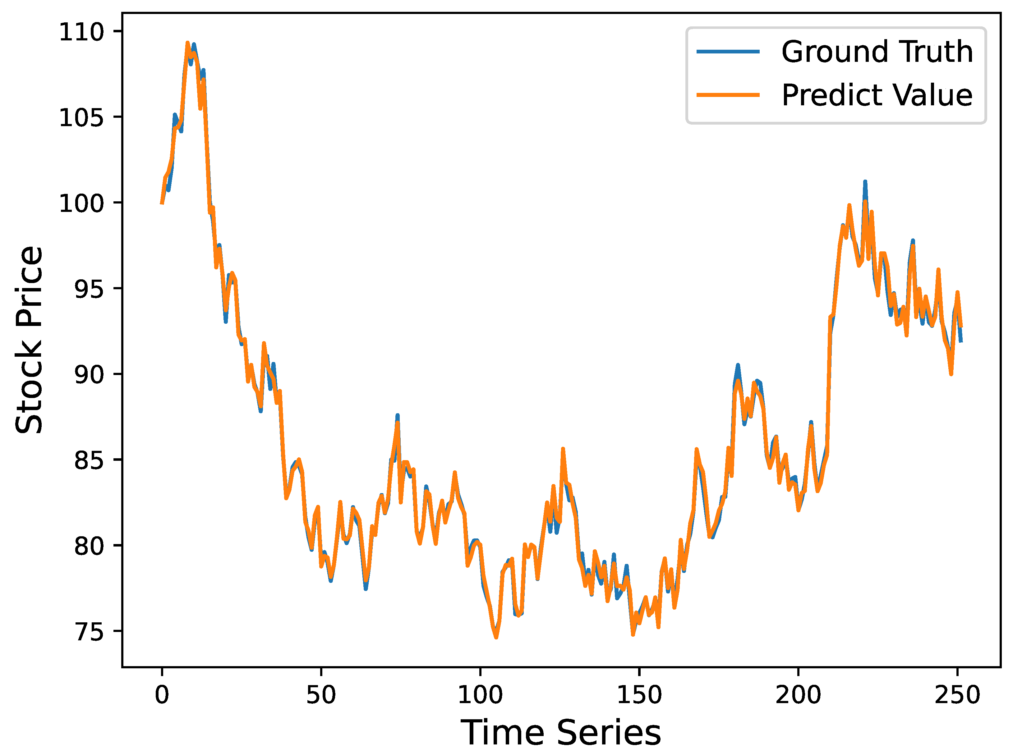
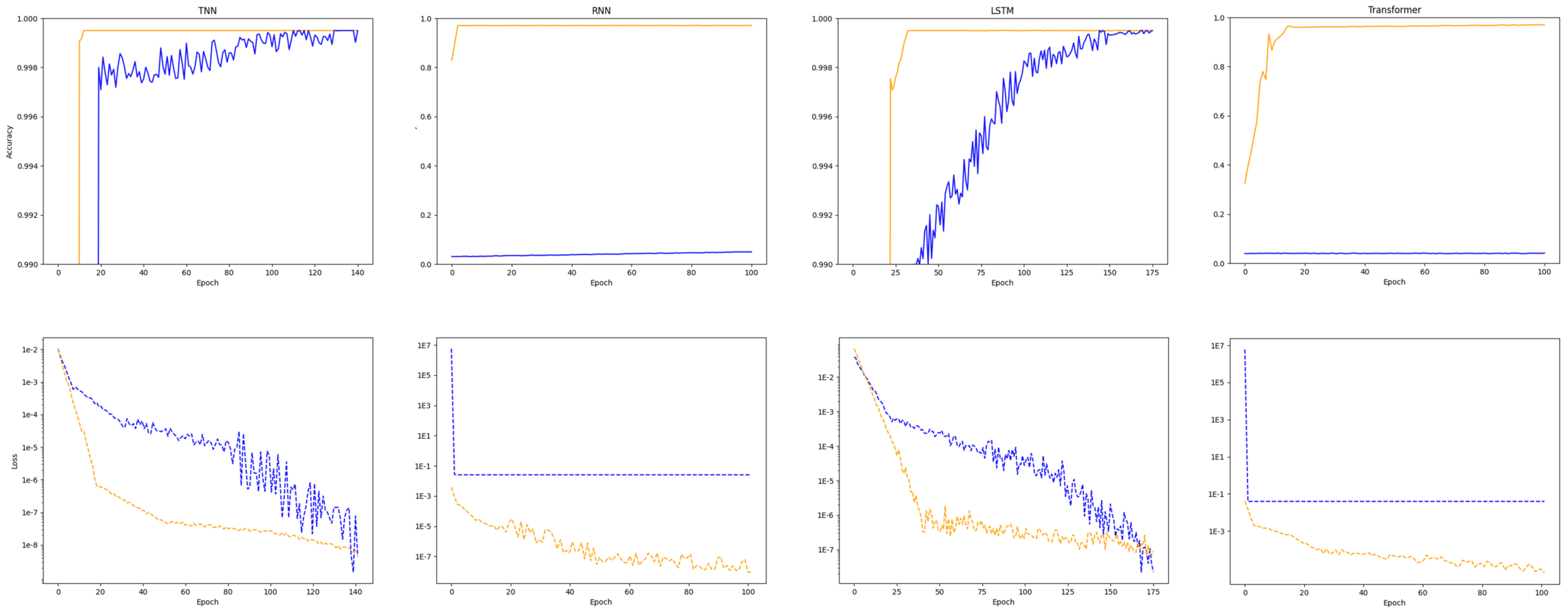
4.1. Results of Time Series Forecasting

The primary objective of this experiment is to conduct stock price prediction using various machine learning models and compare their predictive performance. To realize this goal, different time spans (1 day, 7 days, 30 days) were set, and seven distinct models, including TNN, linear regression, decision tree, random forest, SVM, RNN, and LSTM, were utilized. The predictive performance of each model across all time spans was assessed by computing the RMSE, MAE, and coefficient of determination ($R^2$).

From the results tabulated in

Table 1. Results of S&P 500 price in different periods.

Model	Time Span	RMSE	MAE	${\mathit{R}}^2$	MAPE
TNN	1 day	0.05	0.23	0.95	1.3%
Linear Regression	1 day	0.34	0.57	0.63	7.5%
Decision Tree	1 day	0.36	0.60	0.61	7.8%
Random Forest	1 day	0.21	0.47	0.69	5.1%
SVM	1 day	0.23	0.48	0.67	4.1%
RNN	1 day	0.13	0.37	0.87	2.8%
LSTM	1 day	0.09	0.3	0.91	1.9%
TNN	7 day	0.16	0.4	0.89	1.8%
Linear Regression	7 day	0.67	0.81	0.35	9.6%
Decision Tree	7 day	0.65	0.81	0.39	8.9%
Random Forest	7 day	0.56	0.75	0.43	6.3%
SVM	7 day	0.49	0.70	0.47	5.8%
RNN	7 day	0.25	0.50	0.61	3.3%
LSTM	7 day	0.23	0.48	0.66	3.1%
TNN	30 day	0.14	0.37	0.91	3.7%
Linear Regression	30 day	0.85	0.92	0.16	11.2%
Decision Tree	30 day	0.82	0.90	0.20	13.9%
Random Forest	30 day	0.77	0.88	0.29	10.4%
SVM	30 day	0.76	0.88	0.29	6.8%
RNN	30 day	0.27	0.52	0.63	4.9%
LSTM	30 day	0.28	0.53	0.58	3.7%

, it is observable that the TNN model performed the best across all time spans, having the lowest RMSE and MAE, and the highest $R^2$, which is also shown in Figure 3. Upon further discussion, the sectors with the highest prediction accuracy in the S&P 500 are Technology, Healthcare, Financials, and Communication Services, followed by Basic Materials and Consumer Staples. The sectors with the lowest accuracy are Consumer Discretionary, Industrials, and Energy. This disparity in predictive accuracy across sectors could potentially be attributed to the intrinsic volatility and complexity of certain sectors compared to others. Specifically, sectors like Consumer Discretionary, Industrials, and Energy tend to be more volatile and are influenced by a wide array of external factors, making them harder to accurately predict. This indicates that the TNN model exhibited a high degree of precision in stock price prediction, with minimal deviation from the actual results, and a high correlation between the predicted and actual outcomes. This can potentially be attributed to the strong feature extraction capability of the TNN model, which can extract useful information from raw data, thereby enhancing the predictive accuracy of the model. In the case of the other models, it was noted that as the time span increased, the performance of the models generally decreased, i.e., RMSE and MAE increased while $R^2$ decreased. This could be due to the increase in future uncertainties with the extension of the time span, leading to a drop in predictive performance. However, the RNN and LSTM models demonstrated a lesser degree of performance reduction with increased time spans compared to other models. This could be attributed to the fact that both RNN and LSTM models are sequence models capable of handling time-series data, thus outperforming other models in long-term trend prediction.

A deeper analysis of the experimental results from the characteristics and mathematical theories of each model was subsequently undertaken. Firstly, the Linear Regression model exhibited the poorest predictive performance among all models. This is likely because stock price fluctuations are influenced by numerous factors, including macroeconomic conditions, company financials, and market sentiment, among others. The complex and non-linear relationships between these factors make it challenging for linear models to accurately capture these relationships. The Decision Tree and Random Forest models were next in the analysis, both being tree-structured models with excellent interpretability. However, their predictive performance left room for improvement. This might be due to the fact that while they can handle non-linear relationships, they struggle with time-series data as they cannot capture time dependency within the data. SVM, a model based on margin maximization, demonstrated better predictive performance than Linear Regression, Decision Tree, and Random Forest. However, its performance still lagged behind RNN, LSTM, and TNN. This might be because while SVM can handle non-linear problems, it may struggle with the “curse of dimensionality” when dealing with high-dimensional, complex time-series data. Lastly, the RNN and LSTM models, both types of recurrent neural networks, are especially adept at handling time-series data. RNN and LSTM can capture time dependency in data, hence performing better in stock price prediction than other models. Particularly, LSTM, due to its inherent design advantages, can overcome the gradient vanishing and exploding problems faced by RNN, thereby demonstrating slightly superior predictive performance.

4.2. Test on Different Attention Mechanisms

The objective of this experimental design was to evaluate the performance of various attention mechanisms in predicting the S&P 500 index prices. The aim is to understand the effectiveness and applicability of different attention mechanisms specifically in the domain of stock price forecasting.

Focusing on the experimental results in

Table 2. Results of different attention mechanisms.

Attention Model	RMSE	MAE	${\mathit{R}}^2$
SENet [34]	0.08	0.27	0.87
CBAM [35]	0.09	0.3	0.92
Time Attention	0.05	0.23	0.95

, it is clear that the Time Attention model outperformed the other attention mechanisms across all metrics. This adds empirical evidence to the model’s theoretical advantages in capturing time-dependent features. The TNN model, which incorporates the Time Attention mechanism, yielded the lowest RMSE and MAE values and the highest $R^2$ score, demonstrating its superior predictive accuracy and stability in stock price prediction. Specifically, SENet and CBAM, despite being effective attention mechanisms, fell short in capturing temporal complexities inherent in stock market data. This is reflected in their lower $R^2$ values compared to the Time Attention model. While SVM, RNN, and LSTM also performed better than traditional machine learning models like Linear Regression and Decision Trees, they were still outperformed by the TNN model. Interestingly, the data suggest that the ability to capture time-dependent features effectively separates TNN from other models, justifying its superior performance in our experimental setup.

In summary, the comparative evaluation of different models based on our dataset provides concrete evidence that attention mechanisms, particularly Time Attention, can significantly enhance the accuracy and reliability of stock price predictions. This suggests that future research in this area could benefit substantially from the integration of time-sensitive attention mechanisms.

4.3. Test on Kernel Filter

The principal objective of this experiment is to scrutinize the effectiveness of different filters applied within the TNN, and thus underscore the significance of the Kernel Filter in enhancing the precision of time-series forecasting. To be specific, three distinct model configurations were compared in the experiment: a TNN model devoid of filters, a TNN model equipped with a Kalman Filter [36], and a TNN model furnished with a Kernel Filter.

As illustrated in

Table 3. Results of different filters.

Model	RMSE	MAE	${\mathit{R}}^2$
TNN (No Filter)	0.26	0.51	0.82
TNN (Kalman Filter)	0.12	0.34	0.91
TNN (Kernel Filter)	0.05	0.23	0.95

, the TNN model with no filter yielded RMSE, MAE, and $R^2$ values of 0.26, 0.51, and 0.82, respectively. These findings indicate that the TNN model can produce satisfactory predictions even without any filter, primarily due to the inherent advantages of the TNN model structure. This model is capable of attributing different weights to features at each timestamp, thereby enabling a focused approach towards features with significant impacts on the predictions. However, in the absence of a filter, the model may encounter challenges when handling complex, noisy time-series data, leading to a potential compromise in the predictive performance. In contrast, the TNN model employing the Kalman Filter demonstrated RMSE, MAE, and $R^2$ values of 0.12, 0.34, and 0.91, respectively, revealing a marked enhancement in predictive performance with the inclusion of the Kalman Filter. The Kalman Filter, characterized as a linear filter, can accurately estimate system states amidst noisy data, consequently boosting the model’s predictive accuracy to a certain extent. However, being linear, the Kalman Filter might fall short when faced with complex non-linear time-series data. Lastly, the TNN model incorporating the Kernel Filter exhibited RMSE, MAE, and $R^2$ values of 0.05, 0.23, and 0.95, respectively. Evidently, the introduction of the Kernel Filter further improved the predictive performance of the TNN model, outperforming the other two model configurations across all metrics. This superior performance primarily results from the impressive capabilities of the Kernel Filter. Compared to the Kalman Filter, the Kernel Filter can handle not only noisy data but also non-linear time-series data effectively. Its proficiency in extracting higher-level features from time-series data surpasses that of the Kalman Filter, as shown in Figure 4. Therefore, the introduction of the Kernel Filter enables the TNN model to achieve higher prediction accuracy when dealing with complex time-series data.

4.4. Limitations and Future Work

Despite the progress and achievements made in this research, the model does have some limitations that suggest avenues for future work. For example, while the model performs well on certain datasets, it can struggle with time-series data containing substantial noise. Additionally, its treatment of time slice spans lacks flexibility, which is an issue for varying real-world applications. Moreover, the model’s current capability does not fully address the intercorrelation between features or offer a comprehensive set of evaluation metrics. These limitations outline the areas where improvements are needed:

• Noise Handling: To mitigate the issue of noise, future research will incorporate various noise filtering and denoising techniques like Kalman filters and median filters.
• Time Slice Flexibility: Future versions of the model will aim to allow dynamic adjustments of time slice spans to meet different application requirements, thereby increasing the model’s adaptability.
• Feature Correlations: Efforts will be undertaken to better uncover and incorporate the intercorrelations among features, with the goal of improving prediction accuracy.
• Evaluation Criteria: Additional metrics such as stability, robustness, and computational efficiency will be introduced to provide a more rounded evaluation of the model’s performance.
• Extended Capabilities: The TNN model will be further developed to capture not just time dependencies but also more complex relationships dependent on the history of changes in incoming parameters, making it more versatile for different types of time-series prediction tasks.

Through targeted advancements in these areas, the model is expected to become more robust and versatile, better serving the complex and varying demands of practical applications.

5. Conclusions

The theme of this research is centered on a high-accuracy time-series forecasting method known as the TNN, which is based on a Kernel Filter and Time Attention mechanism. Forecasting analysis of time-series data is a crucial task in various domains. Nevertheless, high-precision time-series forecasting remains a challenge due to inherent complexities such as non-linearity, high dimensionality, and long-term dependencies. To overcome these challenges, a novel Time Neural Network model has been designed and implemented in this study.

The major innovation of the TNN model involves the introduction of a Time Attention mechanism and a Kernel Filter. The Time Attention mechanism allows the model to allocate different weights to the features at each time point, enabling the model to focus more on features that have a significant impact on the forecasting results. Meanwhile, the Kernel Filter is used to extract high-level features from time-series data, thereby improving the prediction accuracy of the model. In addition, an adaptive weight generator is incorporated into the model, allowing it to automatically adjust the weights according to the input features.

In the experimental section, several mainstream time-series forecasting models, including RNN and LSTM, were adopted as baseline models, and exhaustive comparative experiments were conducted. The results demonstrate that the TNN model significantly outperforms the baseline models, regardless of whether the forecasting tasks are short-term or long-term. Importantly, even for complex time-series data containing a large amount of noise, the TNN model is still capable of maintaining high prediction accuracy. Ablation experiments validated the crucial contribution of the Time Attention mechanism and Kernel Filter to the performance of the model. When either the Time Attention mechanism or Kernel Filter is removed, a significant decline in the predictive performance of the model is evident, further underscoring the importance of these two components in the model.

Despite the excellent performance of the TNN model in the experiments, certain limitations remain. These include the need for enhanced noise data processing capabilities, flexibility in dealing with different time slice spans, and comprehensive handling of the interrelatedness among features. Future work will focus on improving and deepening the approach to address these issues.

In conclusion, the TNN model proposed in this study provides a novel solution for time-series forecasting. By incorporating a Time Attention mechanism and Kernel Filter, the model demonstrates superior forecasting performance and adaptability when dealing with complex time-series data. Despite some existing limitations, it is believed that through future improvements and in-depth exploration, the TNN model can play a greater role in the field of time-series forecasting, offering more accurate and reliable predictions for real-world problem solving.

References

1. Zhang, Y.; Wang, H.; Xu, R.; Yang, X.; Wang, Y.; Liu, Y. High-Precision Seedling Detection Model Based on Multi-Activation Layer and Depth-Separable Convolution Using Images Acquired by Drones. Drones 2022, 6, 152. [Google Scholar] [CrossRef]
2. Lin, X.; Wa, S.; Zhang, Y.; Ma, Q. A dilated segmentation network with the morphological correction method in farming area image Series. Remote Sens. 2022, 14, 1771. [Google Scholar] [CrossRef]
3. Zhang, Y.; Liu, X.; Wa, S.; Liu, Y.; Kang, J.; Lv, C. GenU-Net++: An Automatic Intracranial Brain Tumors Segmentation Algorithm on 3D Image Series with High Performance. Symmetry 2021, 13, 2395. [Google Scholar] [CrossRef]
4. Zhang, Y.; He, S.; Wa, S.; Zong, Z.; Lin, J.; Fan, D.; Fu, J.; Lv, C. Symmetry GAN Detection Network: An Automatic One-Stage High-Accuracy Detection Network for Various Types of Lesions on CT Images. Symmetry 2022, 14, 234. [Google Scholar] [CrossRef]
5. Maarif, M.R.; Saleh, A.R.; Habibi, M.; Fitriyani, N.L.; Syafrudin, M. Energy Usage Forecasting Model Based on Long Short-Term Memory (LSTM) and eXplainable Artificial Intelligence (XAI). Information 2023, 14, 265. [Google Scholar] [CrossRef]
6. Huo, H.; Guo, J.; Yang, X.; Lu, X.; Wu, X.; Li, Z.; Li, M.; Ren, J. An Accelerated Method for Protecting Data Privacy in Financial Scenarios Based on Linear Operation. Appl. Sci. 2023, 13, 1764. [Google Scholar] [CrossRef]
7. Manfre Jaimes, D.; Manuel Zamudio López, M.; Zareipour, H.; Quashie, M. A Hybrid Model for Multi-Day-Ahead Electricity Price Forecasting considering Price Spikes. Forecasting 2023, 5, 499–521. [Google Scholar] [CrossRef]
8. Ampountolas, A. Comparative Analysis of Machine Learning, Hybrid, and Deep Learning Forecasting Models: Evidence from European Financial Markets and Bitcoins. Forecasting 2023, 5, 472–486. [Google Scholar] [CrossRef]
9. Sedai, A.; Dhakal, R.; Gautam, S.; Dhamala, A.; Bilbao, A.; Wang, Q.; Wigington, A.; Pol, S. Performance Analysis of Statistical, Machine Learning and Deep Learning Models in Long-Term Forecasting of Solar Power Production. Forecasting 2023, 5, 256–284. [Google Scholar] [CrossRef]
10. Wood, M.; Ogliari, E.; Nespoli, A.; Simpkins, T.; Leva, S. Day Ahead Electric Load Forecast: A Comprehensive LSTM-EMD Methodology and Several Diverse Case Studies. Forecasting 2023, 5, 297–314. [Google Scholar] [CrossRef]
11. Mishra, A.; Dasgupta, A. Supervised and Unsupervised Machine Learning Algorithms for Forecasting the Fracture Location in Dissimilar Friction-Stir-Welded Joints. Forecasting 2022, 4, 787–797. [Google Scholar] [CrossRef]
12. Papadimitriou, T.; Gogas, P.; Athanasiou, A.F. Forecasting Bitcoin Spikes: A GARCH-SVM Approach. Forecasting 2022, 4, 752–766. [Google Scholar] [CrossRef]
13. Fianu, E.S. Analyzing and Forecasting Multi-Commodity Prices Using Variants of Mode Decomposition-Based Extreme Learning Machine Hybridization Approach. Forecasting 2022, 4, 538–564. [Google Scholar] [CrossRef]
14. Carrillo, J.A.; Nieto, M.; Velez, J.F.; Velez, D. A New Machine Learning Forecasting Algorithm Based on Bivariate Copula Functions. Forecasting 2021, 3, 355–376. [Google Scholar] [CrossRef]
15. Yasrab, R.; Jiang, W.; Riaz, A. Fighting Deepfakes Using Body Language Analysis. Forecasting 2021, 3, 303–321. [Google Scholar] [CrossRef]
16. May, M.C.; Albers, A.; Fischer, M.D.; Mayerhofer; Florian an Schäfer, L.; Lanza, G. Queue Length Forecasting in Complex Manufacturing Job Shops. Forecasting 2021, 3, 322–338. [Google Scholar] [CrossRef]
17. Rezazadeh, A. A Generalized Flow for B2B Sales Predictive Modeling: An Azure Machine-Learning Approach. Forecasting 2020, 2, 267–283. [Google Scholar] [CrossRef]
18. Claveria, O. Forecasting with Business and Consumer Survey Data. Forecasting 2021, 3, 113–134. [Google Scholar] [CrossRef]
19. Shah, V.H. Machine learning techniques for stock prediction. Found. Mach. Learn. Spring 2007, 1, 6–12. [Google Scholar]
20. Janiesch, C.; Zschech, P.; Heinrich, K. Machine learning and deep learning. Electron. Mark. 2021, 31, 685–695. [Google Scholar] [CrossRef]
21. Murphy, K.P. Probabilistic Machine Learning: An Introduction; MIT Press: Cambridge, MA, USA, 2022. [Google Scholar]
22. Maulud, D.; Abdulazeez, A.M. A review on linear regression comprehensive in machine learning. J. Appl. Sci. Technol. Trends 2020, 1, 140–147. [Google Scholar] [CrossRef]
23. Hearst, M.A.; Dumais, S.T.; Osuna, E.; Platt, J.; Scholkopf, B. Support vector machines. IEEE Intell. Syst. Their Appl. 1998, 13, 18–28. [Google Scholar] [CrossRef]
24. Wan, A.; Dunlap, L.; Ho, D.; Yin, J.; Lee, S.; Jin, H.; Petryk, S.; Bargal, S.A.; Gonzalez, J.E. NBDT: Neural-backed decision trees. arXiv 2020, arXiv:2004.00221. [Google Scholar]
25. Kurani, A.; Doshi, P.; Vakharia, A.; Shah, M. A comprehensive comparative study of artificial neural network (ANN) and support vector machines (SVM) on stock forecasting. Ann. Data Sci. 2023, 10, 183–208. [Google Scholar] [CrossRef]
26. Ma, Y.; Han, R.; Fu, X. Stock prediction based on random forest and LSTM neural network. In Proceedings of the 2019 19th International Conference on Control, Automation and Systems (ICCAS), Jeju, Republic of Korea, 15–18 October 2019; pp. 126–130. [Google Scholar]
27. Zaremba, W.; Sutskever, I.; Vinyals, O. Recurrent neural network regularization. arXiv 2014, arXiv:1409.2329. [Google Scholar]
28. Graves, A.; Graves, A. Long short-term memory. In Supervised Sequence Labelling with Recurrent Neural Networks; Springer: Berlin/Heidelberg, Germany, 2012; pp. 37–45. [Google Scholar]
29. Zhao, J.; Zeng, D.; Liang, S.; Kang, H.; Liu, Q. Prediction model for stock price trend based on recurrent neural network. J. Ambient. Intell. Humaniz. Comput. 2021, 12, 745–753. [Google Scholar] [CrossRef]
30. Zhu, Y. Stock price prediction using the RNN model. J. Phys. Conf. Ser. 2020, 1650, 032103. [Google Scholar] [CrossRef]
31. Swathi, T.; Kasiviswanath, N.; Rao, A.A. An optimal deep learning-based LSTM for stock price prediction using twitter sentiment analysis. Appl. Intell. 2022, 52, 13675–13688. [Google Scholar] [CrossRef]
32. Ma, Q. Comparison of ARIMA, ANN and LSTM for stock price prediction. In Proceedings of the E3S Web of Conferences, Chongqing, China, 20–22 November 2020; Volume 218, p. 01026. [Google Scholar]
33. Li, Y.; Zou, C.; Berecibar, M.; Nanini-Maury, E.; Chan, J.C.W.; Van den Bossche, P.; Van Mierlo, J.; Omar, N. Random forest regression for online capacity estimation of lithium-ion batteries. Appl. Energy 2018, 232, 197–210. [Google Scholar] [CrossRef]
34. Hu, J.; Shen, L.; Sun, G. Squeeze-and-Excitation Networks. In Proceedings of the 2018 IEEE/CVF Conference on Computer Vision and Pattern Recognition, Salt Lake City, UT, USA, 18–23 June 2018; pp. 7132–7141. [Google Scholar] [CrossRef]
35. Woo, S.; Park, J.; Lee, J.; Kweon, I.S. CBAM: Convolutional Block Attention Module. CoRR 2018. Available online: http://xxx.lanl.gov/abs/1807.06521 (accessed on 6 September 2023).
36. Kalman, R.E. A new approach to linear filtering and prediction problems. J. Basic Eng. Mar. 1960, 82, 35–45. [Google Scholar] [CrossRef]
37. Vaswani, A.; Shazeer, N.; Parmar, N.; Uszkoreit, J.; Jones, L.; Gomez, A.N.; Kaiser, Ł.; Polosukhin, I. Attention is all you need. Adv. Neural Inf. Process. Syst. 2017, 30. Available online: https://proceedings.neurips.cc/paper_files/paper/2017/file/3f5ee243547dee91fbd053c1c4a845aa-Paper.pdf (accessed on 6 September 2023).
Figure 1. Illustration of the time-series neural network structure.
Information 14 00500 g001
Figure 2. Illustration of time attention structure.
Information 14 00500 g002
Figure 3. Ground truth and the predicted values by TNN.
Information 14 00500 g003
Figure 4. Comparison of different filters on RNN, LSTM, Transformer [37], and ours. The orange line denotes the performance for different models with Kernel Filter, while the blue one is that without Kernel Filter.
Information 14 00500 g004