
Enhancing Network Intrusion Detection: A Genetic Programming Symbolic Classifier Approach


Faculty of Engineering, University of Rijeka, Vukovarska 58, 51000 Rijeka, Croatia
*
Author to whom correspondence should be addressed.
†
These authors contributed equally to this work.
Information 2024, 15(3), 154; https://0-doi-org.brum.beds.ac.uk/10.3390/info15030154
Submission received: 5 February 2024
/
Revised: 29 February 2024
/
Accepted: 7 March 2024
/
Published: 9 March 2024
(This article belongs to the Special Issue Advanced Computer and Digital Technologies)
Abstract
:This investigation underscores the paramount imperative of discerning network intrusions as a pivotal measure to fortify digital systems and shield sensitive data from unauthorized access, manipulation, and potential compromise. The principal aim of this study is to leverage a publicly available dataset, employing a Genetic Programming Symbolic Classifier (GPSC) to derive symbolic expressions (SEs) endowed with the capacity for exceedingly precise network intrusion detection. In order to augment the classification precision of the SEs, a pioneering Random Hyperparameter Value Search (RHVS) methodology was conceptualized and implemented to discern the optimal combination of GPSC hyperparameter values. The GPSC underwent training via a robust five-fold cross-validation regimen, mitigating class imbalances within the initial dataset through the application of diverse oversampling techniques, thereby engendering balanced dataset iterations. Subsequent to the acquisition of SEs, the identification of the optimal set ensued, predicated upon metrics inclusive of accuracy, area under the receiver operating characteristics curve, precision, recall, and F1-score. The selected SEs were subsequently subjected to rigorous testing on the original imbalanced dataset. The empirical findings of this research underscore the efficacy of the proposed methodology, with the derived symbolic expressions attaining an impressive classification accuracy of 0.9945. If the accuracy achieved in this research is compared to the average state-of-the-art accuracy, the accuracy obtained in this research represents the improvement of approximately 3.78%. In summation, this investigation contributes salient insights into the efficacious deployment of GPSC and RHVS for the meticulous detection of network intrusions, thereby accentuating the potential for the establishment of resilient cybersecurity defenses.
1. Introduction
Network intrusion detection assumes paramount significance in ensuring the security and integrity of computer networks within our contemporary interconnected and digital milieu [1]. It plays an integral role in the identification and prevention of malicious activities that pose threats to the confidentiality, availability, and integrity of sensitive information and digital resources.
Primarily, network intrusion detection is indispensable for the identification and mitigation of diverse cyber threats, encompassing malware, ransomware, and unauthorized access attempts [2]. Through the meticulous analysis of network traffic patterns and the vigilant monitoring of system logs, intrusion detection systems (IDSs) [3] can discern unusual or suspicious activities indicative of a potential security breach. Such early detection empowers security teams to respond promptly, thereby minimizing the potential damage inflicted by cyber attacks.
Secondarily, network intrusion detection plays a pivotal role in aiding organizations to conform to stringent regulatory requirements and industry standards [4]. Various sectors, including finance, healthcare, and government, are subject to rigorous regulations governing the protection of sensitive data. The implementation of effective intrusion detection systems serves to showcase organizational commitment to security and compliance, thereby mitigating the risks of legal and financial repercussions associated with data breaches [5].
Moreover, network intrusion detection contributes substantively to the overarching risk management strategy of an organization. By identifying vulnerabilities and potential security weaknesses, intrusion detection systems facilitate proactive measures to fortify the network’s defenses [6]. This includes addressing software vulnerabilities through timely patching, updating security policies, and implementing additional security controls to mitigate the risk of future cyber threats.
Additionally, the significance of network intrusion detection extends to the monitoring of insider threats and employee activities within an organization. The manifestation of malicious insider actions or unintentional security lapses by employees poses considerable risks to an organization’s security [7]. Intrusion detection systems prove invaluable in detecting abnormal user behavior or unauthorized access attempts, affording organizations the ability to investigate and address potential insider threats.
In summary, network intrusion detection stands as a foundational component of a comprehensive cybersecurity strategy, providing continuous monitoring and analysis of network traffic for the real-time detection and response to cyber threats [8]. This proactive approach is essential for safeguarding sensitive information, maintaining regulatory compliance, and protecting the overall well-being of an organization amidst the ever-evolving landscape of cyber threats.
The utilization of artificial intelligence (AI) in network intrusion detection becomes imperative due to its efficacy in enhancing the efficiency and accuracy of threat detection within complex and dynamic cyber environments. AI-powered intrusion detection systems harness machine learning algorithms to scrutinize extensive network data, identifying patterns and anomalies indicative of potential security breaches. Unlike traditional signature-based systems, AI-driven solutions exhibit adaptability and learning capabilities, thereby offering a proactive defense against sophisticated and previously unknown cyber attacks. This enables organizations to stay ahead of evolving threats, minimize false positives, and respond more effectively to emerging security challenges, ultimately fortifying the resilience of their network infrastructure in the face of constantly evolving cyber risks.
Furthermore, various studies have explored the application of Artificial Neural Networks (ANNs) in the detection of malicious network traffic [9]. One such investigation employed the 10-fold cross-validation technique for ANN training, achieving an accuracy (ACC) of 0.98 and an area under the receiver operator characteristic curve (AUC) of 0.98 [9]. In another study, the UNSW-NB15 dataset and the original dataset were employed to train a Convolutional Neural Network (CNN) for multiclass classification, achieving an accuracy of 0.956 [10]. Support vector classifiers (SVCs) and extreme learning machines (ELMs) were utilized for network intrusion detection in conjunction with a modified K-Means method for feature extraction, yielding a highest estimation accuracy of 0.9575 [11]. An ensemble method, comprising Naive Bayes, PART, and Adaptive Boost, was employed for network intrusion detection, achieving the highest accuracy (ACC) of 0.9997 [12]. Similarly, a multi-layer ensemble method utilizing SVC was applied for network intrusion detection and classification, coupled with a Deep Belief Network for feature extraction, resulting in the highest classification accuracy (ACC) of 0.9727 [13]. Principal component analysis (PCA) and Auto-Encoder were employed for feature extraction, and a CNN was utilized for the detection of network intrusion types in yet another study, achieving the highest accuracy (ACC) of 0.94 [14].
The authors in [15] used recurrent neural networks (RNNs) for network intrusion type detection and compared the classification performance to that achieved with J48, ANN, random forest (RFC) and SVC. In this case, the RNN achieved the highest classification accuracy of 0.9709. The ensemble method based on selection using the Bat algorithm was used in [16] for the detection of the network intrusion type, and the highest accuracy achieved was 0.98944. A nonsymmetric deep auto encoder with random forest classifier was used [17] for network intrusion detection on KDD Cup 99 and NSL-KDD benchmark datasets. The highest classification accuracy achieved in this case was 0.979 on the KDD Cup 99 dataset. Deep learning neural networks (DNNs) have been used in [18,19] for network intrusion detection, and the highest classification accuracy results achieved in both cases were 0.9995 and 0.9938, respectively.
The reinforcement learning methods have also been used for network intrusion detection [20,21]. In [21], deep Q-learning was used for the detection of different types of network intrusions. The highest accuracy achieved with this model was 0.78.
The results of the previously discussed research are summarized in Table 1.
From the findings presented in Table 1, it becomes evident that a predominant number of scholarly works have employed neural networks, specifically Artificial Neural Networks (ANNs) and Convolutional Neural Networks (CNNs), for the purpose of network intrusion detection. In certain investigations, sophisticated ensemble methods have been incorporated alongside ANN/CNN methodologies. Remarkably, all these methodologies have exhibited exemplary levels of detection and classification performance. However, a critical limitation of these approaches lies in their inherent complexity, rendering them resistant to facile transformation into succinct symbolic expressions (SEs). Furthermore, the exigent computational demands for training, storage, and reutilization pose an additional challenge for these AI methods.
This paper endeavors to surmount these challenges by deploying the Genetic Programming Symbolic Classifier (GPSC) method on a publicly available dataset. The aim is to derive symbolic expressions (SEs) possessing the capacity for highly accurate network intrusion detection. To optimize the classification performance of the resultant SEs, a novel Random Hyperparameter Value Search (RHVS) methodology has been introduced. This method randomly selects hyperparameter values for GPSC, acknowledging the extensive range of parameters involved. The training of GPSC is conducted through a meticulous five-fold cross-validation (5FCV) process, yielding a robust ensemble of SEs. The synergistic integration of GPSC, RHVS, and 5FCV aims to procure a superlative and resilient set of SEs conducive to high-accuracy network intrusion detection.
Given the imbalanced nature of the initial dataset, this paper advocates for the application of diverse oversampling techniques. This strategic maneuver seeks to rectify the class imbalances and facilitate the utilization of balanced dataset variations within GPSC, thereby optimizing the generation of an optimal set of SEs with enhanced discriminatory capabilities. In essence, this paper propounds the integration of GPSC, RHVS, 5FCV, and oversampling techniques as a holistic approach for the acquisition of a robust SE system capable of efficacious network intrusion detection, particularly in the context of imbalanced datasets. Drawing upon the extensive review of existing literature and the distinctive contributions of this paper, the following inquiries emerge:
- Can SEs be derived effectively for the purpose of network intrusion detection through the utilization of the GPSC?
- Can the attainment of balanced dataset variations through the strategic implementation of oversampling techniques be realized, and to what extent can these oversampling techniques contribute to the enhancement of classification accuracy within the Genetic Programming Symbolic Classifier (GPSC)?
- To what extent is it feasible to ascertain the optimal combination of hyperparameter values within GPSC, thereby facilitating the generation of SEs characterized by heightened classification accuracies? This entails the formulation and implementation of a method employing Random Hyperparameter Value Searches.
- Can an augmentation in classification accuracy be realized through the amalgamation of the most adept SEs? This entails adjusting the minimum threshold for correct classifications made by SEs, presenting an avenue for improving overall accuracy.
These sophisticated queries encapsulate the core investigatory elements of this study, probing the efficacy and optimization potential of the proposed methodology in network intrusion detection.
The structure of this manuscript encompasses four main sections: Materials and Methods, Results, Discussion, and Conclusions. The Materials and Methods section provides a comprehensive overview of the dataset, incorporating elements such as statistical analysis, correlation analysis, outlier detection, dataset scaling and normalization techniques, oversampling methods, details of the Genetic Programming Symbolic Classifier (GPSC) algorithm, evaluation metrics, and the intricacies of the training procedure.
Moving to the Results section, the presentation unfolds with the display of outcomes derived from analyses conducted on scaled and normalized datasets, emphasizing balanced variations. The final results are then delineated concerning the original, imbalanced dataset. The ensuing Discussion section supplements the results by offering deeper insights into the dataset and its implications.
The Conclusions section encapsulates a succinct summary of the proposed research methodology. It provides a condensed overview, aligning the conclusions with the hypotheses posited in the introduction and substantiated in the discussion. Additionally, this section offers a nuanced exploration of the advantages and disadvantages of the proposed research methodology, concluding with a forward-looking perspective on potential future research avenues.
An adjunct to the primary sections, an Appendix A is appended, furnishing supplementary details pertaining to modified mathematical functions utilized in GPSC. Furthermore, a procedural guide on accessing and utilizing the obtained SEs in this research is included. This meticulous arrangement ensures a comprehensive and organized presentation of the research endeavors and outcomes.
2. Materials and Methods
In this section, the research methodology, dataset description, scaling/normalizing techniques, oversampling techniques, Genetic Programming Symbolic Classifier, evaluation metrics, and training/testing procedure will be described.
2.1. Research Methodology
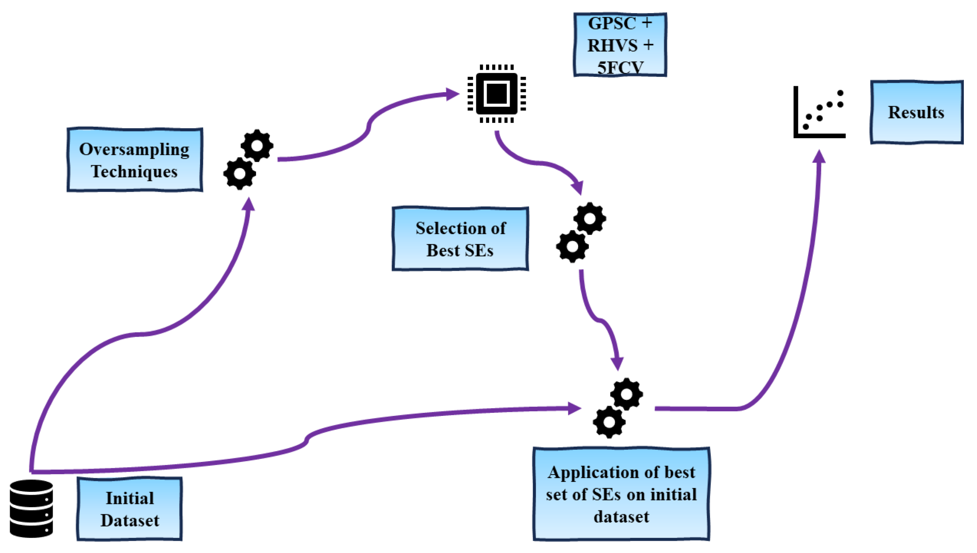
The graphical representation of the research methodology can be observed in Figure 1.
As depicted in Figure 1, the research methodology encompasses the following sequential steps:
- The initial dataset undergoes data processing, involving the transformation of non-numeric type variables into numeric types.
- The preprocessed dataset is subjected to oversampling techniques, including ADASYN, BorderlineSMOTE, KMeansSMOTE, SMOTE, and SVMSMOTE, thereby generating balanced dataset variations.
- Each of the balanced dataset variations is utilized in the Genetic Programming Symbolic Classifier (GPSC) algorithm with the Random Hyperparameter Value Search (RHVS) method during the five-fold cross-validation (5FCV) training process. The RHVS method aims to identify the optimal combination of GPSC hyperparameters, leading to the generation of symbolic expressions (SEs) with high classification accuracy in network intrusion detection.
- The best SEs obtained are combined and assessed on the original imbalanced dataset.
2.2. Dataset Description
In this research, a publicly available dataset from Kaggle [22] has been used. The provided dataset for auditing encompasses a diverse range of simulated intrusions within a military network setting. The dataset was generated to capture raw TCP/IP dump data in a manner simulating a typical US Air Force Local Area Network (LAN). This LAN emulation was meticulously designed to mirror a realistic environment, subjected to multiple simulated attacks. In the context of this simulation, a connection refers to a sequence of TCP packets spanning a specific time duration, during which data traverse between a source IP address and a target IP address following a well-defined protocol. Each connection in the dataset is categorized as either “normal” or identified with a specific attack type. Each connection record is composed of approximately 100 bytes.
For both normal and attack data, a total of 41 features, comprising a mix of quantitative and qualitative attributes (3 qualitative and 38 quantitative features), are extracted for each TCP/IP connection. These features provide a comprehensive representation of the network behavior during these connections. The class variable assigned to each connection holds two distinct categories: “Normal” for regular, non-anomalous connections, and “Anomalous” for those associated with specific attack types. This classification scheme allows for the characterization and analysis of network activities, aiding in the identification and understanding of potential security threats within the simulated military network environment.
The initial problem with the dataset is that some dataset variables are in a non-numeric format, and if they want to be used in the dataset, they have to be transformed into a numeric type. The non-numeric type dataset variables are “protocol-type”, “service”, “flag”, and “class”. The process of transforming the aforementioned variables from a non-numeric to numeric type will be conducted using scikit-learn LabelEncoder function [23]. The results of the LabelEcnoder function applied to non-numeric dataset variables are listed in Table 2.
Unfortunately, the LabelEncoder did not transform the class variable as planned, i.e., to transform the “normal” class label to 0 and the “anomaly” class label to 1, so this was performed manually. However, the result is listed in the Table 2. Additionally from the protocol type variable that was transformed into a numeric type using the OneHotEncoder function from scikit-learn library [23], three new variables were created, i.e., “protocol_type_tcp”, “protocol_type_udp”, and “protocol_type_icmp”. The initial variable “protocol” was removed from the dataset. So the total number of dataset variables was increased from an initial 41 to 44.
After all the non-numeric variables were transformed into numeric variables, the initial statistical analysis was performed. In other words, the dataset was investigated for missing values, and the mean, standard deviation, minimum, and the maximum values were determined for each dataset variable. The results of the initial statistical analysis are listed in Table 3.
From Table 3, it can be noticed based on the “count” value that all dataset variables have the same number of samples, i.e., there are no missing values. All dataset variables have a minimum value equal to 0 with the exception of the “count” and “srv_count” variables, which have a minimum value equal to 1. From the mean, standard deviation, min, and max values, the outliers can be easily detected. Outliers are data points that significantly deviate from the rest of the dataset, often indicating unusual or erroneous observations. Outliers can adversely affect the performance of AI methods by distorting models and leading to biased or inaccurate predictions, as these methods may overly rely on or be disproportionately influenced by the presence of outliers in the training data. Based on the mean, std, and min/max values, the duration, service, flag, src_bytes, dst_bytes, hot, num_compromised, num_root, numf_file_creations, num_file_creations, num_access_files, is_guest_login, count, srv_count, dst_host_count, and dst_host_srv_count. However, other dataset variables have outliers, but their entire range is between 0 and 1, so it is extremely small when compared to the value range of aforementioned variables. It should be noted that two variables, i.e., num_outbound_cmds and is_host_login both are 0 (mean, std, min and max are 0). However, further investigation will be conducted using all the dataset variables and with the outliers intact. The idea is to see if using the initial set of variables the SEs can be obtained for network intrusion detection.
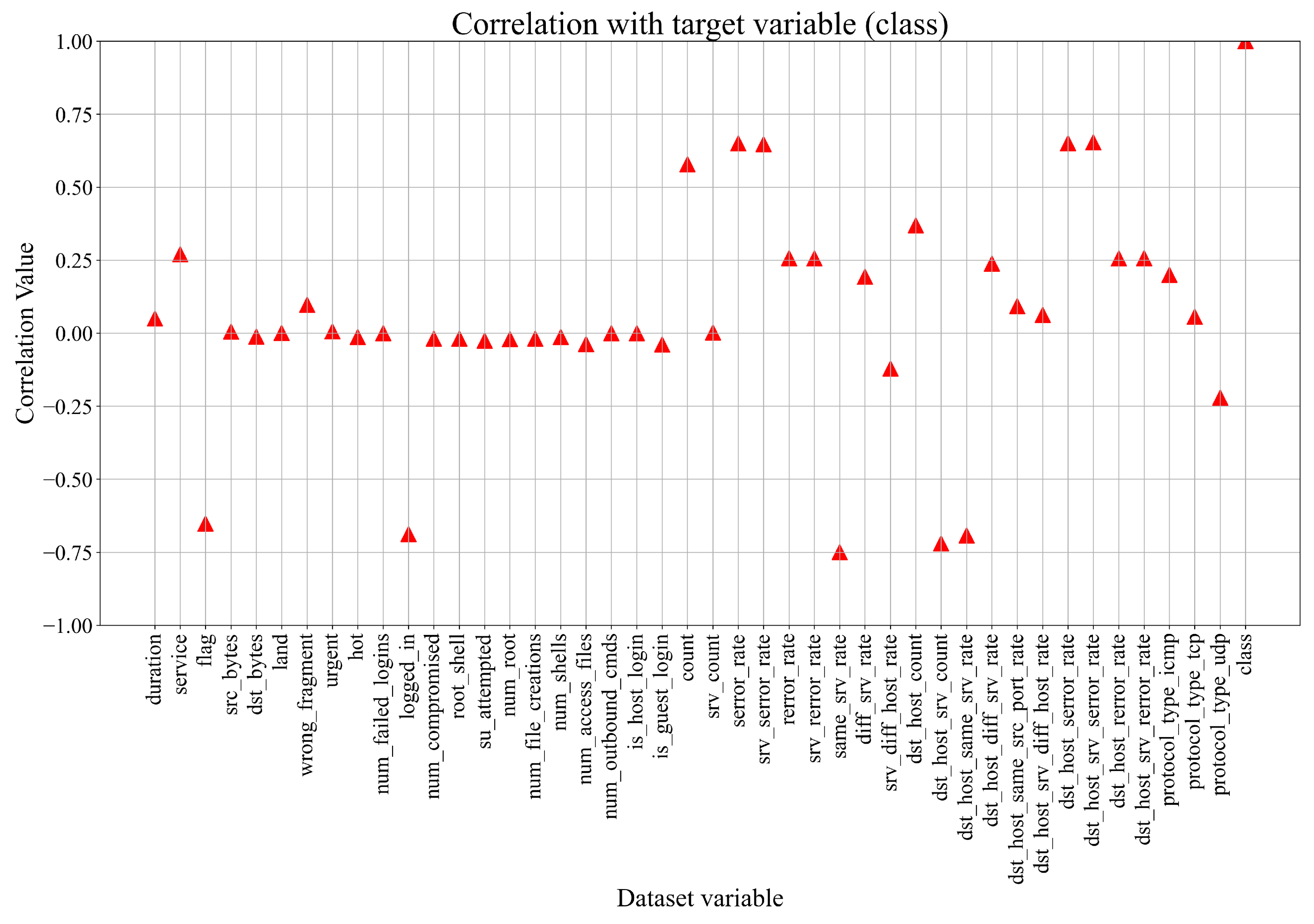
To see the relation between the variables, the correlation analysis must be performed. Here, Pearson’s correlation analysis is used, and the range of correlation value between two variables can be from −1.0 up to 1.0 [24]. The lowest negative value indicates perfect negative correlation, which means that if the value of one variable increases, the value of the other variable will decrease, and vice versa. In the case of the perfect positive correlation between two variables, if the value of one variable increases, the value of the other will also increase. If the correlation value between two variables is 0, it means that both variables do not affect each other. The result of the correlation analysis is shown in Figure 2.
As seen from Figure 2, 19 out of 43 input variables have a correlation of 0 with the class variable, which means that the change in values of these variables will not have any effect on the class variable. The 8 input variables have a correlation value of 0.25 with the class variable. A total of 5 input variables have a positive correlation in the 0.50 to 0.75 range with the class variable, which indicates a strong correlation with the target variable. For reference, the class variable with itself has a perfect correlation of 1. Regarding the negative correlation, two variables (srv_diff_host_rate and protocol_type_udp) have a negative correlation in the −0.12 to −0.25 range with the class variable. The 5 input variables (flag, logged_in, same_srv_rate, dst_host_srv_count, dst_host_same_srv_rate) have negative correlation values in the −0.5 to −0.75 range to the class variable.
Outlier detection plays a crucial role in the field of data analysis and statistical modeling due to its multifaceted impact on various aspects of data interpretation and decision-making. An outlier, defined as a data point significantly differing from the majority, serves as a valuable indicator of potential errors, irregularities, or exceptional cases within a dataset [25]. Detecting outliers is fundamental for maintaining data quality, as they often reveal issues in data collection, measurement processes, or data entry errors. By addressing outliers, analysts can enhance the reliability of datasets, contributing to more accurate and trustworthy analyses.
The influence of outliers on statistical inferences cannot be understated. Outliers possess the ability to unduly impact measures like means and standard deviations, leading to skewed and biased results. Proper outlier detection and management are essential for ensuring that statistical analyses provide a more robust and unbiased representation of the underlying data distribution. Additionally, outliers can negatively affect the performance of predictive models. Machine learning algorithms trained on datasets containing outliers may yield less accurate and skewed predictions. Therefore, the identification and appropriate handling of outliers during data preprocessing is vital for optimizing model performance.
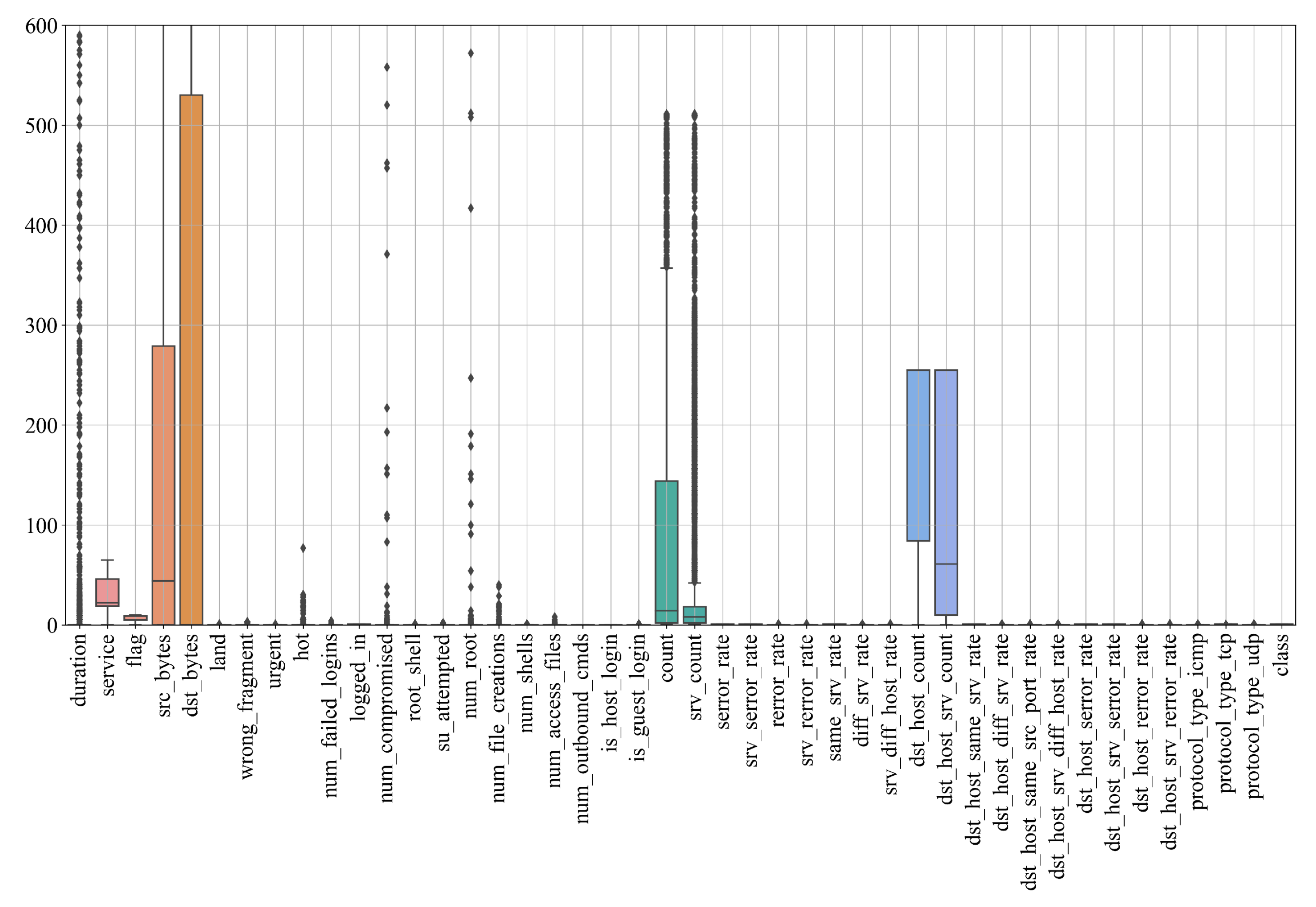
One of the widely employed tools for visualizing data distributions and identifying outliers is the boxplot, also known as the box-and-whisker plot [26]. This graphical representation provides a succinct summary of key statistical measures, including the median, quartiles, and potential outliers. The box encompasses the interquartile range (IQR), representing the span between the first and third quartiles, while the whiskers extend to the minimum and maximum values within a specified range. Outliers, lying outside the whiskers, are typically plotted individually. Boxplots are valuable in data exploration, offering insights into the spread and central tendency of a dataset. Their ability to highlight outliers aids analysts in making informed decisions about data integrity and in developing more accurate and reliable models. The boxplot showing potential outliers is shown in Figure 3.
The value range on the y-axis is limited to 600 since the majority of variables shown in Figure 3 have a range below 600. However, the duration (), src_bytes (), dst_bytes (), num_compromised (), num_root () have max values above 600. From Table 3 and Figure 3, it can be concluded that the dataset contains a large number of dataset variables with outliers. However, the investigation was conducted without handling outliers or applying the dataset scaling and normalization techniques.
From Table 2 and Table 3, it can be noticed that the class variable does not contain an equal number of samples among class labels. The number of class samples is shown in the form of the barplot in Figure 4.
As seen from Figure 4, the normal class has more samples than the anomaly class (11,743). Although the difference between class samples indicates the class imbalance, the difference between class samples is not so large. However, various oversampling techniques will be applied to obtain the balanced dataset variations, which will be used in GPSC to obtain SEs.
2.3. Dataset Oversampling Techniques
The dataset oversampling techniques were used in this research to achieve the balance between class samples. The reason for choosing the oversampling instead of undersampling techniques is because the oversampling techniques do not require any parameter tuning and they are usually faster in reaching the balance between class samples. In this research, the ADASYN, BorderlineSMOTE, KMeansSMOTE, SMOTE, and SVMSMOTE were used.
Adaptive Synthetic Sampling (ADASYN) is an oversampling technique used in ML to address the class imbalance problem [27]. It focuses on generating synthetic examples for the minority class in a dataset by considering the density distribution of different classes. ADASYN adapts its synthetic sample generation based on the density of instances in the feature space, giving more emphasis to regions with fewer instances.
Borderline Synthetic Minority Over-sampling Technique (BorderlineSMOTE) [28] is a variant of the Synthetic Minority Over-sampling Technique (SMOTE) specifically designed to address the issue of class imbalance. It identifies the instances near the decision boundary (borderline instances) between the minority and majority classes and focuses on generating synthetic examples for these instances. This helps improve the classifier’s performance in regions where the decision boundary is more challenging.
KMeansSMOTE is an extension of the SMOTE algorithm that incorporates k-means clustering to generate synthetic samples [29]. It involves clustering the minority class instances using k-means and then applying SMOTE independently within each cluster. This approach aims to capture the underlying structure of the minority class more effectively by generating synthetic samples based on local information.
The Synthetic Minority Over-sampling Technique (SMOTE) is a classic oversampling technique used to address class imbalance in machine learning [30]. It works by generating synthetic examples for the minority class by interpolating between existing instances. Specifically, for each minority class instance, SMOTE selects its k-nearest neighbors and creates synthetic instances along the line segments connecting them. This helps balance the class distribution and improve the classifier’s performance in the minority class.
The Support Vector Machine Synthetic Minority Over-sampling Technique (SVMSMOTE) is an oversampling technique that combines the principles of SMOTE with support vector machines [31]. It aims to generate synthetic samples for the minority class by considering the support vectors obtained from a support vector machine classifier. SVMSMOTE focuses on areas where the decision boundary is more complex and where the support vectors are located, making it particularly useful in capturing the intricacies of the minority class distribution.
The number of samples for each class after the application of the aforementioned techniques is listed in Table 4.
As seen from Table 4, it can be noticed that all the techniques have been successful in balancing the initial dataset. In the case of ADASYN, the minority class (class_1) has 25 fewer samples than the (class_0). In the case of KMeansSMOTE, the minority class (class_1) has 1 more sample than the majority class (class_0). However, these two cases can be considered balanced since in the initial dataset, the minority class (class_1) has 1706 fewer samples than the majority class. In the case of BorderlineSMOTE, SMOTE, and SVMSMOTE, the perfect balance is reached. It should be noted that after the application of these oversampling techniques, balanced dataset variations were created, and a Genetic Programming Symbolic Classifier will be applied to these datasets to obtain SEs.
2.4. Genetic Programming Symbolic Classifier
The Genetic Programming Symbolic Classifier (GPSC) is an evolutionary algorithm that initiates its iterative process by generating random SEs, providing rudimentary estimations of the target variable. Through successive generations, facilitated by genetic operations such as crossover and mutation, GPSC refines these expressions to accurately estimate the target variable. Unlike genetic algorithms, GPSC necessitates a dataset with well-defined input and output variables.
To attain elevated classification accuracy, the meticulous tuning of GPSC hyperparameters is imperative. The optimal combination of hyperparameter values, essential for the derivation of SEs with superior classification accuracy, is achieved through the application of the Random Hyperparameter Value Search (RHVS) method. RHVS, in each invocation, randomly selects hyperparameter values from predefined ranges. The critical GPSC hyperparameters subjected to this search process encompass the following:
- Population size: the size of the SE population undergoing evolution.
- Number of generations: The maximum evolutionary generations and termination criterion. If the minimum fitness function value (stopping criteria value) is not reached during the GPSC execution, the execution will be terminated after a predefined value of the number of generations is reached.
- Tournament size: the size of randomly selected population members competing for parent status.
- Initial tree depth: the depth range of population members represented as tree structures.
- Stopping criteria: The predefined minimum value of the fitness function, a termination criterion. If the value is reached by one of the population members during the GPSC execution, the GPSC execution will be terminated and usually will produce the SEs with good classification accuracy.
- Crossover probability: the likelihood of the crossover genetic operation.
- Subtree mutation probability: the probability of the subtree mutation genetic operation.
- Hoist mutation probability: the probability of the hoist mutation genetic operation.
- Point mutation probability: the probability of the point mutation genetic operation.
- Range of constant values: the predefined range for generating constant values.
- Maximum number of samples: The maximum number of training set samples used for the evaluation of population members. If the value is lower than 1.0, the out-of-bag (OOB) fitness value is calculated. The OOB fitness value is the value obtained when unseen training samples are used in population members in each generation. This is a good metric to see how well population members perform on unseen training data. It is good practice to calculate the OOB to see if the fitness value is near the fitness value of the best population member in each generation. If the value drastically differs from the best fitness value, it could indicate that the obtained SEs, in particular, GPSC, execution will have low classification performance on new data, i.e., overfitting occurs. The best practice is to set this value in the 0.99 to 0.9999 range to ensure that the maximum amount of training data is used for training the population members but also to obtain an OOB fitness value in each generation on a small portion of unseen data samples.
- Range of constant values: This is a hyperparameter that defines the range of constant values that will be used to develop the initial population from a random selection of constant values and also during the mutation operations. The choice of the constant values range is arbitrary.
- Parsimony coefficient: A coefficient mitigating the bloat phenomenon, controlling population growth.
Furthermore, GPSC incorporates mathematical functions, such as addition, subtraction, multiplication, division, natural logarithm, logarithms with bases 2 and 10, square root, cube root, absolute value, sine, cosine, and tangent. Modifications were necessary for certain functions, namely square root, division, natural logarithm, and logarithms with bases two and ten, to avert computational errors. These adjustments are detailed in the Appendix A.1.
To determine the optimal range for each GPSC hyperparameter during RHVS, preliminary testing was conducted, resulting in the delineation of upper and lower boundaries. The comprehensive analysis of these boundary values is presented in Table 5. This meticulous approach ensures the judicious selection of hyperparameter values, thereby enhancing the efficacy of GPSC in achieving heightened classification accuracy on diverse dataset variations.
2.5. Evaluation Metrics
The evaluation metrics used in this research are accuracy (), area under receiver operating characteristics curve (), precision, recall, F1-score, and confusion matrix. The accuracy is a measure of the overall correctness of a classification model [32]. It represents the ratio of correctly predicted instances to the total number of instances. The is calculated using the expression:
where , , , and are true positives (correctly predicted positive instances), true negatives (correctly predicted negative instances), false positives (actual negatives incorrectly predicted as positives), and false negatives (actual positives incorrectly predicted as negatives).
The represents the area under the receiver operating characteristic curve [33]. The ROC curve is a graphical representation of the trade-off between sensitivity (true positive rate) and specificity (true negative rate) for different threshold values. The value is between 0 and 1, with a higher value indicating a better-performing model. It is often calculated using integral calculus on the ROC curve.
The precision is the ratio of correctly predicted positive instances to the total predicted positive instances [34]. It assesses the accuracy of positive predictions. The precision is calculated using the expression, which can be written as:
The recall measures the ratio of correctly predicted positive instances to the total actual positive instances [34]. It assesses the ability of the model to capture all positive instances. Recall is calculated using the expression:
The F1-score is the harmonic mean of precision and recall [34]. In other words, it provides a balance between precision and recall. The F1-score is calculated using the expression:
A confusion matrix is a fundamental tool in the evaluation of the performance of a classification model. It is a table that summarizes the predictions made by a model on a set of data for a binary or multiclass classification problem. The matrix provides a clear and detailed breakdown of the model’s performance, categorizing predictions into four possible outcomes: true positives (TPs), true negatives (TNs), false positives (FPs), and false negatives (FNs). The confusion matrix form is shown in Table 6.
By examining the values in the confusion matrix, one can derive various performance metrics such as accuracy, precision, recall, and the F1-score. These metrics provide insights into different aspects of the model’s effectiveness, such as its ability to correctly classify positive and negative instances, its precision in positive predictions, and its recall or sensitivity in capturing positive instances.
The confusion matrix is an invaluable tool for assessing the strengths and weaknesses of a classification model, helping practitioners make informed decisions about model adjustments and improvements based on specific business or application requirements.
2.6. Training/Testing Procedure
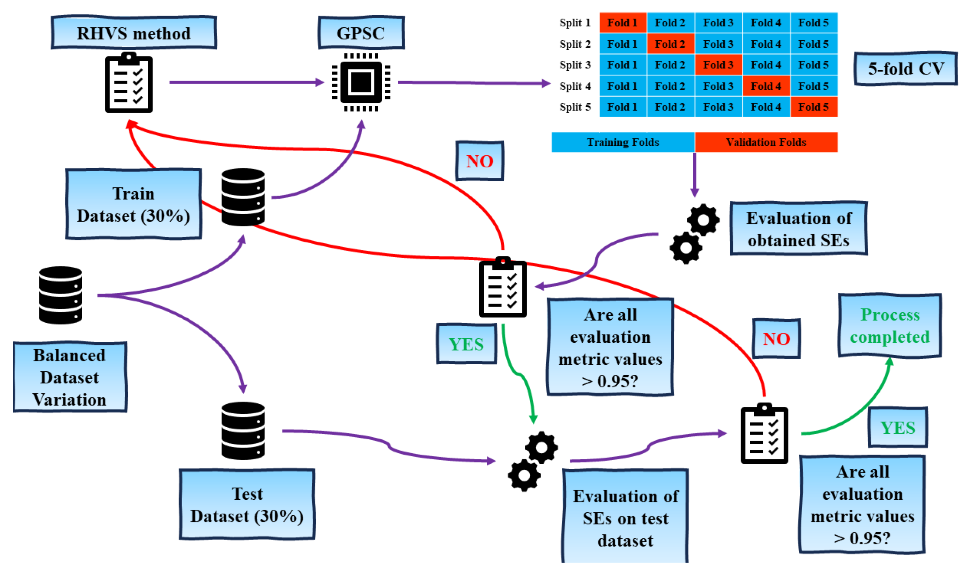
The training and testing procedure is graphically shown in Figure 5.
As illustrated in Figure 5, the training–testing procedure unfolds through a sequence of meticulously orchestrated steps:
- Initial Dataset Division: The balanced dataset variation is initially partitioned into training and testing sets at a ratio of 70:30.
- Training Phase: The training dataset serves as input to the GPSC algorithm within a 5-fold cross-validation framework. Prior to the execution of GPSC, its hyperparameter values undergo a random selection process from predefined ranges facilitated by the RHVS method.
- Evaluation Metrics Calculation: Following the completion of 5-fold cross validation, the mean and standard deviation values for evaluation metrics (, , precision, recall, and F1-score) are computed based on the outcomes from the five trained models (SEs). If the mean values for all evaluation metrics surpass 0.95, the process advances to the testing phase. Otherwise, the algorithm iterates, initiating a new cycle by randomly selecting hyperparameter values.
- Testing Phase: In this phase, the SEs derived from the training process are evaluated on the designated testing dataset. Subsequently, the mean values for the evaluation metrics are computed. If these values exceed 0.95 across all metrics, signifying a high level of performance, the process concludes. If not, the iteration resumes, commencing afresh with the random selection of hyperparameter values. This cyclic procedure ensures a rigorous and iterative approach, striving for optimal SEs that meet the defined performance criteria.
3. Results
Within this section, the outcomes showcase the optimal SEs derived from the balanced dataset variations. Subsequently, these premier SEs were amalgamated into an ensemble and subjected to testing on the initial imbalanced dataset. The ensuing examination delves into the classification performance of the ensemble, considering the tally of accurate predictions as a pivotal metric.
3.1. The Best Symbolic Expressions
The premier SEs acquired from each balanced dataset variation were derived through the selection of optimal GPSC hyperparameter values, determined randomly via the RHVS method. The particulars of the optimal GPSC hyperparameter values, instrumental in obtaining the most effective SEs for each balanced dataset variation, are enumerated in Table 7.
Examining Table 7 reveals distinctive trends in the selection of optimal GPSC hyperparameter values across various balanced dataset variations. Notably, the SVMSMOTE dataset application necessitated the utilization of the highest population size, followed closely by the ADASYN dataset. In contrast, the remaining datasets saw GPSC employ lower population size values, strategically aligned near the lower boundary of the Random Hyperparameter Value Search (RHVS) method as delineated in Table 5. The adoption of a larger population size assumes significance in fostering heightened diversity within the population.
Crucially, an additional pivotal hyperparameter influencing population diversity is the initial tree depth. The SMOTE dataset witnessed the implementation of the most substantial initial tree depth, whereas the ADASYN dataset observed the application of the smallest depth. The predominant termination criterion for GPSC in this investigation was the number of generations. Given the dual termination criteria within GPSC—number of generations and stopping criteria—the latter remained unmet throughout, as its predetermined value (minimum fitness function value) proved exceptionally low, preventing attainment by any population member. The stopping criteria ranged from for the SMOTE dataset to for the SVMSMOTE dataset.
A prevailing genetic operation in this study was the subtree mutation, consistently featuring values of 0.95 or higher. The max samples parameter consistently exceeded 0.99 across all GPSC executions. Notably, the KMeansSMOTE dataset exhibited the broadest range of constant values (−735.19, 492.48), signifying a distinctive range of evolutionary operations. Examining the parsimony coefficient values from Table 7, it is evident that the coefficients are uniformly diminutive, with the KMeansSMOTE dataset registering the lowest () and the BorderlineSMOTE dataset recording the highest () coefficient. Despite their modest values, these parsimony coefficients effectively mitigated the bloat phenomenon, ensuring the stability and efficiency of GPSC executions in this investigation.
In Figure 6, the change of loss value (fitness function value) over number of generations for one split in 5FCV is shown in case of GPSC and MLP Classifier applied on the SMOTE dataset. The MLP Classifier configuration consisted of three hidden layers with relu activation function. The first hidden layer consisted of 50 neurons; the second, 20 neurons; and third, 10 neurons. The MLP Classifier was just used for comparison and is labeled ANN in Figure 6.
As seen from Figure 6, the log-loss value in the first 50 generations drops from 0.5 to 0.08 value and continuously decreases up to the 248th generation. However, the drop from the 50th to 248th generation is much lower when compared to the drop in the first 50 generations. On the other hand, ANN (MLP classifier) showed a high drop in value in the first 20 iterations, and up to the 248th iteration, the decrease in the loss function was low. When these loss values are compared, it can be noticed that the GPSC outperformed the ANN.
The evaluation metric values of the best SEs obtained on the train and test datasets are graphically shown in Figure 7.
Examining Figure 7 reveals notable disparities in the classification performance of the best SEs derived from diverse balanced dataset variations. Particularly, the highest classification performance is discerned in SEs obtained from the SVMSMOTE dataset. A descending order of classification performance follows for SEs derived from SMOTE, KMeansSMOTE, BorderlineSMOTE, and ADASYN datasets. It is noteworthy that even the SEs obtained from the ADASYN dataset exhibit commendable classification accuracy, albeit the lowest in this comparative analysis, standing at 0.968.
Across all balanced dataset variations, the standard deviation for the best SEs is remarkably small, underscoring the consistency of performance. The set of SEs derived from the BorderlineSMOTE dataset, specifically in terms of mean precision, yields the lowest standard deviation. Notably, when comparing the standard deviation among the best SEs obtained from diverse dataset variations for all evaluation metrics, a slightly elevated standard deviation is observed in the case of SEs derived from the ADASYN dataset.
As elucidated in the GPSC description, the size of obtained SEs can be assessed through two dimensions: depth and length. Depth is measured along the tree structure representation during GPSC execution, spanning from the root node (the first element in text representation) to the deepest leaf. Length, on the other hand, quantifies the entirety of elements within a symbolic expression, encompassing mathematical functions, input variables, and constants.
For a comprehensive understanding, Table 8 enumerates the depth and length measurements for the best SEs acquired from diverse balanced dataset variations.
Analyzing Table 8 reveals distinctive characteristics in the depth and length metrics of SEs obtained from various balanced dataset variations. Notably, SEs acquired from the BorderlineSMOTE dataset exhibit the lowest average depth and length, while those derived from the KMeansSMOTE dataset showcase the highest average values for both depth and length. The SEs obtained from the SVMSMOTE dataset, conversely, demonstrate the highest average length.
Further scrutiny of Table 8 underscores that SEs sharing identical depth values may exhibit dissimilar lengths. For instance, SE1 and SE2 obtained from the BorderlineSMOTE dataset both possess a depth of 16, yet SE1 has a length of 92, while SE2 spans 114 elements. A similar trend is observed for SE4 obtained from the KMeansSMOTE dataset, where despite an equal depth of 17, the length registers as 129.
This decoupling of depth and length is further exemplified by SE5 from the ADASYN and KMeansSMOTE datasets, as well as SE2 from the SVMSMOTE dataset, all featuring a shared depth of 17, yet showcasing distinct length values: 160, 177, and 123, respectively. These instances illustrate that identical depth values do not imply uniform length values for SEs.
Subsequent analysis of the best SEs illuminates the requisite input variables for their utilization. With the exception of , , , , and , the majority of input variables are essential for incorporating all the best SEs. Distinct sets of non-essential variables emerge for SEs obtained from different dataset variations. For instance, the best SEs from the ADASYN dataset do not necessitate , , , , , , and . In comparison, the best SEs from the BorderlineSMOTE dataset, in addition to the aforementioned variables, also exclude , , and . Analogously, the best SEs from the KMeansSMOTE dataset exclude , , and , while those from the SMOTE dataset omit , , , , , and . Finally, the best SEs from the SVMSMOTE dataset, apart from , , , , and , do not require .
For a detailed guide on downloading and utilizing the obtained SEs, refer to Appendix A.2.
3.2. Evaluation on the Original Dataset
In the previous subsection, we presented the results of the 25 best SEs, which are obtained on three balanced dataset variations. To final evaluation will be performed by applying the 25 best SEs on the original imbalanced dataset. The evaluation process of each symbolic expression consists of the following steps:
- Uses input variables from the original dataset in symbolic expression to compute the output;
- Uses this output in the sigmoid function to determine the class (0 or 1).
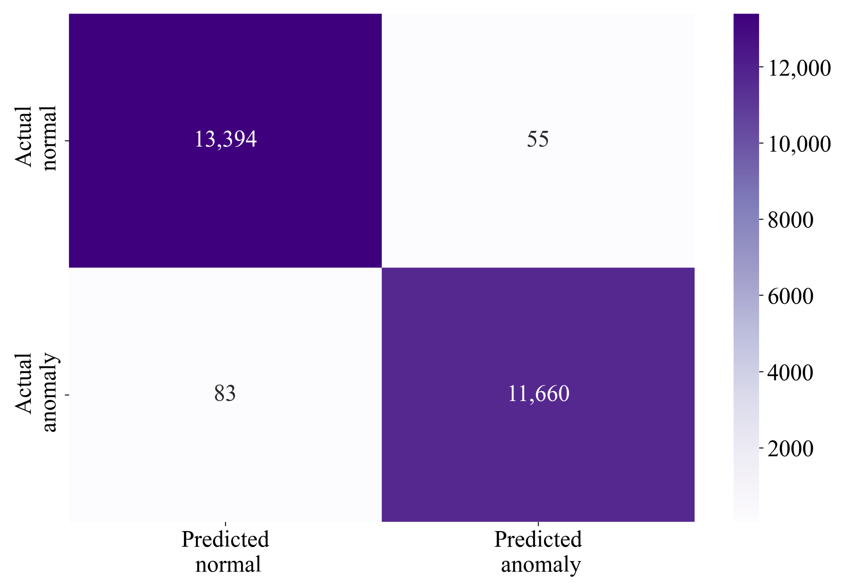
The highest classification performance was achieved if at least 15 SEs had an accurate prediction per dataset sample. The classification performance of the 25 best SEs is shown in Table 9 and Figure 8.
The evaluation metric values obtained by application of the best set of all SEs on the initial imbalanced dataset showed high classification performance.
The confusion matrix shown in Figure 8 confirms the accuracy shown in Table 9. If the TP, TN, FP, and FN values are used from the confusion matrix and used in the equation, the value of 0.9938 would be obtained. The confusion matrix indicates that only 41 normal samples were misclassified out of 13,449 in total, which is 0.3%. In the case of anomaly, only 115 samples were misclassified out of 11,743 in total, which is 0.9%.
4. Discussion
In this investigation, the utilization of a publicly available dataset was instrumental in the derivation of SEs employing the GPSC for the purpose of network intrusion detection, with a specific focus on achieving elevated classification performance. The initial dataset, characterized by its imbalanced nature, necessitated meticulous data preprocessing, particularly in transforming variables from a string to numeric format. The outcomes of these transformations are meticulously detailed in Table 2.
Subsequent to the application of the LabelEncoder for dataset transformation, an initial statistical analysis was conducted to ascertain crucial parameters, such as minimum, maximum, mean, and standard deviation. This analysis revealed a dataset void of missing values, comprising 25,192 samples across all 44 variables, including the output (target) variable. However, two variables, namely num_outbound_cmds and is_host_login, exhibited constant values of 0. Despite this, these values were retained within the dataset. The statistical summary exposed a uniform minimum value of 0 across all dataset variables. The class variable demonstrated a mean value of 0.53 and a standard deviation of 0.49, indicative of a marginal class imbalance, necessitating potential oversampling.
Given the substantial number of variables, the exploration of a correlation matrix proved inelegant for this study. Consequently, Pearson’s correlation analysis focused solely on the class variable, revealing noteworthy insights portrayed in Figure 2. This analysis unveiled that merely five input variables exhibited a positive correlation with the class variable, while another five displayed a robust negative correlation. Notably, a majority of variables exhibited correlations below 0.5 or above −0.5, suggesting proximity to zero.
Efforts were directed towards balancing the initially imbalanced dataset through the application of the BorderlineSMOTE, SMOTE, and SVMSMOTE oversampling techniques. However, perfect balance was not universally achieved as evidenced by ADASYN and KMeansSMOTE. Despite a marginal discrepancy in the sample counts, the dataset variations obtained using ADASYN and KMeansSMOTE were considered well balanced and were consequently employed in this investigation.
The implementation of GPSC, coupled with a Random Hyperparameter Value Search method on each dataset variation, demanded time investments to ascertain the optimal hyperparameter values conducive to the derivation of SEs boasting optimal classification performance. The examination of optimal hyperparameter combinations revealed nuanced patterns, such as varying population sizes and termination criteria across different oversampled datasets.
The culmination of this research is embodied in the performance evaluation of the best SEs on balanced dataset variations (Figure 7). The achieved classification performance exhibited a remarkable range of accuracy, consistently surpassing 0.96 and falling below 0.985. The subsequent application of the amalgamated best SEs to the initial imbalanced dataset yielded exceptional evaluation metric values, each exceeding 0.99 (Table 8). The confusion matrix (Figure 8) attested to the superb performance of the best SEs, with minimal misclassifications observed.
A comparative analysis of the proposed approach and results vis à vis prior research is elucidated in Table 10, underscoring the noteworthy contributions of the presented methodology.
Upon scrutinizing the results comparison delineated in Table 9, it becomes evident that the research proposed in this paper exhibits superior performance in contrast to a majority of outcomes reported in other research papers. While acknowledging that the results in [12] marginally surpass those presented herein, it is noteworthy that the proposed methodology outperforms a significant array of alternative investigations.
The distinctive advantage conferred by the presented methodology in this paper lies in the acquisition of SEs capable of network intrusion detection with exceptional classification accuracy. The SEs, once obtained, offer the distinct benefit of efficient storage and obviate the need for substantial computational resources when calculating outputs for new samples. This attribute further underscores the practicality and efficiency of the proposed approach.
5. Conclusions
In this study, the utilization of a publicly available dataset within the GPSC framework aimed at obtaining SEs for network intrusion detection demonstrated remarkable outcomes in terms of high classification performance. The initial challenge posed by class imbalance in the dataset was addressed through meticulous preprocessing, including the application of a Label Encoder to transform string values into numeric representations. Subsequently, oversampling techniques, namely, ADASYN, BorderlineSMOTE, KMeansSMOTE, SMOTE, and SVMSMOTE, were employed to generate balanced dataset variations. These balanced datasets served as the basis for GPSC training via a five-fold cross-validation (5FCV) procedure, facilitated by the development and application of the Random Hyperparameter Value Search (RHVS) method. The RHVS method effectively identified optimal GPSC hyperparameter values crucial for achieving SEs with the highest classification accuracy. The aggregation of the best SEs from each balanced dataset variation, when applied to the initial preprocessed imbalanced dataset, aimed to ascertain if comparable estimation accuracy levels could be sustained. The key conclusions drawn from this investigation include the following:
- The investigation showed that by using GPSC, SEs with high classification performance can be obtained. Using the five-fold cross-validation process proved to be useful since GPSC on each split generated a symbolic expression which added to the robustness of the trained model.
- The application of oversampling techniques was successful, and using them, the balanced dataset variations were created. On these datasets, the GPSC generated the SEs with very high classification performance. So, it can be concluded that the oversampling techniques had a great influence on classification performance, and, using different balancing techniques, multiple SEs were obtained, adding to the robustness of the final SE ensemble.
- The application of the RHVS method proved to be very useful in searching for the optimal combination of hyperparameters. On each balanced dataset variation, the method found the optimal combination of GPSC hyperparameters, with which the highest classification performance of the obtained SEs was achieved.
- Combining the best SEs into an ensemble added to the robustness in the network intrusion detection. The investigation showed that at least 60% (15 out of 25 SEs) of SEs have to have correct prediction in order to achieve the highest classification performance.
Advantages of the proposed methodologies encompass the following:
- The capacity of GPSC to yield SEs with elevated classification accuracy: these SEs, distinctively simplistic in comparison to Artificial Neural Networks (ANNs) or Convolutional Neural Networks (CNNs), lend themselves to facile storage and processing, demanding minimal computational resources.
- The efficacy of the RHVS method in identifying optimal GPSC hyperparameter values, contributing to the efficiency of the entire process.
- The reliability of the 5FCV procedure in producing a resilient ensemble of highly accurate SEs.
However, certain limitations are acknowledged:
- The combination of number of generations and stopping criteria greatly prolonged the execution of the GPSC. Since the stopping criteria value (predefined minimum fitness function value) was so low, it was not reached by any population member in all GPSC executions conducted in this research, so each GPSC execution was determined after a predefined maximum number of generations was reached.
- Although the combination of GPSC with RHVS and trained using five-fold cross validation is a good procedure to find the optimal combination of hyperparameter values, with which GPSC will generate five SEs with high classification accuracy, the process can take a long time since for each combination of randomly selected hyperparameter values, the GPSC has to be repeated five times (due to the 5FCV training procedure) and finally evaluated to obtain the classification performance metric values. If these values are above 0.95, then the process is terminated.
The future work will be focused on multiple network intrusion datasets to see if the same SEs with highest classification performance obtained on one dataset can be applied to other datasets as well. The ranges used in the RHVS method will be investigated in future work to see if the same or even better classification performance can be achieved using a smaller population and number of generations. In future work, the response time in the network intrusion detection of obtained SEs and other ML algorithms will be compared. Although the RHVS method proved useful in finding the optimal combination of GPSC hyperparameters, in future work, the other optimization algorithms, such as genetic algorithm, particle swarm optimization, and others, will be investigated to determine if they can find the optimal combination of hyperparameters faster.These future research directions aim to refine and extend the proposed methodology, providing valuable insights into the intricacies of network intrusion detection and the optimization of symbolic expression generation.
Author Contributions
Conceptualization, N.A. and S.B.Š.; methodology, N.A. and S.B.Š.; software, N.A. and S.B.Š.; validation, N.A. and S.B.Š.; formal analysis, N.A. and S.B.Š.; investigation, N.A. and S.B.Š.; resources, N.A. and S.B.Š.; data curation, N.A. and S.B.Š.; writing—original draft preparation, N.A. and S.B.Š.; writing—review and editing, N.A. and S.B.Š.; visualization, N.A. and S.B.Š.; supervision, N.A.; project administration, N.A.; funding acquisition, N.A. All authors have read and agreed to the published version of the manuscript.
Funding
This research was (partly) supported by the CEEPUS network CIII-HR-0108, the European Regional Development Fund under Grant KK.01.1.1.01.0009 (DATACROSS), the Erasmus+ project WICT under Grant 2021-1-HR01-KA220-HED-000031177, and the University of Rijeka Scientific Grants uniri-mladi-technic-22-61 and uniri-tehnic-18-275-1447.
Institutional Review Board Statement
Not applicable.
Informed Consent Statement
Not applicable.
Data Availability Statement
Dataset is available at https://www.kaggle.com/datasets/sampadab17/network-intrusion-detection accessed on 10 December 2023.
Conflicts of Interest
The authors declare no conflicts of interest.
Appendix A
Appendix A.1. Modification of Mathematical Functions Used in GPSC
As stated in the description of GPSC, some mathematical functions, i.e., division, square root, natural log, and log with bases 2 and 10, had to be modified to avoid ill GPSC execution. The division function:
where and are arbitrary variables and do not have any connection with dataset input variables. The square root function was defined as:
The natural log and log with bases 2 and 10 were defined as:
Appendix A.2. Procedure of Using the Obtained SEs
The obtained symbolic expression in this research using GPSC are available at GITHUB repository (https://github.com/nandelic2022/Network-Intrusion-Detection-Initial), accessed on 15 January 2024. After downloading the symbolic expression, download the dataset from Kaggle or use your own. However, when using your own dataset, be sure to check the Materials and Methods section of this paper to see the number of input variables and what these input variables are. When the dataset is prepared and the SEs are ready, the procedure for obtaining results can be summarized as follows:
- Use input dataset variables in each symbolic expression to compute the output;
- Use each output of the symbolic expression as input to the sigmoid function, defined in the description of GPSC algorithm to determine the class (network intrusion detection or not);
- Use the obtained output and real dataset output to compute the evaluation metrics, i.e., determine the classification performance of the SEs.
References
- Patel, A.; Qassim, Q.; Wills, C. A survey of intrusion detection and prevention systems. Inf. Manag. Comput. Secur. 2010, 18, 277–290. [Google Scholar] [CrossRef]
- Aslan, Ö.; Aktuğ, S.S.; Ozkan-Okay, M.; Yilmaz, A.A.; Akin, E. A comprehensive review of cyber security vulnerabilities, threats, attacks, and solutions. Electronics 2023, 12, 1333. [Google Scholar] [CrossRef]
- Thakare, S.; Ingle, P.; Meshram, B. IDS: Intrusion detection system the survey of information security. Int. J. Emerg. Technol. Adv. Eng. 2012, 2, 86–90. [Google Scholar]
- Ghorbani, A.A.; Lu, W.; Tavallaee, M. Network Intrusion Detection and Prevention: Concepts and Techniques; Springer Science & Business Media: Berlin, Germany, 2009; Volume 47. [Google Scholar]
- Li, H.; Yoo, S.; Kettinger, W.J. The roles of IT strategies and security investments in reducing organizational security breaches. J. Manag. Inf. Syst. 2021, 38, 222–245. [Google Scholar] [CrossRef]
- Anwar, S.; Mohamad Zain, J.; Zolkipli, M.F.; Inayat, Z.; Khan, S.; Anthony, B.; Chang, V. From intrusion detection to an intrusion response system: Fundamentals, requirements, and future directions. Algorithms 2017, 10, 39. [Google Scholar] [CrossRef]
- Ismail, W.B.W.; Yusof, M. Mitigation strategies for unintentional insider threats on information leaks. Int. J. Secur. Its Appl. 2018, 12, 37–46. [Google Scholar] [CrossRef]
- Sangkatsanee, P.; Wattanapongsakorn, N.; Charnsripinyo, C. Practical real-time intrusion detection using machine learning approaches. Comput. Commun. 2011, 34, 2227–2235. [Google Scholar] [CrossRef]
- Shenfield, A.; Day, D.; Ayesh, A. Intelligent intrusion detection systems using artificial neural networks. ICT Express 2018, 4, 95–99. [Google Scholar] [CrossRef]
- Ashiku, L.; Dagli, C. Network intrusion detection system using deep learning. Procedia Comput. Sci. 2021, 185, 239–247. [Google Scholar] [CrossRef]
- Al-Yaseen, W.L.; Othman, Z.A.; Nazri, M.Z.A. Multi-level hybrid support vector machine and extreme learning machine based on modified K-means for intrusion detection system. Expert Syst. Appl. 2017, 67, 296–303. [Google Scholar] [CrossRef]
- Gautam, R.K.S.; Doegar, E.A. An ensemble approach for intrusion detection system using machine learning algorithms. In Proceedings of the 2018 8th International Conference on Cloud Computing, Data Science & Engineering (Confluence), Noida, India, 11–12 January 2018; IEEE: New York, NY, USA, 2018; pp. 14–15. [Google Scholar]
- Marir, N.; Wang, H.; Feng, G.; Li, B.; Jia, M. Distributed abnormal behavior detection approach based on deep belief network and ensemble SVM using spark. IEEE Access 2018, 6, 59657–59671. [Google Scholar] [CrossRef]
- Xiao, Y.; Xing, C.; Zhang, T.; Zhao, Z. An intrusion detection model based on feature reduction and convolutional neural networks. IEEE Access 2019, 7, 42210–42219. [Google Scholar] [CrossRef]
- Yin, C.; Zhu, Y.; Fei, J.; He, X. A deep learning approach for intrusion detection using recurrent neural networks. IEEE Access 2017, 5, 21954–21961. [Google Scholar] [CrossRef]
- Shen, Y.; Zheng, K.; Wu, C.; Zhang, M.; Niu, X.; Yang, Y. An ensemble method based on selection using bat algorithm for intrusion detection. Comput. J. 2018, 61, 526–538. [Google Scholar] [CrossRef]
- Shone, N.; Ngoc, T.N.; Phai, V.D.; Shi, Q. A deep learning approach to network intrusion detection. IEEE Trans. Emerg. Top. Comput. Intell. 2018, 2, 41–50. [Google Scholar] [CrossRef]
- Jia, Y.; Wang, M.; Wang, Y. Network intrusion detection algorithm based on deep neural network. IET Inf. Secur. 2019, 13, 48–53. [Google Scholar] [CrossRef]
- Wang, Z. Deep learning-based intrusion detection with adversaries. IEEE Access 2018, 6, 38367–38384. [Google Scholar] [CrossRef]
- Iranmanesh, S.; Abkenar, F.S.; Jamalipour, A.; Raad, R. A Heuristic Distributed Scheme to Detect Falsification of Mobility Patterns in Internet of Vehicles. IEEE Internet Things J. 2022, 9, 719–727. [Google Scholar] [CrossRef]
- Alavizadeh, H.; Alavizadeh, H.; Jang-Jaccard, J. Deep Q-learning based reinforcement learning approach for network intrusion detection. Computers 2022, 11, 41. [Google Scholar] [CrossRef]
- Bhosale, S. Network Intrusion Detection Dataset. 2018. Available online: https://www.kaggle.com/datasets/sampadab17/network-intrusion-detection (accessed on 6 March 2024).
- Pedregosa, F.; Varoquaux, G.; Gramfort, A.; Michel, V.; Thirion, B.; Grisel, O.; Blondel, M.; Prettenhofer, P.; Weiss, R.; Dubourg, V.; et al. Scikit-learn: Machine Learning in Python. J. Mach. Learn. Res. 2011, 12, 2825–2830. [Google Scholar]
- Sedgwick, P. Pearson’s correlation coefficient. BMJ 2012, 345, e4483. [Google Scholar] [CrossRef]
- Osborne, J.W.; Overbay, A. The power of outliers (and why researchers should always check for them). Pract. Assess. Res. Eval. 2019, 9, 6. [Google Scholar]
- Jajo, N.K.; Matawie, K.M. Outlier detection using modified boxplot. Int. J. Ecol. Dev. 2009, 33, 116–122. [Google Scholar]
- He, H.; Bai, Y.; Garcia, E.A.; Li, S. ADASYN: Adaptive synthetic sampling approach for imbalanced learning. In Proceedings of the 2008 IEEE International Joint Conference on Neural Networks (IEEE World Congress on Computational Intelligence), Hong Kong, China, 1–8 June 2018; IEEE: New York, NY, USA, 2008; pp. 1322–1328. [Google Scholar]
- Han, H.; Wang, W.Y.; Mao, B.H. Borderline-SMOTE: A new over-sampling method in imbalanced data sets learning. In Proceedings of the International Conference on Intelligent Computing, Hefei, China, 23–26 August 2005; Springer: Berlin/Heidelberg, Germany, 2005; pp. 878–887. [Google Scholar]
- Douzas, G.; Bacao, F.; Last, F. Improving imbalanced learning through a heuristic oversampling method based on k-means and SMOTE. Inf. Sci. 2018, 465, 1–20. [Google Scholar] [CrossRef]
- Fernández, A.; Garcia, S.; Herrera, F.; Chawla, N.V. SMOTE for learning from imbalanced data: Progress and challenges, marking the 15-year anniversary. J. Artif. Intell. Res. 2018, 61, 863–905. [Google Scholar] [CrossRef]
- Bagui, S.S.; Mink, D.; Bagui, S.C.; Subramaniam, S. Determining Resampling Ratios Using BSMOTE and SVM-SMOTE for Identifying Rare Attacks in Imbalanced Cybersecurity Data. Computers 2023, 12, 204. [Google Scholar] [CrossRef]
- Sokolova, M.; Japkowicz, N.; Szpakowicz, S. Beyond accuracy, F-score and ROC: A family of discriminant measures for performance evaluation. In Proceedings of the Australasian Joint Conference on Artificial Intelligence, Hobart, Australia, 4–8 December 2008; Springer: Berlin/Heidelberg, Germany, 2006; pp. 1015–1021. [Google Scholar]
- de Hond, A.A.; Steyerberg, E.W.; van Calster, B. Interpreting area under the receiver operating characteristic curve. Lancet Digit. Health 2022, 4, e853–e855. [Google Scholar] [CrossRef]
- Goutte, C.; Gaussier, E. A probabilistic interpretation of precision, recall and F-score, with implication for evaluation. In Proceedings of the European Conference on Information Retrieval, Santiago de Compostela, Spain, 21–23 March 2005; Springer: Berlin/Heidelberg, Germany, 2005; pp. 345–359. [Google Scholar]
Figure 1.
The graphical representation of the research methodology.

Figure 2.
The correlation analysis.

Figure 3.
The boxplot shows the variable distribution and possible outliers.

Figure 4.
The number of class samples.

Figure 5.
The graphical representation of training–testing procedure.

Figure 6.
The change of log-los values versus number of generations in the case of GPSC applied to the SMOTE dataset.
Figure 6.
The change of log-los values versus number of generations in the case of GPSC applied to the SMOTE dataset.

Figure 7.
The classification performance of the best sets of SEs obtained on balanced dataset variations.
Figure 7.
The classification performance of the best sets of SEs obtained on balanced dataset variations.

Figure 8.
The confusion matrix of network intrusion detection.


Table 1.
The results reported in other literature.
| References | AI Methods | Results |
|---|---|---|
| [9] | ANN | |
| [10] | CNN | |
| [11] | SVC, ELM | |
| [12] | ensemble method (Naive Bayes, PART and Adaptive Boost) | |
| [13] | multi-layer ensemble method SVC | |
| [14] | CNN | |
| [15] | RNN | |
| [16] | Ensemble based on selection using Bat algorithm | |
| [17] | Non symmetric deep auto encoder with RFC | |
| [18] | DNN | |
| [19] | DNN | |
| [21] | deep Q-learning |
Table 2.
The values of non-numeric variables and their corresponding numeric value after application of the Label encoder. (Beside each variable value is the total number of samples that contain this variable value).
Table 2.
The values of non-numeric variables and their corresponding numeric value after application of the Label encoder. (Beside each variable value is the total number of samples that contain this variable value).
| Variable Name | Value Type | Value |
|---|---|---|
| protocol type | Original Value | ‘tcp’: 20,526, ‘udp’: 3011, ‘icmp’: 1655 |
| Numeric Value | 1: 20,526, 2: 3011, 0: 1655 | |
| service | Original Value | ‘http’: 8003, ‘private’: 4351, ‘domain_u’: 1820, ‘smtp’: 1449, ‘ftp_data’: 1396, ‘eco_i’: 909, ‘other’: 858, ‘ecr_i’: 613, ‘telnet’: 483, ‘finger’: 366, ‘ftp’: 345, ‘auth’: 189, ‘Z39_50’: 172, ‘courier’: 164, ‘uucp’: 157, ‘time’: 155, ‘bgp’: 146, ‘whois’: 145, ‘imap4’: 138, ‘uucp_path’: 133, ‘iso_tsap’: 131, ‘ctf’: 127, ‘urp_i’: 124, ‘nnsp’: 123, ‘supdup’: 114, ‘http_443’: 113, ‘csnet_ns’: 111, ‘efs’: 110, ‘domain’: 109, ‘gopher’: 109, ‘vmnet’: 107, ‘daytime’: 107, ‘discard’: 105, ‘hostnames’: 96, ‘name’: 92, ‘klogin’: 92, ‘exec’: 91, ‘mtp’: 90, ‘ldap’: 90, ‘systat’: 88, ‘netbios_dgm’: 85, ‘link’: 85, ‘login’: 79, ‘netstat’: 78, ‘netbios_ns’: 76, ‘sunrpc’: 67, ‘kshell’: 67, ‘netbios_ssn’: 67, ‘echo’: 65, ‘nntp’: 61, ‘ssh’: 58, ‘pop_3’: 53, ‘sql_net’: 46, ‘IRC’: 40, ‘ntp_u’: 32, ‘X11’: 22, ‘rje’: 20, ‘remote_job’: 17, ‘pop_2’: 17, ‘printer’: 12, ‘shell’: 11, ‘urh_i’: 4, ‘pm_dump’: 3, ‘red_i’: 3, ‘tim_i’: 2, ‘http_8001’: 1 |
| Numeric Value | 22: 8003, 46: 4351, 11: 1820, 51: 1449, 19: 1396, 13: 909, 41: 858, 14: 613, 57: 483, 17: 366, 18: 345, 3: 189, 2: 172, 5: 164, 62: 157, 59: 155, 4: 146, 65: 145, 25: 138, 63: 133, 26: 131, 7: 127, 61: 124, 38: 123, 55: 114, 23: 113, 6: 111, 15: 110, 10: 109, 20: 109, 64: 107, 8: 107, 9: 105, 21: 96, 33: 92, 27: 92, 16: 91, 32: 90, 29: 90, 56: 88, 34: 85, 30: 85, 31: 79, 37: 78, 35: 76, 54: 67, 28: 67, 36: 67, 12: 65, 39: 61, 53: 58, 44: 53, 52: 46, 0: 40, 40: 32, 1: 22, 49: 20, 48: 17, 43: 17, 45: 12, 50: 11, 60: 4, 42: 3, 47: 3, 58: 2, 24: 1 | |
| flag | Original Value | ‘SF’: 14,973, ‘S0’: 7009, ‘REJ’: 2216, ‘RSTR’: 497, ‘RSTO’: 304, ‘S1’: 88, ‘SH’: 43, ‘RSTOS0’: 21, ‘S2’: 21, ‘S3’: 15, ‘OTH’: 5 |
| Numeric Value | 9: 14,973, 5: 7009, 1: 2216, 4: 497, 2: 304, 6: 88, 10: 43, 3: 21, 7: 21, 8: 15, 0: 5 | |
| class | Original Value | ‘normal’: 13,449, ‘anomaly’: 11,743 |
| Numeric Value | 0: 13,449, 1: 11,743 |
Table 3.
The results of the dataset statistical analysis and GPSC variable representation of dataset variables.
Table 3.
The results of the dataset statistical analysis and GPSC variable representation of dataset variables.
| Variable Name | Count | Mean | Std | Min | Max | GPSC Variable Representation |
|---|---|---|---|---|---|---|
| duration | 25,192 | 305.05 | 2686.56 | 0 | 42,862 | |
| service | 29.04 | 15.56 | 65 | |||
| flag | 6.98 | 2.68 | 10 | |||
| src_bytes | 24,330.63 | 2,410,805.40 | ||||
| dst_bytes | 3491.85 | 88,830.72 | 5,151,385 | |||
| land | 0.00 | 0.01 | 1 | |||
| wrong_fragment | 0.02 | 0.26 | 3 | |||
| urgent | 0.00 | 0.01 | 1 | |||
| hot | 0.20 | 2.15 | 77 | |||
| num_failed_logins | 0.00 | 0.05 | 4 | |||
| logged_in | 0.39 | 0.49 | 1 | |||
| num_compromised | 0.23 | 10.42 | 884 | |||
| root_shell | 0.00 | 0.04 | 1 | |||
| su_attempted | 0.00 | 0.05 | 2 | |||
| num_root | 0.25 | 11.50 | 975 | |||
| num_file_creations | 0.01 | 0.53 | 40 | |||
| num_shells | 0.00 | 0.02 | 1 | |||
| num_access_files | 0.00 | 0.10 | 8 | |||
| num_outbound_cmds | 0 | 0 | 0 | |||
| is_host_login | 0 | 0 | 0 | |||
| is_guest_login | 0.01 | 0.10 | 1 | |||
| count | 84.59 | 114.67 | 1 | 511 | ||
| srv_count | 27.70 | 72.47 | 1 | 511 | ||
| serror_rate | 0.29 | 0.45 | 0 | 1 | ||
| srv_serror_rate | 0.28 | 0.45 | 1 | |||
| rerror_rate | 0.12 | 0.32 | 1 | |||
| srv_rerror_rate | 0.12 | 0.32 | 1 | |||
| same_srv_rate | 0.66 | 0.44 | 1 | |||
| diff_srv_rate | 0.06 | 0.18 | 1 | |||
| srv_diff_host_rate | 0.10 | 0.26 | 1 | |||
| dst_host_count | 182.53 | 98.99 | 255 | |||
| dst_host_srv_count | 115.06 | 110.65 | 255 | |||
| dst_host_same_srv_rate | 0.52 | 0.45 | 1 | |||
| dst_host_diff_srv_rate | 0.08 | 0.19 | 1 | |||
| dst_host_same_src_port_rate | 0.15 | 0.31 | 1 | |||
| dst_host_srv_diff_host_rate | 0.03 | 0.11 | 1 | |||
| dst_host_serror_rate | 0.29 | 0.45 | 1 | |||
| dst_host_srv_serror_rate | 0.28 | 0.45 | 1 | |||
| dst_host_rerror_rate | 0.12 | 0.31 | 1 | |||
| dst_host_srv_rerror_rate | 0.12 | 0.32 | 1 | |||
| protocol_type_icmp | 0.07 | 0.25 | 1 | |||
| protocol_type_tcp | 0.81 | 0.39 | 1 | |||
| protocol_type_udp | 0.12 | 0.32 | 1 | |||
| class | 0.47 | 0.50 | 1 | y |
Table 4.
The number of samples for each class in each dataset oversampled variation.
| Dataset Name | Class_0 (Normal) | Class_1 (Anomaly) |
|---|---|---|
| Initial Dataset | 13,449 | 11,743 |
| ADASYN | 13,449 | 13,424 |
| BorderlineSMOTE | 13,449 | 13,449 |
| KMeansSMOTE | 13,449 | 13,450 |
| SMOTE | 13,449 | 13,449 |
| SVMSMOTE | 13,449 | 13,449 |
Table 5.
The boundaries of each hyperparameter using in the RHVS method.
| Hyperparameter Name | Lower Boundary | Upper Boundary |
|---|---|---|
| population size | 1000 | 2000 |
| number of generations | 100 | 300 |
| tournament size | 100 | 800 |
| initial tree depth | 3 | 18 |
| stopping criteria | ||
| crossover probability | 0.001 | 1 |
| subtree mutation probability | 0.001 | 1 |
| hoist mutation probability | 0.001 | 1 |
| point mutation probability | 0.001 | 1 |
| range of constant values | −1000 | 1000 |
| max samples | 0.99 | 1 |
| parsimony coefficient |
Table 6.
The form of the confusion matrix.
| Actual Positive | TP | FN |
| Actual Negative | FP | TN |
| Predicted Positive | Predicted Negative |
Table 7.
The optimal GPSC hyperparameters obtained using the RHVS method on balanced dataset variations.
Table 7.
The optimal GPSC hyperparameters obtained using the RHVS method on balanced dataset variations.
| Dataset Name | GPSC Hyperparameter Values (Population Size, Number of Generations, Tournament Size, Initial Tree Depth, Crossover p., Subtree Mutation p., Hoist Mutation p., Point Mutation p., Stopping Criteria, Max Samples, Range of Constant Values, Parsimony Coefficient) |
|---|---|
| ADASYN | 1307, 231, 133, (6, 12), 0.002, 0.98, 0.012, 0.00179, 0.000123, 0.9959, (−420.95, 745.17), |
| BorderlineSMOTE | 1285, 293, 333, (6, 18), 0.0082, 0.9652, 0.01568, 0.0102, 0.000784, 0.9983, (−155.23, 315.19), |
| KMeansSMOTE | 1134, 202, 280, (6, 17), 0.00558, 0.9569, 0.0074, 0.029, 0.000677, 0.9951, (−735.91, 492.48), |
| SMOTE | 1004, 248, 261, (3, 16), 0.017, 0.95, 0.0078, 0.016, , 0.9936, (−811.02, 176.51), |
| SVMSMOTE | 1492, 291, 204, (3, 13), 0.0078, 0.9553, 0.024, 0.0118, 0.000989, 0.9978, (−545.85, 580.26), |
Table 8.
The depth and length of the best SEs obtained on each balanced dataset variation.
| Dataset Name | SE1 | SE2 | SE3 | SE4 | SE5 | Average | |
|---|---|---|---|---|---|---|---|
| ADASYN | Depth | 14 | 18 | 19 | 26 | 17 | 18.8 |
| Length | 99 | 103 | 104 | 157 | 160 | 124.6 | |
| BorderlineSMOTE | Depth | 16 | 16 | 21 | 14 | 15 | 16.4 |
| Length | 92 | 114 | 59 | 124 | 104 | 98.6 | |
| KMeansSMOTE | Depth | 18 | 21 | 25 | 16 | 17 | 19.4 |
| Length | 136 | 188 | 137 | 129 | 177 | 153.4 | |
| SMOTE | Depth | 23 | 11 | 27 | 15 | 10 | 17.2 |
| Length | 155 | 83 | 158 | 106 | 73 | 115 | |
| SVMSMOTE | Depth | 15 | 17 | 18 | 21 | 24 | 19 |
| Length | 104 | 123 | 171 | 199 | 170 | 153.4 |
Table 9.
The classification performance of the best set of all SEs in this research applied to the original imbalanced dataset.
Table 9.
The classification performance of the best set of all SEs in this research applied to the original imbalanced dataset.
| Evaluation Metric | Value |
|---|---|
| 0.9945 | |
| 0.9944 | |
| 0.9953 | |
| 0.9929 | |
| 0.9941 |
Table 10.
The comparison of the results obtained in this research with results from previous research.
Table 10.
The comparison of the results obtained in this research with results from previous research.
| References | AI Methods | Results |
|---|---|---|
| [9] | ANN | |
| [10] | CNN | |
| [11] | SVC, ELM | |
| [12] | ensemble method (Naive Bayes, PART and Adaptive Boost) | |
| [13] | multi-layer ensemble method SVC | |
| [14] | CNN | |
| [15] | RNN | |
| [16] | Ensemble based on selection using Bat algorithm | |
| [17] | Non symmetric deep auto encoder with RFC | |
| [18] | DNN | |
| [19] | DNN | |
| [21] | deep Q-learning | |
| This research | GPSC + RHVS + 5FCV |
Disclaimer/Publisher’s Note: The statements, opinions and data contained in all publications are solely those of the individual author(s) and contributor(s) and not of MDPI and/or the editor(s). MDPI and/or the editor(s) disclaim responsibility for any injury to people or property resulting from any ideas, methods, instructions or products referred to in the content. |
© 2024 by the authors. Licensee MDPI, Basel, Switzerland. This article is an open access article distributed under the terms and conditions of the Creative Commons Attribution (CC BY) license (https://creativecommons.org/licenses/by/4.0/).
Share and Cite
MDPI and ACS Style
Anđelić, N.; Baressi Šegota, S. Enhancing Network Intrusion Detection: A Genetic Programming Symbolic Classifier Approach. Information 2024, 15, 154. https://0-doi-org.brum.beds.ac.uk/10.3390/info15030154
AMA Style
Anđelić N, Baressi Šegota S. Enhancing Network Intrusion Detection: A Genetic Programming Symbolic Classifier Approach. Information. 2024; 15(3):154. https://0-doi-org.brum.beds.ac.uk/10.3390/info15030154
Chicago/Turabian StyleAnđelić, Nikola, and Sandi Baressi Šegota. 2024. "Enhancing Network Intrusion Detection: A Genetic Programming Symbolic Classifier Approach" Information 15, no. 3: 154. https://0-doi-org.brum.beds.ac.uk/10.3390/info15030154
Note that from the first issue of 2016, this journal uses article numbers instead of page numbers. See further details here.