Article

Robust Sparse Representation for Incomplete and Noisy Data

School of Science, Xi'an University of Architecture and Technology, Xi'an 710055, China
*
Author to whom correspondence should be addressed.
Submission received: 12 June 2015 / Revised: 15 June 2015 / Accepted: 16 June 2015 / Published: 24 June 2015
(This article belongs to the Section Information Applications)

Abstract

:
Owing to the robustness of large sparse corruptions and the discrimination of class labels, sparse signal representation has been one of the most advanced techniques in the fields of pattern classification, computer vision, machine learning and so on. This paper investigates the problem of robust face classification when a test sample has missing values. Firstly, we propose a classification method based on the incomplete sparse representation. This representation is boiled down to an l1 minimization problem and an alternating direction method of multipliers is employed to solve it. Then, we provide a convergent analysis and a model extension on incomplete sparse representation. Finally, we conduct experiments on two real-world face datasets and compare the proposed method with the nearest neighbor classifier and the sparse representation-based classification. The experimental results demonstrate that the proposed method has the superiority in classification accuracy, completion of the missing entries and recovery of noise.

1. Introduction

As a parsimony method, the sparse signal representation means that we desire to represent a signal by the linear combination of a few basis elements in an over-complete dictionary. The emerging theory of sparse representation and compressed sensing [1,2] has made exciting breakthroughs and received a great deal of attention in the past decade. Nowadays, the sparse representation has already been a powerful technique for efficiently acquiring, compressing and reconstructing a signal. Besides, the sparse representation also has two powerful functions, that is, it is robust to large sparse corruptions and discriminative to class labels. These two distinguished functions promote its extensive and successful applications in areas such as pattern classification [3,4,5], computer vision [6] and machine learning [7].
It is worth mentioning that Wright et al. [3] proposed a novel method for robust face classification. They applied the idea of sparse representation to pattern classification and demonstrated that this unorthodox method can obtain significant improvements in classification accuracy over traditional methods. Subsequently, Yin et al. [8] extended the aforementioned classification method to the kernel version. Moreover, Huang et al. [9] and Qiao et al. [4] performed respectively face classification and signal classification by combining the discriminative methods with sparse representation. In [7], Cheng et al., constructed a robust and datum-adaptive l1-graph on the basis of sparse representation. Compared with k-nearest graph and ε-ball graph, the l1-graph is more robust to large sparse noise and more discriminative to neighbors. Zhang et al. [10] presented a robust seminonnegative graph embedding framework, and Chen et al. [11] applied non-negative sparse coding to facial expression classification. Elhamifar et al. [12] proposed a framework of sparse subspace clustering, which harnessed the sparse representation to cluster data drawn from multiple low dimensional subspaces.
In the community of pattern classification and machine learning, we mainly restrict our attention to the situation that all samples do not have any missing entries. However, the datasets with missing values are ubiquitous in many practical applications such as image in-painting, video encoding and collaborative filtering. A commonly-used modeling assumption in data analysis is that the investigated dataset is (approximately) low-rank. Based on this assumption, Candès et al. [13] proposed a technique of matrix completion via convex optimization and showed that most low-rank matrices can be exactly completed under certain conditions. If we make a further clustering analysis on these datasets, Shi et al. [14] proposed the method of incomplete low-rank representation, which is validated to be very robust to missing values.
For the task of pattern classification, we usually stipulate that all samples from the same class lie in a low dimensional subspace. If the training samples have missing entries, the matrix completion or the incomplete low-rank representation can be employed to complete or recover all missing values. This paper considers the pattern classification problem that the test samples have missing values while the training samples are complete. To address it, we propose a method of incomplete sparse representation. This method treats each incomplete test sample as the linear combination of all training samples and searches the sparest representation.
The remainder of this paper is organized as follows. Section 2 reviews the classification problem based on sparse representation. In Section 3, we propose a model of incomplete sparse representation and develop an alternating direction method of multipliers (ADMM) [15] to solve it. Convergence analysis and model extension are made in Section 4. In Section 5, we carry out experiments on two well-known face datasets and validate the superiority of the proposed method by comparing with other techniques. The last section draws the conclusions.

2. Sparse Representation for Classification

A fundamental problem in pattern classification is how to determine the class label of a test sample according to labeled training samples from distinct classes. Given a training set collected by C classes, we express all samples from the i-th class as { a i j d } j = 1 N i , where d is the dimensionality of each sample, and N i is the sample number of the i-th class, i = 1 , 2 , ... , C . Denote N = i = 1 C N i and A i = ( a i 1 , a i 2 , , a i N i ) . Thus, the entire training samples can be concatenated into a d × N matrix A = ( A 1 , A 2 , , A C ) .
We assume that the samples from the same class lie in a low-dimensional linear subspace and there are sufficient training samples for each class. Given a new test sample y = ( y 1 , y 2 , ... , y d ) T d with label i, we can express it as the linear combination of the training samples from the i-th class:
y = w i 1 a i 1 + w i 2 a i 2 + + w i N i a i N i
for some real scalars w i j ,   j = 1 , 2 , ... , N i . Set w = ( 0 , ... , 0 , w i 1 , w i 2 , ... , w i N i , 0 , ... , 0 ) T N . Then the linear representation of y can be re-expressed in terms of N training samples as
y = A w .
In view of the assumption that the training samples are enough, the coefficient vector w satisfying Equation (2) is not unique. Moreover, the vector w is also sparse if N i / N is very small.
If the class label of y is unknown, we still desire to obtain its label on the basis of the linear representation coefficients w . The sparse representation is essentially discriminative to classification and robust to large sparse noise or outliers. Considering these advantages, we will construct a sparse representation model to perform classification. For the given dictionary matrix A , the sparse representation of y can be reached by solving an l1-minimization problem
min w w 1 ,         s . t .     y = A w
or its stable version
min w w 1 ,         s . t .     y A w 2 δ
where the error bound δ > 0 , · 1 and · 2 are the l1-norm and the l2-norm of vectors respectively. Sparse representation is a global method and it has superiority in determining the class label over other local methods such as nearest neighbor (NN) and nearest subspace (NS) [3].
Denote the optimal solution of Problem (3) or (4) by w ^ . Sparse representation-based classification (SRC) [3] utilizes w ^ to judge which class y belongs to. The following will present the detailed implementation process. We first introduce C characteristic functions δ i : N N as below
( δ i ( x ) ) j = { x j ,       if   k = 0 i 1 N k < j k = 0 i N k 0 ,         otherwise
for arbitrary x = ( x 1 , x 2 , ... , x N ) T N , where N 0 = 0 , i = 1 , 2 , ... , C . Then we computed C residuals r i ( y ) = y A δ i ( w ^ ) 2 ,   i = 1 , 2 , ... , C . Finally, the class of y is labeled as arg min i   r i ( y ) .

3. Incomplete Sparse Representation for Classification

As the second orders generalization of the compressed sensing and sparse representation theory, the low-rank matrix completion is a technique to complete all missing or unknown entries of a matrix by means of the low-rank structure. If all training samples are complete and the test sample has missing entries, we can not effectively recover the missing values through the use of the low rank property. In other words, the available matrix completion methods become invalid. To solve this problem, we propose a method of incomplete sparse representation for classification. The proposed method not only completes effectively the missing entries but also obtains better classification performance.

3.1. Model of Incomplete Sparse Representation

Considering the existence of noise, we decompose a given test sample y into the sum of two terms: y = A w + e , where e d is the noise vector. Let Ω { 1 , 2 , ... , d } be an index set, then y k is missing if and only if k Ω . For the convenience of description, we define an orthogonal projector operator P Ω ( · ) : d d as follows
( P Ω ( y ) ) k = { y k ,       if   k   Ω   , 0 ,           otherwise   .  
Thus, the known entries of y can be written as y 0 = P Ω ( y ) .
For the incomplete test sample y 0 , we hope to complete all missing entries and obtain the sparsest linear representation on the basis of A and Ω . To this end, we construct an l1-minimization problem
min w , e , y     w 1 + τ e 2 2 s . t .     y = A w + e ,   P Ω ( y ) = y 0
where the tradeoff factor τ > 0 . As a matter of fact, the objective function in the above problem can be replaced by w 1 + τ P Ω ( e ) 2 2 . This conclusion means that it is impossible to recover the noise corresponding to the missing positions. Problem (7) is a convex and non-smooth minimization with equality constraints. We will employ the alternating direction method of multipliers (ADMM) to solve this problem.

3.2. Generic Formulation of ADMM

The ADMM [15] is a simple and easily implemented optimization method proposed in 1970s. It is well suited to distributed convex optimization, and, in particular, to large scale optimization problems with multiple non-smooth terms in the objective functions. Hence, the method has received a lot of attention in recent years.
Generally, ADMM solves the constrained optimization problem taking the following generic form:
min x m ,   y n     f ( x ) + g ( y ) ,     s . t .       B x + C y = d
where f : m , g : n , and they are proper and convex. The augmented Lagrange function of Problem (8) is defined as follows
L μ ( x , y , λ )   = f ( x ) + g ( y ) + λ , B x C y d + μ B x C y d 2 2 / 2
where μ is a positive scalar, λ is the Lagrange multiplier vector and , is the inner operator of vectors.
ADMM updates alternatively each block of variables. The iterative formulations of blocks of variables are outlined as follows
{ x : = arg min x L μ ( x , y , λ )   y : = arg min y L μ ( x , y , λ ) λ : =   arg max λ L μ ( x , y , λ ) .
Moreover, the values of μ will be increased during the procedure of iterations.

3.3. Algorithm for Incomplete Sparse Representation

We adopt the method of ADMM with multiple blocks of variables to solve the problem of incomplete sparse representation. By introducing two auxiliary variables z d and u N , we reformulate Problem (7) as follows:
min w , e , y , z , u     w 1 + τ e 2 2 , s . t .       z = A u + e ,   w = u , z = y , P Ω ( y ) = y 0 .
Without considering the constraint P Ω ( y ) = y 0 , the augmented Lagrange function of the above optimization problem is constructed as
L ρ ( w , e , y , z , u , λ 1 , λ 2 , λ 3 ) =     w 1 + τ e 2 2 + ρ 2 ( z A u e 2 2 + w u 2 2 + z y 2 2 )         + λ 1 , z A u e + λ 2 ,   w u + λ 3 , z y
where the penalty coefficient ρ > 0 , λ 1 d ,   λ 2 N and λ 3 d are three Lagrange multipliers vectors. Let λ = { λ 1 , λ 2 , λ 3 } , then Equation (12) is equivalent to
L ρ ( w , e , y , z , u , λ ) =     w 1 + τ e 2 2 + ρ 2 ( z A u e + λ 1 / ρ 2 2 + w u + λ 2 / ρ 2 2 + z y + λ 3 / ρ 2 2 ) .
ADMM updates alternatively each block of variables by minimizing or maximizing L ρ . We subsequently give the detailed iterative procedure for Problem (11).
Computing w . When w is unknown and other blocks of variables are fixed, the calculation formulation of w is as follows:
w : = arg min w L ρ       = arg min w 1 ρ w 1 + 1 2 w ( u λ 2 / ρ ) 2 2       = S 1/ ρ ( u λ 2 / ρ )
where S 1/ ρ ( · ):   N N is the absolute shrinkage operator [16] defined by
( S 1/ ρ ( x ) ) j = max ( | x j | 1/ ρ , 0 ) sgn ( x j )
for arbitrary x N .
Computing e . If e is unknown and other variables are given, e is updated by minimizing L ρ :
e : = arg min e L ρ     = arg min e   τ e 2 2 + ρ 2 ( z A u + λ 1 / ρ ) e 2 2     = ρ 2 τ + ρ ( z A u + λ 1 / ρ ) .
Computing u . The update formulation of u is calculated as follows:
u : = arg min u L ρ = arg min u   f ( u )
where f ( u ) = ( z e + λ 1 / ρ ) A u 2 2 + ( w + λ 2 / ρ ) u 2 2 . By setting the derivative of f ( u ) to zeros, we have
A T A u A T ( z e + λ 1 / ρ ) + u ( w + λ 2 / ρ ) = 0
or, equivalently,
u = ( A T A + I N ) 1 ( A T ( z e + λ 1 / ρ ) + ( w + λ 2 / ρ ) )
where I N is an N-order identity matrix.
Computing z . Fix w , e , y , u and λ , and minimize L ρ with respect to z :
z : = arg min z L ρ     = arg min z z ( A u + e λ 1 / ρ ) 2 2 + z ( y λ 3 / ρ ) 2 2     = 1 2 ( A u + e + y ( λ 1 + λ 3 ) / ρ ) .
Computing y . Given w , e , z , u and λ , we calculate y as follows
y : = arg min y L ρ       = arg min y ( z + λ 3 / ρ ) y 2 2       = z + λ 3 / ρ .
Considering the constraint P Ω ( y ) = y 0 , we further obtain the iterative formulation of y :
y : = y 0 + P Ω ¯ ( z + λ 3 / ρ )
where Ω ¯ is the complementary set of Ω .
Computing λ . Given w , e , y , z , u , we update λ as follows
{ λ 1 : = λ 1 + ρ ( z A u e ) λ 2 : = λ 2 + ρ ( w u ) λ 3 : = λ 3 + ρ ( z y )
The whole iterative process for solving Problem (11) is outlined in Algorithm 1. In the initialization step, the blocks of variables can be chosen as follows: e = 0 ,   y = y 0 ,   z = 0 ,   u = 0 , λ 1 = 0 ,   λ 2 = 0 ,   λ 3 = 0 . We set the stopping condition of Algorithm 1 to be
max ( z A u e 2 , w u 2 , z y 2 ) < ε
where ε is a sufficiently small positive number. The inverse matrix ( A T A + I ) 1 is computed only once and the corresponding computational complexity is O ( N 2 d + N 3 ) . In addition, the complexity of Algorithm 1 is also O ( N 2 d + N 3 ) for each outer loop.
Algorithm 1. Solving Problem (11) via ADMM.
Input: the dictionary matrix A constructed by all training samples, an incomplete test sample y 0 and the sampling index set Ω .
Output:, y , w and e .
Initialize: e , y , z , u , λ 1 , λ 2 , λ 3 ,   ρ , ρ ¯ , τ ,   μ > 1 .
While not converged do
  1: Update w according to (14).
  2: Update e according to (16).
  3: Update u according to (19).
  4: Update z according to (20).
  5: Update y according to (22).
  6: Update λ according to (23).
  7: Update ρ as min ( μ ρ , ρ ¯ ) .
End while
Let y ^ , w ^ and e ^ be the output variables of Algorithm 1. The vector y ^ denotes the completed sample of y 0 and w ^ indicates the sparse representation of y ^ over the basis matrix A. In view of the discriminative performance of w ^ , this sparse vector can be employed to obtain the class label of y 0 . More specially, we first compute C residuals r i ( y 0 ) = y 0 P Ω ( A δ i ( w ^ ) ) 2 and then label the class of y 0 to be arg min i   r i ( y 0 ) . The above method is called incomplete SRC (ISRC), a variant of SRC.

4. Convergence Analysis and Model Extension

Although the minimization Problem (11) is convex and continuous, it is still difficult to straightly prove the convergence of Algorithm 1. The main reason for this difficulty is that the number of blocks of variables is more than two. If there is no missing value, we can design an exact ADMM for solving Problem (11). The following theorem shows the convergence of the modified method.
Theorem 1. If Ω = { 1 , 2 , ... , d } and L 0 ( w , e , y 0 , z , u , λ ) has a saddle point, then the iterative formulations on the basis of an exact ADMM
{ ( w k + 1 , z k + 1 ) : = arg min z , w   L ρ ( w , e k , y 0 , z , u k , λ k ) ( u k + 1 , e k + 1 ) : = arg min u , e L ρ ( w k + 1 , e , y 0 , z k + 1 , u , λ k ) λ 1 k + 1 : = λ 1 k + ρ ( z k + 1 A u k + 1 e k + 1 ) λ 2 k + 1 : = λ 2 k + ρ ( w k + 1 u k + 1 ) λ 3 k + 1 : = λ 3 k + ρ ( z k + 1 y 0 )
satisfy that L ρ ( w , e , y 0 , z , u , λ ) converges to the optimal value.
Proof. The objective function of Problem (11) can be rewritten as f ( z , w ) + g ( u , e ) , where f ( z , w ) = w 1 and g ( u , e ) = τ e 2 2 . It is obvious that f ( z , w ) and g ( u , e ) are two closed, proper and convex functions.
Since Ω = { 1 , 2 , ... , d } , we have y = y 0 , which means it is not necessary to consider the update of y . Under this circumstance, the constraints in Problem (11) are equivalent to
( I d O d × N I d O d × N O N × d I N ) ( z w )   ( A I d O d × N O d × d I N O N × d ) ( u e ) = ( 0 y 0 0 )
where O d × N is a zero matrix with size of d × N .
In consideration of the characteristics of the objective function L ρ ( w , e , y 0 , z , u , λ 1 , λ 2 , λ 3 ) and the constraints (26), we have the following results for the iterative formulations (25): lim k ( z k A u k e k ) = 0 , lim k ( w k u k ) = 0 , lim k ( z k y 0 ) = 0 and L ρ ( w , e , y 0 , z , u , λ 1 , λ 2 , λ 3 ) converges to the optimal value [15]. This completes the proof. □
For the aforementioned ISRC, we only consider one incomplete test sample. In the following, we will extent it to the case of a batch of test samples with missing values. Given a set of m incomplete test samples { y 0 i d } i = 1 m , we can construct a matrix Y 0 = ( y 01 , y 02 , ... , y 0 m ) d × m and a two-dimensional index set Ω { 1 , 2 , ... , d } × { 1 , 2 , ... , m } , where Ω indicates the positions of missing values for Y 0 .
We establish the batch learning model of incomplete sparse representation:
min W , E , Y , Z , U     W 1 + τ E F 2 , s . t .       Z = A U + E ,   W = U , Z = Y , P Ω ( Y ) = Y 0
where W N × m , U N × m , E d × m , Y d × m , Z d × m , P Ω ( · ) :   d × m d × m is a two-dimensional generalization of P Ω ( · ) , · 1 and · F are the component-wise l1-norm and the Frobenius norm of matrices respectively. Without considering the constraints P Ω ( Y ) = Y 0 , the augmented Lagrange function for Problem (27) is
L ρ ( W , E , Y , Z , U , Λ ) =     W 1 + τ E F 2 + ρ 2 ( Z A U E + Λ 1 / ρ F 2 + W U + Λ 2 / ρ F 2 + Z Y + Λ 3 / ρ F 2 )
where ρ > 0 , Λ 1 d × m , Λ 2 N × m , Λ 3 d × m and Λ = { Λ 1 , Λ 2 , Λ 3 } . When solving Problem (27), we adopt the similar iterative procedure with Problem (11) by minimizing or maximizing alternatively L ρ ( W , E , Y , Z , U , Λ ) .

5. Experiments

This section demonstrates the effectiveness and the efficiency of ISRC by conducting experiments on Olivetti Research Laboratory (ORL) and Yale face datasets. We compare the results of the proposed method with that of NN and SRC.

5.1. Datasets Description and Experimental Setting

ORL dataset contains 10 different face images of each of 40 individuals [17]. These 400 images were captured at different time with different illuminations and varying facial details. The Yale face dataset consists of 165 images from 15 persons and there are 11 images for each person [18]. The images were taken with different illuminations, varying facial expressions and details. All images in both datasets are in grayscale and resized to be 64 × 64 for computational convenience. Hence, the dimensionality of each sample is d = 4096 . Moreover, each sample is normalized to a unit vector in the sense of the l2-norm due to the existence of variable illumination conditions and poses.
In ORL dataset, five images per person are randomly selected for training and the remaining five images for testing. In Yale dataset, we randomly choose six images per person as the training samples and the other images as the testing samples. For any sample y from the testing set, we generate randomly an index set Ω according to the Bernoulli distribution, i.e., the probability of i Ω is stipulated as p for arbitrary i { 1 , 2 , ... , d } , where p ( 0 , 1 ] . The probability p is also named the sampling probability and p = 1 means that no entry is missing. Thus, an incomplete sample of y is expressed as y 0 = P Ω ( y ) . The generating manner of Ω indicates that the number of missing entries is approximately p d .
In Algorithm 1, the parameters are set as τ = 10 3 , ρ = 10 8 , ρ ¯ = 10 10 , μ = 1.1 , ε = 10 8 . For each dataset, we consider different values of p. For fixed p, the experiments are repeated 10 times and the average classification accuracies are reported. When carrying out NN, we compute the distance between y 0 and a i j as follows: y 0 P Ω ( a i j ) 2 . In addition, all missing values are replaced with zeros in implementing SRC.

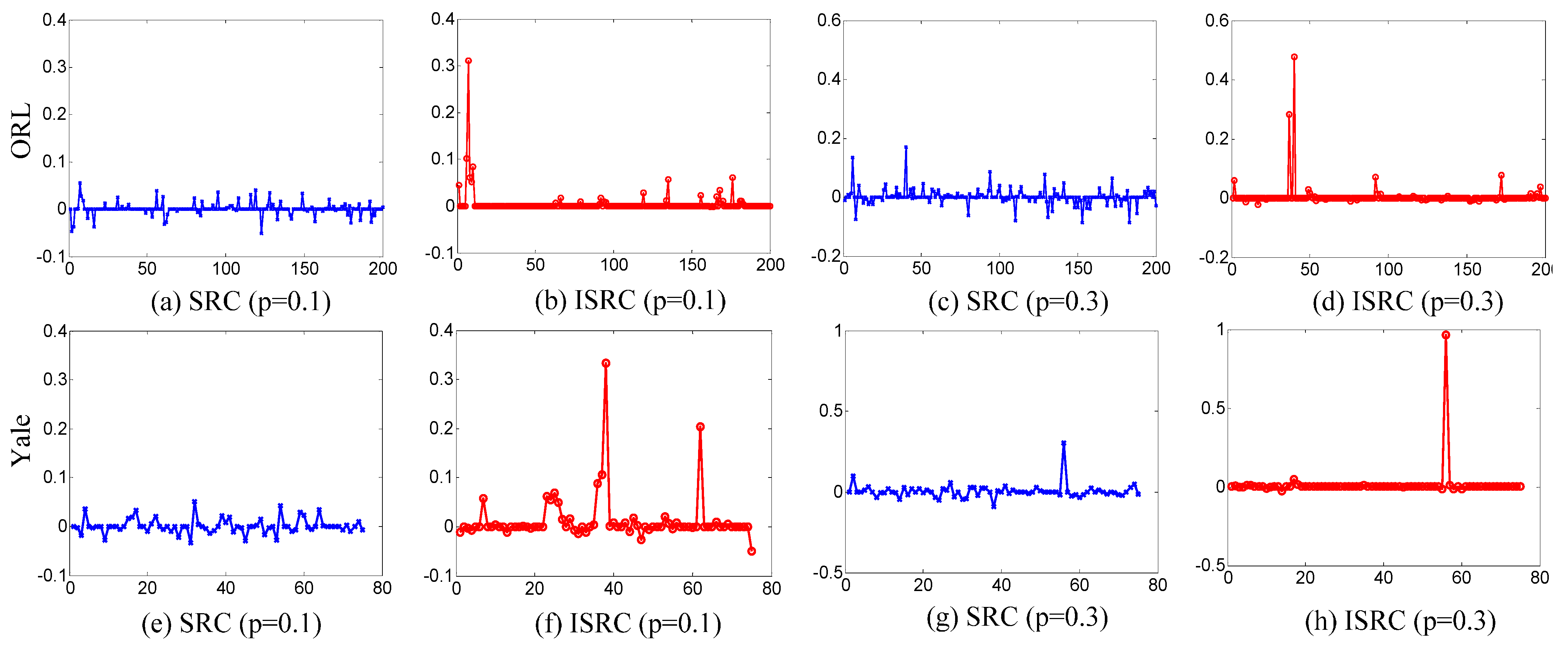
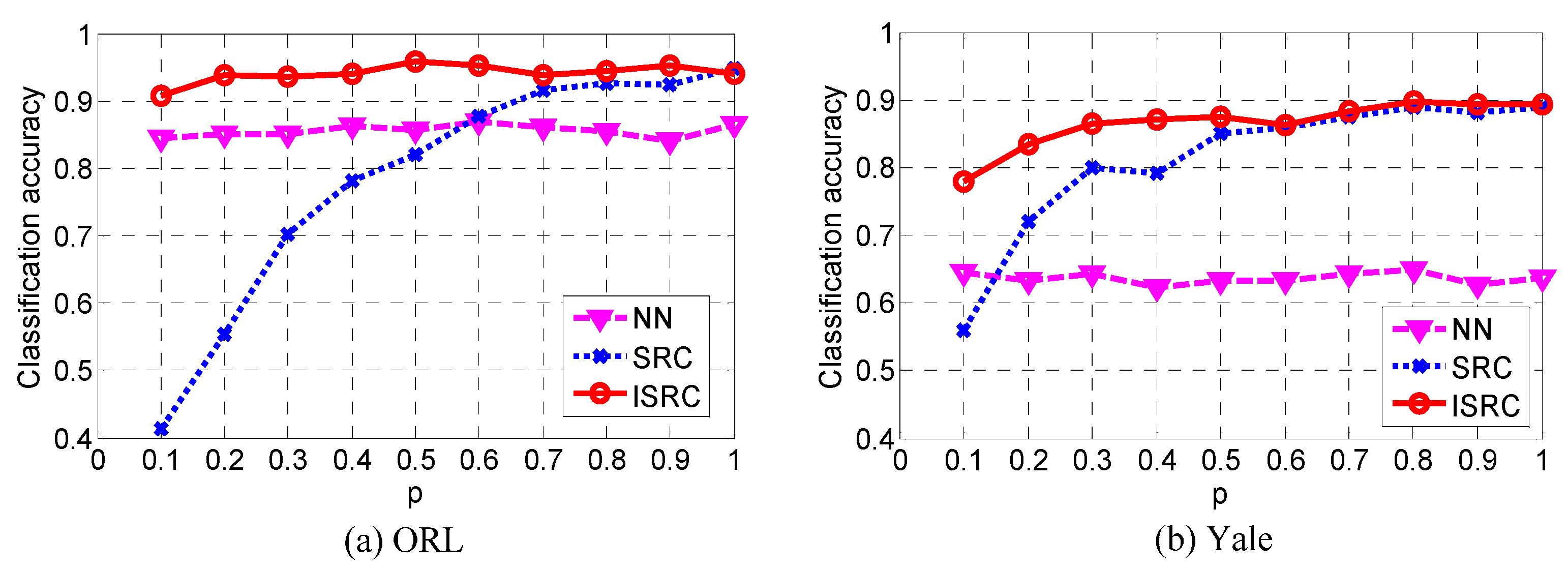
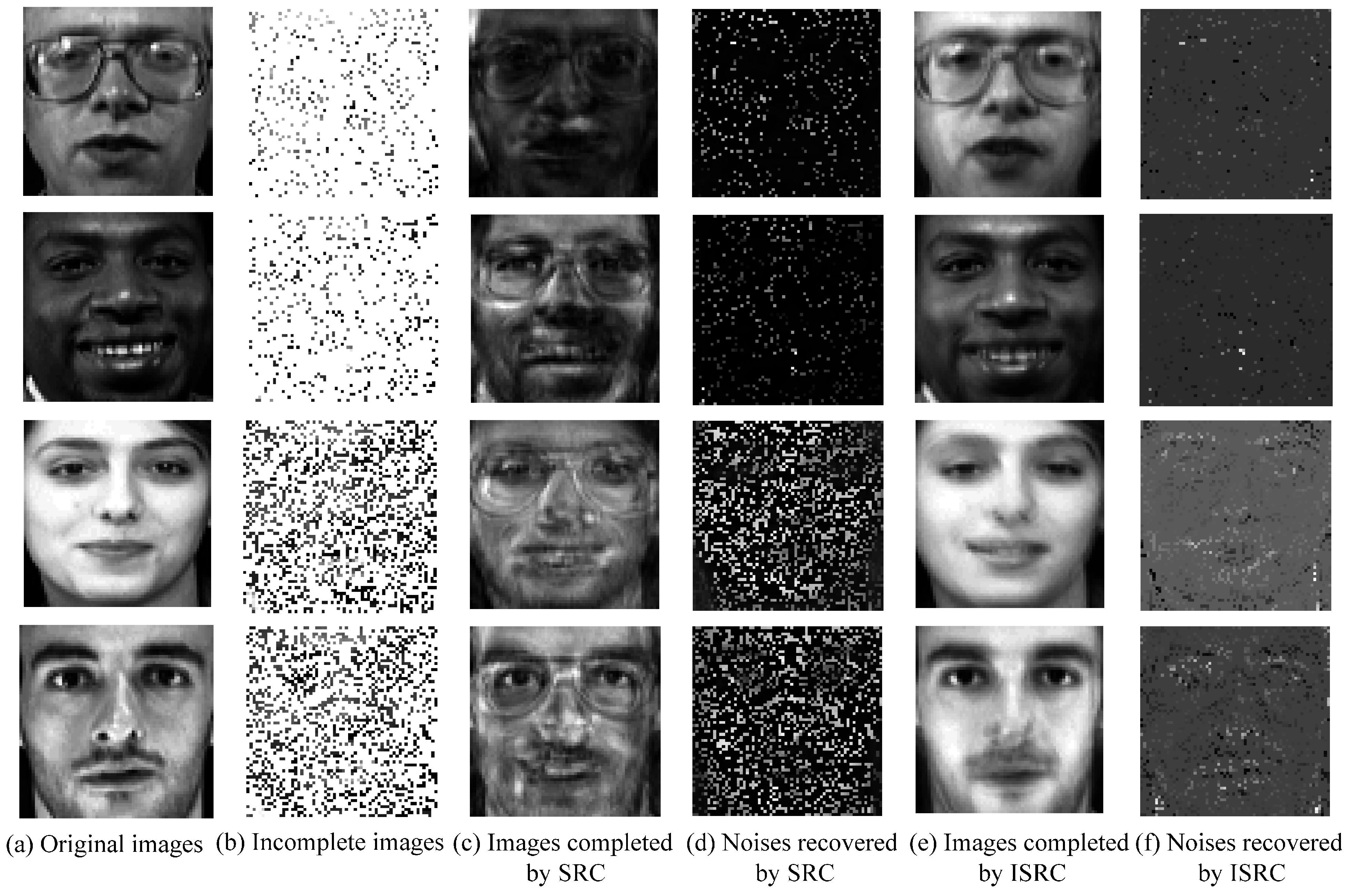
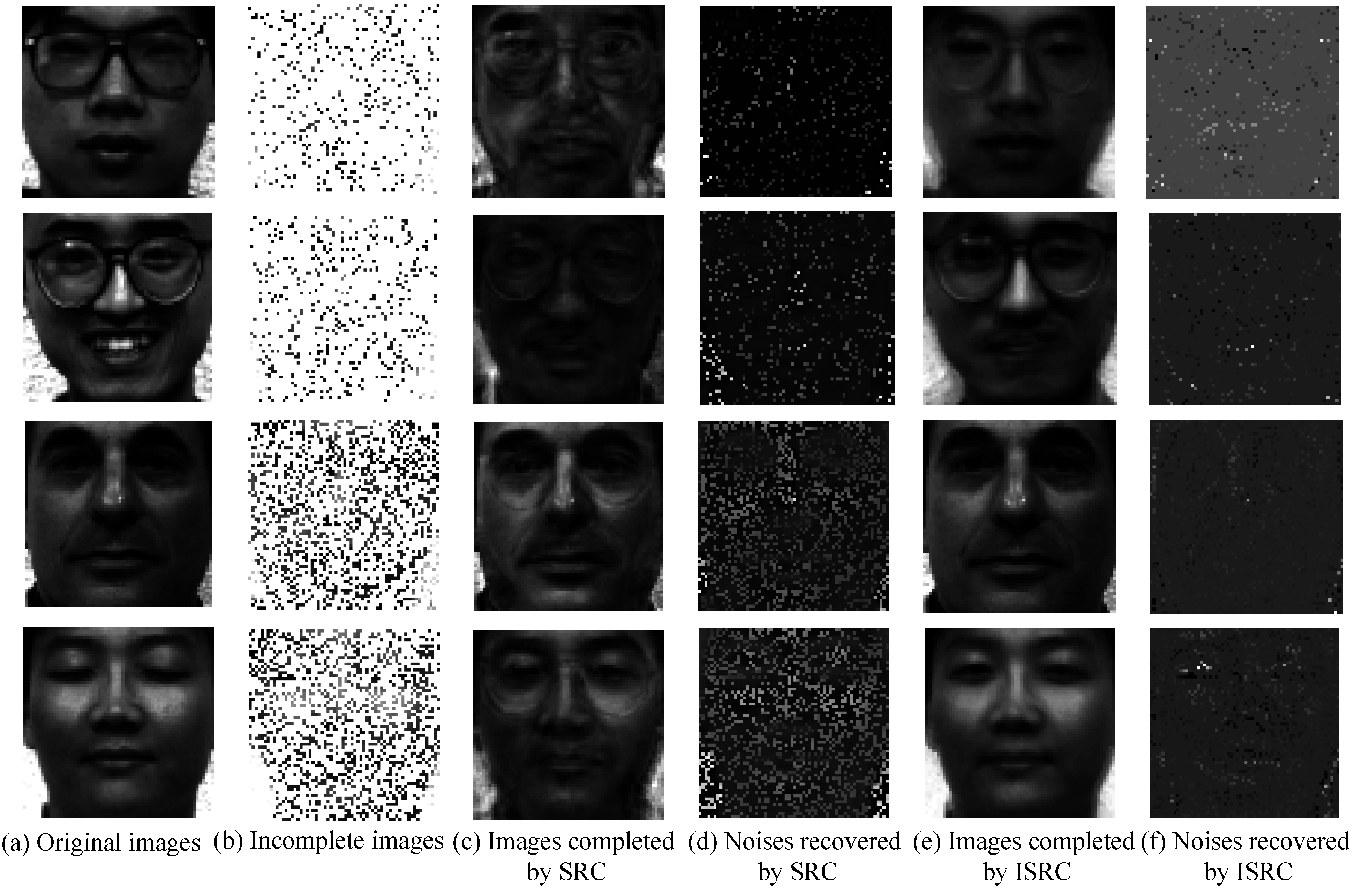
5.2. Experimental Analysis

We first compare the sparsity of the coefficient vectors obtained by SRC and ISRC respectively. Two different sampling probabilities are considered, that is, p = 0.1 and p = 0.3. The comparison results are partially shown in Figure 1. From this figure, we can see that each linear representation vector of ISRC has only a few relatively large components in the sense of absolute values and other values are close to zero. Compared with ISRC, SRC has worse sparsity performance due to the fact that its amplitude is relatively small. These observations show that ISRC has superiority over SRC in obtaining sparse representations.
Figure 1. Sparsity comparisons of the linear representations between SRC and ISRC.
Information 06 00287 g001
Then, we compare the classification performance of ISRC with that of SRC and NN on the two given datasets. To this end, we vary the values of p from 0.1 to 1 with an interval of 0.1. When p = 1, ISRC becomes SRC. Figure 2 shows the comparison results of classification accuracy, where (a) and (b) represent the results of ORL and Yale respectively. It can be seen from this figure that ISRC achieves the best classification accuracy compared with SRC and NN, and it is relatively stable for different values of p. SRC is very sensitive to the choice of p and its classification accuracy degenerates steeply with the decreasing of p. In addition, NN has lower classification accuracy although it is stable. To sum it up, ISRC is the most robust method and has the best classification performance.
Figure 2. Classification performance comparisons among NN, SRC and ISRC.
Information 06 00287 g002
For a test sample with missing values, both SRC and ISRC can recover all missing entries and noise to some extent. Finally, we compare their performance in completing missing entries and recovering the sparse noise. Here, we only consider two sampling probabilities, i.e., p = 0.1 and p = 0.3. For these two given probabilities, we compare the completed images and the recovered noise images obtained by SRC and ISRC respectively, as shown partially in Figure 3 and Figure 4.
Figure 3. Completion and recovery performance comparisons on ORL.
Information 06 00287 g003
Figure 4. Completion and recovery performance comparisons on Yale.
Information 06 00287 g004
In the above two figures, the sample probability is set to 0.1 in the first two lines of images and 0.3 in the latter two lines. For each figure, the first two columns of images display the original and the incomplete images respectively, where the positions with missing entries are shown in white. The third and the fifth columns of images give the completed images by SRC and ISRC respectively. The fourth and the last columns of images show the noise recovered by SRC and ISRC respectively. By comparing the completed images with the original images, we can see that ISRC not only has the better completion performance, but also automatically corrects the corruptions to a certain extent. Moreover, ISRC is more efficient in recovering noise than SRC. In summary, ISRC has better recovery performance than SRC.

6. Conclusions

This paper studies the problem of robust face classification with incomplete test samples. To address this problem, we propose a classification model based on incomplete sparse representation, which can be regarded as the generalization of sparse representation-based classification. Firstly, the incomplete sparse representation is described as an l1-minimization and the alternating direction method of multipliers is employed to solve this optimization problem. Then, we analyze the convergence of the proposed algorithm and extend the model to the case of a batch of test samples. Finally, the experimental results on two well-known face datasets demonstrate that the proposed classification method is very effective in improving classification performance and recovering the missing entries and noise. It still needs further research on the model and algorithm of incomplete sparse representation. In the future, we will consider the sparse representation-based classification problem that both training and testing samples have missing values.

Acknowledgments

This work is partially supported by the National Natural Science Foundation of China (No. 61403298, and No. 11401457), by the Natural Science Basic Research Plan in Shaanxi Province of China (No. 2014JQ8323), by the Shaanxi Provincial Education Department (No. 2013JK0587).

Author Contributions

Jiarong Shi constructed the model, developed the algorithm and wrote the manuscript. Xiuyun Zheng designed the experiments. Wei Yang implemented all experiments. All three authors were involved in organizing and refining the manuscript. All authors have read and approved the final manuscript.

Conflicts of Interest

The authors declare no conflict of interest.

References

  1. Donoho, D. Compressed sensing. IEEE Trans. Inf. Theory 2006, 52, 1289–1306. [Google Scholar] [CrossRef]
  2. Candès, E.J.; Michael, W. An introduction to compressive sampling. IEEE Signal Process. Mag. 2008, 25, 21–30. [Google Scholar] [CrossRef]
  3. Wright, J.; Yang, A.Y.; Ganesh, A.; Sastry, S.S.; Ma, Y. Robust face recognition via sparse representation. IEEE Trans. Pattern Anal. Mach. Intell. 2009, 31, 210–227. [Google Scholar] [CrossRef] [PubMed]
  4. Qiao, L.; Chen, S.; Tan, X. Sparsity preserving discriminant analysis for single training image face recognition. Pattern Recogn. Lett. 2010, 31, 422–429. [Google Scholar] [CrossRef]
  5. Zhang, S.; Zhao, X.; Lei, B. Robust facial expression recognition via compressive sensing. Sensors 2012, 12, 3747–3761. [Google Scholar] [CrossRef] [PubMed]
  6. Wright, J.; Ma, Y.; Mairal, J.; Sapiro, G.; Huang, T.; Yan, S. Sparse representation for computer vision and pattern recognition. Proc. IEEE 2010, 98, 1031–1044. [Google Scholar] [CrossRef]
  7. Cheng, B.; Yang, J.; Yan, S.; Fu, Y.; Huang, T. Learning with L1-graph for image analysis. IEEE Trans. Image Process. 2010, 19, 858–866. [Google Scholar] [CrossRef] [PubMed]
  8. Yin, J.; Liu, Z.; Jin, Z.; Yang, W. Kernel sparse representation based classification. Neurocomputing 2012, 77, 120–128. [Google Scholar] [CrossRef]
  9. Huang, K.; Aviyente, S. Sparse representation for signal classification. Neural Inf. Proc. Syst. 2006, 19, 609–616. [Google Scholar]
  10. Zhang, H.; Zha, Z.J.; Yang, Y.; Yan, S.; Chua, T.S. Robust (semi) nonnegative graph embedding. IEEE Trans. Image Process. 2014, 23, 2996–3012. [Google Scholar] [CrossRef] [PubMed]
  11. Chen, Y.; Zhang, S.; Zhao, X. Facial expression recognition via non-negative least-squares sparse coding. Information 2014, 5, 305–318. [Google Scholar] [CrossRef]
  12. Elhamifar, E.; Vidal, R. Sparse subspace clustering: Algorithm, theory, and applications. IEEE Trans. Pattern Anal. Mach. Intell. 2013, 35, 2765–2781. [Google Scholar] [CrossRef] [PubMed]
  13. Candès, E.J.; Recht, B. Exact matrix completion via convex optimization. Found. Comput. Math. 2009, 9, 717–772. [Google Scholar] [CrossRef]
  14. Shi, J.; Yang, W.; Yong, L.; Zheng, X. Low-rank representation for incomplete data. Math. Probl. Eng. 2014, 2014. [Google Scholar] [CrossRef]
  15. Boyd, S.; Parikh, N.; Chu, E.; Peleato, B.; Eckstein, J. Distributed optimization and statistical learning via the alternating direction method of multipliers. Found. Trends Mach. Learn. 2011, 3, 1–122. [Google Scholar] [CrossRef]
  16. Candès, E.J.; Li, X.; Ma, Y.; Wright, J. Robust principal component analysis? J. ACM 2011, 58. [Google Scholar] [CrossRef]
  17. ORL Database of Faces. Available online: http://www.cl.cam.ac.uk/research/dtg/attarchive/ facedatabase.html (accessed on 23 June 2015).
  18. Yale Face Database. Available online: http://vision.ucsd.edu/content/yale-face-database (accessed on 23 June 2015).

