Metric Learning with Dynamically Generated Pairwise Constraints for Ear Recognition
by
 , ,
, ,
Ibrahim Omara
1,2,* ,
,
Hongzhi Zhang
1,*,
Faqiang Wang
1,
Ahmed Hagag
3,
Xiaoming Li
1 and
Wangmeng Zuo
1 1
School of Computer Science and Technology, Harbin Institute of Technology, Harbin 150001, China
2
Department of Mathematics and computer Science, Faculty of Science, Menoufia University, Shebin El-kom 32511, Egypt
3
Faculty of Computers and Information, Banha University, Banha 13518, Egypt
*
Authors to whom correspondence should be addressed.
Information 2018, 9(9), 215; https://0-doi-org.brum.beds.ac.uk/10.3390/info9090215
Submission received: 8 August 2018
/
Revised: 23 August 2018
/
Accepted: 23 August 2018
/
Published: 27 August 2018
Abstract
:The ear recognition task is known as predicting whether two ear images belong to the same person or not. More recently, most ear recognition methods have started based on deep learning features that can achieve a good accuracy, but it requires more resources in the training phase and suffer from time-consuming computational complexity. On the other hand, descriptor features and metric learning play a vital role and also provide excellent performance in many computer vision applications, such as face recognition and image classification. Therefore, in this paper, we adopt the descriptor features and present a novel metric learning method that is efficient in matching real-time for ear recognition system. This method is formulated as a pairwise constrained optimization problem. In each training cycle, this method selects the nearest similar and dissimilar neighbors of each sample to construct the pairwise constraints and then solves the optimization problem by the iterated Bregman projections. Experiments are conducted on Annotated Web Ears (AWE) database, West Pommeranian University of Technology (WPUT), the University of Science and Technology Beijing II (USTB II), and Mathematical Analysis of Images (AMI) databases.. The results show that the proposed approach can achieve promising recognition rates in ear recognition, and its training process is much more efficient than the other competing metric learning methods.
1. Introduction
As an important person authentication technique, biometric recognition has been widely applied in surveillance applications, forensics, and criminal investigations. Since the biometric traits are unique, universal, and permanent, biometric recognition is more secure and reliable than traditional person authentication approaches.
Among the existing biometric recognition methods, there have been many kinds of biometric traits, e.g., face, fingerprint, palm-print, iris, signature, voice, key-stroke, and gait. Compared with the other traits, the human ear has a stable structure at different ages [1]. Additionally, the ear is insensitive to variations, such as make-up, glasses, and facial expression [2]. The ear image is also easy to acquire with little person awareness and user cooperation [3]. Furthermore, it has been proven that the left and right ears of the same person have some similarities but are not strictly symmetric [4]. Therefore, ear recognition has received increasing research interest.
Recently, for the ear recognition task, deep features [5,6,7] and learning methods have exploited and achieved better recognition rates than traditional handcrafted approaches. One of the most common methods is the metric learning method, which aims to learn the distance between two instances, where the distances between similar instances are shorter than those between dissimilar instances. Metric learning plays a crucial role in machine learning and has been successfully applied into many biometric recognition tasks, such as face recognition. Most of the existing metric learning methods learn the distance metric from the pairwise or triplet constraints [8]. The pairwise constraints make the distances of similar pairs shorter than a given threshold, while the distances of dissimilar pairs longer than this threshold. On the other hand, the triplet constraints make the distance of similar samples shorter than that of dissimilar samples. As the quantity of pairwise constraints is very large, pairs can be constructed from samples, the existing metric learning methods usually select part of the pairwise constraints for training. Davis et al. [9] proposed to select the pairwise constraints randomly. Wang et al. [10] proposed a strategy to construct the pairs from the training samples. For each training sample, its nearest similar and dissimilar samples are used to construct the similar and dissimilar pairs.
The previous metric learning methods construct the pairwise constraints as a preprocessing step and use the fixed pairwise constraints in training. This strategy, however, suffers from evident drawbacks. As the number of training pairs is fixed, and some pairs are never used in training, the trained models will under-fit the non-used training pairs. To address the aforementioned limitation, we propose a novel method to learn the distance metric from online generated pairwise constraints for an ear recognition system. First, it extracts the local phase quantization (LPQ), histogram of oriented gradient (HOG), and Gabor features of ear images. Then it uses the discriminant correlation analysis (DCA) method to fuse different features and reduce the feature dimension. Finally, it learns the distance metric based on the extracted feature. In this method, we learn the distance metric for several cycles. In each cycle, we construct the pairwise constraints by the trained distance in the last cycle and learn the distance metric based on these pairwise constraints. As the pairwise constraints are updated in each cycle, there are larger amount of training pairs utilized in our proposed method than the previous metric learning methods. We conduct the experiments on several ear image datasets, i.e., AWE, AMI, WPUT, and USTB databases, to evaluate our proposed method. The results show that our proposed method outperforms the state-of-the-art ear recognition approaches and most of the other competing metric learning methods in recognition accuracy and training time.
The rest of this paper is organized as follows: Section 2 introduces the related work about the commonly used ear recognition methods and metric learning algorithms. Section 3 demonstrates the proposed approach based on metric learning. Section 4 presents the experimental results, comparison on accuracy and training time, and offers a discussion of the results. Finally, Section 5 draws the conclusion of this paper.
2. Related Works
In this section, we give a brief review on the related works from two aspects, i.e., 2D ear recognition methods and metric learning algorithms.
2.1. 2D Ear Recognition
The existing works on 2D ear recognition system mainly focus on two aspects, i.e., feature extraction and classification. Three kinds of features, i.e., geometric, appearance-based, and deep neural network features, are mainly used in the ear recognition methods. The geometric features include maximum ear height line (EHL) [11,12], inner and outer helixes [11], tragus [13], etc. Lakshmanan [14] has presented a geometric approach based only the middle portion of the ear that adopted the reference line, normal lines, and angles. Some methods use the combination of these features [15,16] which can facilitate the discriminability of the geometric features. For the appearance-based features, it mainly includes intensity, directional and spatial-temporal information. Many of works have holistically presented features such as Eigen-ear and Eigen-face [2], independent component analysis (ICA) [17], and active shape model (ASM) to detect the outer ear contour [18], 1D and 2D Gabor filters [19,20], and locale features, such as local binary pattern (LBP) [21], HOG [22], scale invariant feature transform (SIFT) [23], and speeded up robust features (SURF) [24]. Recently, Nanni and Lumini [25] adopted the sequential forward floating selection (SFFS) to select the best features from sub-windows in an ear image. Yuan and Mu [26] presented a brief review of ear recognition and proposed a fusion method for ear recognition based on local features information. More recently, deep learning and convolutional neural networks (CNNs) have received more attention and achieved better performance for ear recognition problem; Pedro et al. [27] presented a personal neural network for ear recognition and explained a brief review for deep learning ear recognition. On the other hand, Omara et al. [5,28] exploited the pre-trained VGG-M model for extracting ear features, then fusion CNN features, and proposed a pairwise SVM classifier for ear classification. Emersic et al. [6] provided various CNN ear recognition models with limited training data based on the augmentation process of the training images to overcome the limited amount of labeled training data, and Dodge et al. [7] illustrated various deep CNNs as feature extractors and also adopted a shallow classifier for ear recognition. However, it is known that the deep learning methods have high feature dimensions and need more training computational complexity. Compared to deep features, local descriptors features need low computational complexity in both feature extraction and training because they have low feature dimensions.
For ear classification, we can notice that famous and typical ear recognition methods for 2D ear images focus on the feature extraction process and adopt a simple nearest neighbor, or typical SVM methods for ear recognition problems. Different distances are mainly adopted as the matching criterion, such as the Euclidean distance [15,29], Hamming distance [12,13,30], radial basis function (RBF) [17], back propagation (BP) network [11], and neural networks [31] and, recently, discriminative classifiers, such as approximate nearest neighbor (ANN) [32], support vector machine (SVM) [33,34], and pairwise SVM, have drawn much attention [5]. However, due to the lack of training images of ears and the multiple class properties of ear databases, typical matching processes may not lead to the desired performance whereas the Mahalanobis matrix takes the correlation of various features as the elements of the off-diagonal, and it is scale invariant. Therefore, an appropriate similarity distance metric should be considered in our proposed method. Called a Mahalanobis distance metric, it is learning over prior information to measure the similarity or dissimilarity between different instances. Therefore, we investigate an alternative method for ear recognition problem; metric learning extends the similarity measurement to take the advantage of prior information as a label over standard similarity measures. Metric learning has been proposed to learn Mahalanobis distance metrics for k-nearest neighbor classification and has better interclass generalization performance, which can be applied to handle the multiple classes of ear image databases better.
2.2. Metric Learning
Metric learning plays a crucial role for various applications in computer vision and machine learning applications, such as signature verification [35], data classification [36], and person re-identification [37]. The existing metric learning can be divided into two categories, i.e., pairwise constrained metric learning and triplet constrained metric learning. The pairwise constrained metric learning methods include information-theoretic metric learning (ITML) [9], logistic discriminant metric learning (LDML) [38], distance metric learning with eigenvalue (DML-eig) [39], and sparse metric learning (SML) [40], etc. The ITML method formulates the problem as minimizing the LogDet divergence instance between the learned distance metric and prior distance metric subject to the pairwise constraints [9]. It can be solved by the iterated Bregman projection algorithm. Guilllaumin et al. [38] proposed the LDML method. It defines the probabilities of each sample pair to be similar and dissimilar, respectively, and formulates the problem as maximizing the log-likelihood of all training pairs. Ying et al. proposes the DML-eig method formulated their metric learning as an eigenvalue optimization problem with pairwise constraints [39]. Kostinger et al. [41] proposes the KISSME method to learn the distance metric from the equivalence constraints. Its training is a one-pass process and doesn’t need any iteration.
In addition to the pairwise constrained metric learning methods, some other methods learn the metric based on the triplet constraint. This causes each sample to be close to its similar sample and far from its dissimilar sample. Large margin nearest neighbor (LMNN) learns the distance metric by a convex problem with triplet constraints [42]. It separates the similar and dissimilar neighbors of each sample by a large margin. Shen et al. propose the BoostMetric [43], MetricBoost [44], and FrobMetric [45] methods. They parameterize the distance metric as the linear combination of rank-one matrices and learn the combination parameters based on triplet constraints. The construction of pairwise or triplet constraints is crucial to the performance of metric learning methods. Among the existing metric learning methods, many methods construct the constraints by randomly selecting the pairs or triplets. Wang et al. [10] propose a nearest neighbor strategy to construct the pairs and triplets and proved that this strategy can lead to higher recognition accuracy than the random selection strategy. However, the pairs and triplets are fixed in their training process. In our work, we train the model for many cycles , and we dynamically update the pairwise constraints by the nearest neighbor strategy in each cycle as shown in Figure 1, where is the distance threshold. Thus, our proposed method can incorporate more pairwise constraints in training for learning the distance function.
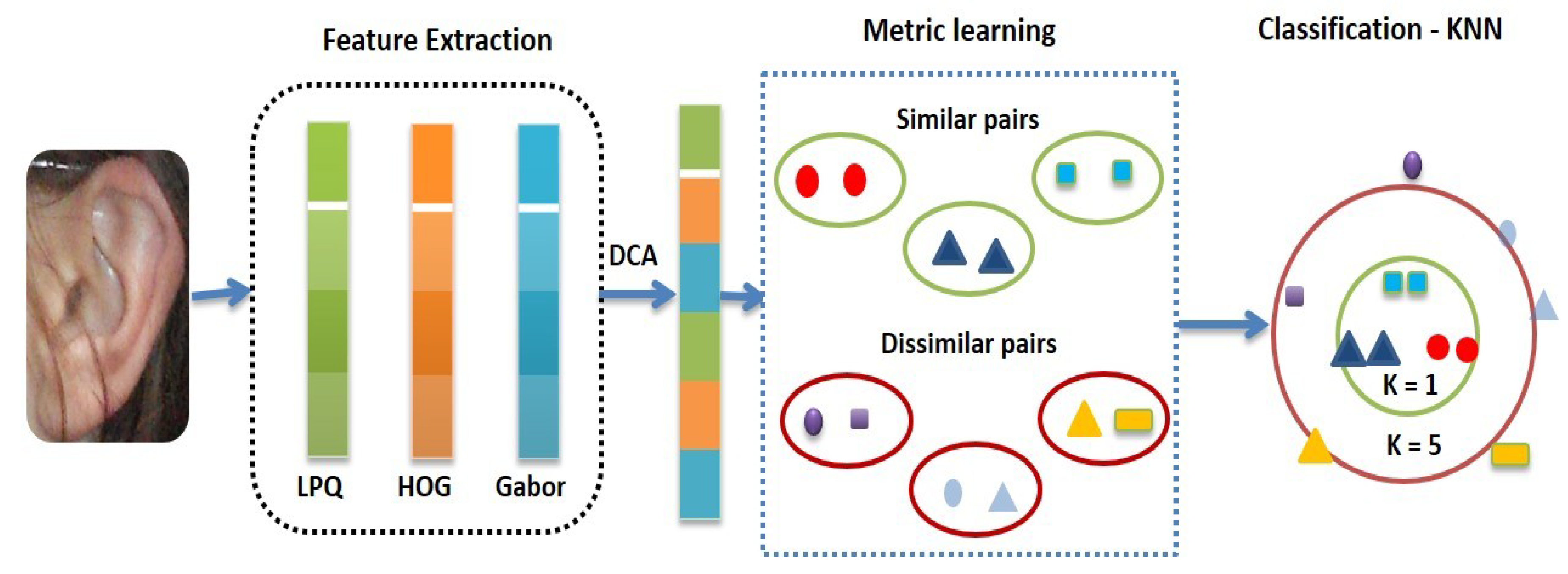
3. Proposed Method
In this section, we illustrate the proposed method, ear recognition based on the LogDet divergence (ERLD) method, for an ear recognition system. Following a similar preprocessing phase for all approaches, where the geometrical properties of the ears are mostly flat, the proposed method first resizes all images to a fixed size of 100 × 100 pixels and applies histogram equalization to the resized image, since various ear databases such as the AWE database have different ear image sizes and the local descriptors require aligning images before the feature extraction phase. Then, for feature extractions, it uses the local phase quantization (LPQ), histogram of oriented gradient (HOG), and Gabor feature techniques as used in [46] to represent the ear images. Afterward, it adopts a discriminant correlation analysis (DCA) algorithm [47] to fuse and reduce the feature dimension. Finally, it learns a Mahalanobis distance metric by using the proposed dynamically pairwise constraints based on the extracted feature and applies KNN for ear matching and classification. The sketch of the proposed method is illustrated in Figure 2. In details for description LPQ, HOG, and Gabor features are as follows: In the LPQ descriptor, the proposed approach uses a window size of 5 × 5, and the block size is 18 × 18 pixels without block overlap. In the HOG descriptor, the proposed approach adopts a cell of 8 × 8 pixels, and the block size is 16 × 16 pixels with an overlap of eight pixels. Finally, for Gabor features, the number of orientations is fixed to eight with five scales and 40 filters and a down-sampling value of 64. In addition, discriminant correlation analysis (DCA) is a feature-level fusion algorithm and it considers the class structure in feature fusion. It also includes the class associations in the correlation analysis of the feature sets and performs an effective feature fusion based on maximizing the pair-wise correlations across the two feature vectors. DCA also reduces the between-class correlations and restricting the correlations to be within classes (for more details of DCA, see [47]). Therefore, our approach exploits the advantages of the DCA algorithm for the feature fusion and limitation dimension problem.
3.1. Problem Formulation
Given n training samples where , is the feature of the training sample, the squared Mahalanobis distance between is defined as Equation (1):
where is the distance metric which is a positive semi-definite matrix.
Denote by are from the same person} the set of similar pairs and are from different people} the set of dissimilar pairs. We hope the pairs satisfy the following constraints shown in Equation (2):
where U and L are the upper and lower thresholds.
Similar with ITML [9], we formulate the objective function as that of minimizing the LogDet divergence function to make the learned distance metric to be close to the given prior distance metric . Thus, the problem is formulated as Equation (3):
where is the LogDet divergence function between two matrices and [9,48]. is the trace of the matrix, and is the dimension of training samples. Both the proposed method and ITML [9] are fast and scalable because they do not require any eigenvalue computations or semi-definite programming. However, the constraints of the ITML model are fixed and strict, which may require more iteration to achieve convergence. Therefore, the ITML method suffers from suboptimal performance since it may not learn the most appropriate from the fixed pairwise constraints which are used to improve the accuracy of a k-nearest neighbor classifier. On the other hand, the proposed method tries to solve the previous issues by using cycles to select the most appropriate constraints for learning the distance faster without requiring more learning iterations. In other words, the proposed method can achieve better performance and improve the accuracy of the KNN classifier, and is faster than the ITML method based on updating the pairwise constraints through several cycles to learn the distance metric, as shown in Figure 1.
3.2. Training Algorithm
3.2.1. Construction of the Pairwise Constraints
For constructing the pairwise constraints, most of previous metric learning methods construct the pairwise constraints as a preprocessing step and use the fixed pairwise constraints in training, such as ITML [9]. To address the previous issues, the proposed metric learning algorithm adopts dynamically generated pairwise constraints based on a cyclic projection method to seek an optimized kernel matrix under linear inequality constraints. In detail, suppose that there are training samples , where . The proposed method initializes the similar and dissimilar pair sets in the first cycle, and then updates the pair sets in each of the rest cycles. Denoted by and the sets of similar and dissimilar pairs and the learned distance metric in the cycle, respectively. In the first cycle, we initialize as the identity matrix, compute the Euclidean distance of every two training samples, and then find the nearest similar and dissimilar neighbors of each sample to initialize , respectively. In the cycle, we use as the prior distance metric to compute the Mahalanobis distances of every two training samples. Based on the distances, we find the nearest similar and dissimilar neighbors of each sample to sets , respectively.
3.2.2. Optimization of the Distance Metric
In each training cycle, we set the prior distance metric as , and solve Equation (3) with the training pairs . Following [9], we initialize as , and learn the distance metric by repeatedly compute the Bregman projections as follows:
where is a training pair in , and is the Lagrange multiplier corresponding to pair .
3.2.3. The proposed metric learning algorithm
As described in Section 3.2.1 and Section 3.2.2, we can summarize the algorithm of the proposed method as Algorithm 1. Since and refer to the distance matrix, the similar and dissimilar pairs, respectively. For training the proposed model, the model trains for many cycles , and we dynamically update the pairwise constraints by the nearest neighbor strategy in each cycle to incorporate more pairwise constraints in training for learning the distance function and to ensure the Mahalanobis distance is optimized. This means, in each cycle, the proposed metric learning algorithm generates a new pairwise constraint to optimize the Mahalanobis metric distance step by step from to , and is the iterative Mahalanobis metric at cycle . Therefore, the proposed algorithm computes the convergence factor between the prediction and target (desired Mahalanobis) metrics, i.e., , where is a threshold. If the convergence factor achieves the required threshold, the proposed algorithm then adopts the present Mahalanobis distance as a target metric for training the model. On other hand, if the convergence factor does not achieve the required threshold, then the proposed algorithm updates the pairwise constraints and Mahalanobis metric as shown in Figure 1 and Algorithm 1 until it achieves the convergence factor. Where is the Lagrange multiplier corresponding to pair is a regularization parameter that balances the regularization function and , and are the initial and desired distances, respectively, that are used to classify the instances as similar and dissimilar.
| Algorithm 1. The training algorithm of the proposed method. |
| Input: Training set , cycle number Output: Learned distance metric . Step 1. Initialize the prior distance metric as the identity matrix. Step 2. For 2.1. 2.2. Compute the distances of every two training samples with the distance metric . Step 3. For each training sample : 3.1. Find the nearest similar and dissimilar neighbors of as and . 3.2. 3.3. End for (Step 3) Step 4. 4.1. Repeat 4.2. Pick a pair in 4.3. . 4.4. . 4.5. 4.6. 4.7. 4.8. 4.9. Until convergence Step 5. 5.1. End for Step 6. Return |
4. Datasets and Experimental Results
To evaluate our proposed method, the experiments are conducted on four public and complicated ear databases, i.e., Annotated Web Ears (AWE) database [46], West Pommeranian University of Technology (WPUT) [49], the University of Science and Technology Beijing II (USTB II) [11] and Mathematical Analysis of Images (AMI) [50] databases.
4.1. Datasets
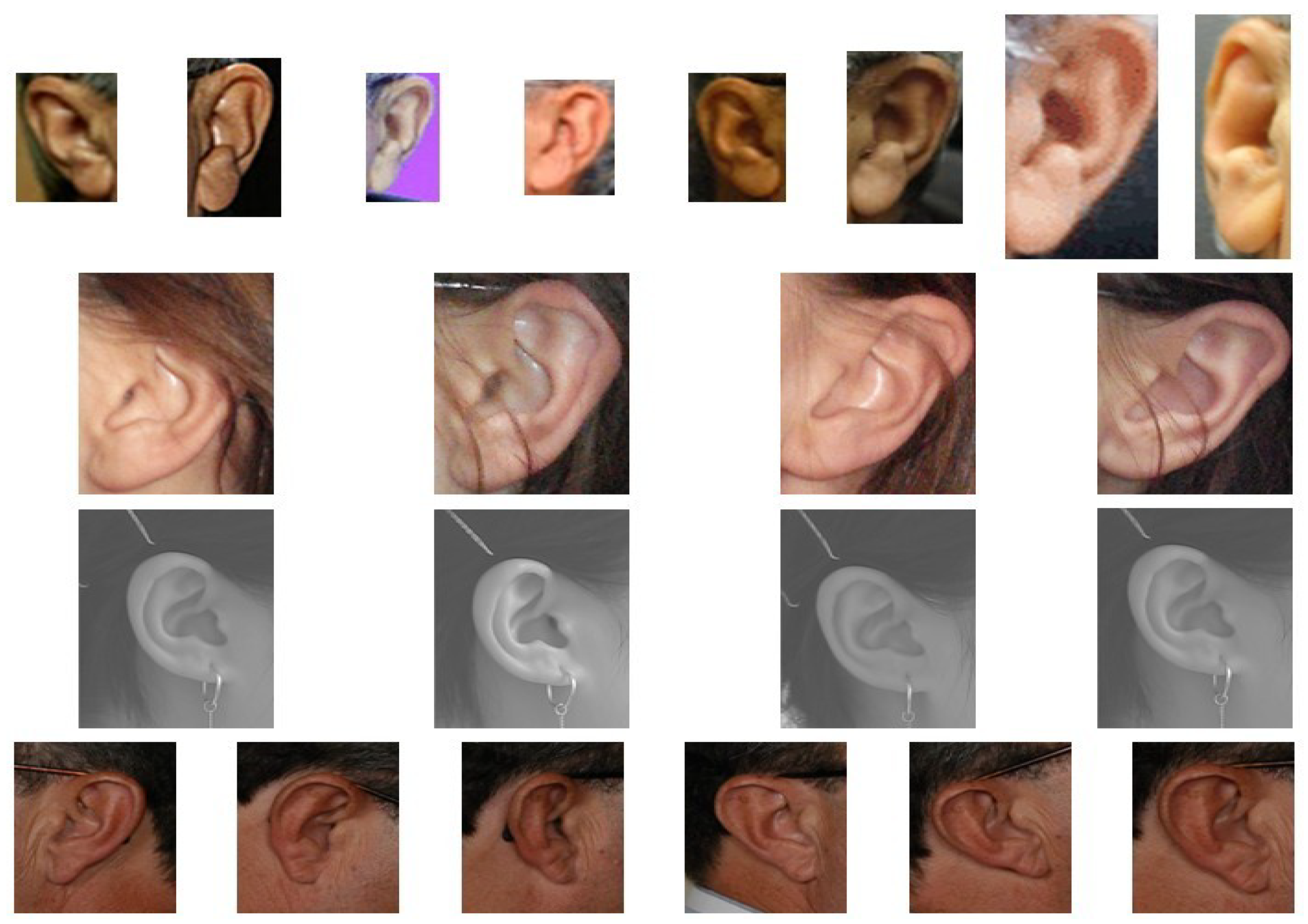
First, the AWE database [46] includes 100 subjects and it is collected from the internet with high degree of variability and various illuminations, and with different scales and rotations. All AWE images were manually inspected, and each person has 10 images that were selected for inclusion in the dataset. Second, the WPUT database [49] was introduced in 2010 and consists of 3345 images of 475 persons with 1388 duplicates, among which each person has 4–10 images; we are used only four images for each subject. The WPUT images are taken from men and women, and under different indoor lightning conditions and head rotation angles ranging from approximately 90° for profile to 75°, and occlusions include earrings, hats, tattoos, etc., for more difficulty. Third, the USTB II database [11] contains 308 images of 77 persons, which are taken under different illumination and camera views. Each person has four images. The first image is the frontal ear image under standard illumination, the second and the third images are taken with +30 and −30 rotations respectively, and the fourth image is taken under weak illumination. Finally, the AMI database [50] has 700 images from 100 persons, all of subjects in the age range of 19–65 years. AMI ear images were collected from students, teachers, and staff at Universidad de Las Palmas de Gran Canaria (ULPGC), Las Palmas, Spain, and taken in an indoor environment. Each person has seven images; five of them were right side profile (right ear) and the sixth image of right profile was taken but with a different camera, and the last image was taken from a left side profile (left ear). Figure 3 shows the original ear images for one subject from each database.
4.2. Experiment Settings
The experiments are conducted on four complicated public ear databases, AWE, WPUT, USTB2, and AMI databases. For comprising and evaluating the proposed metric learning method with state-of-the-art ear recognition methods and metric learning algorithms, we partition each of the AWE, USTB2, AMI, and WPUT databases into two sets, one for training and the other for testing. The training dataset randomly contains 60% of the ear images from each database and the remainder, i.e., 40%, from each database for testing. We also use ten pairs in each cycle, which the number of cycles is 10 for the learning distance function of the proposed method. All experiments are performed with MATLAB R2016a software and on a computer with 3.4 GHz Intel Xeon E3-1230 CPU V2 and 32 GB for RAM.
4.3. Comparison of Accuracy with Existing Ear Recognition Systems
In this subsection, we compare the proposed method with the state-of-the-art ear recognition methods, the Euclidean distance, and the traditional Mahalanobis distance with the inverse covariance matrix as the distance metric on the recognition accuracy, as shown in Table 1. For our experiments, all experiments are performed 10 times for illustrating the robustness and efficiency of the proposed method and the results illustrate the mean and standard deviation of the system performance for each database. Table 1 shows the comparable results of our proposed methods to existing ear recognition systems from the literature. The results show the superior of our proposed method than other methods by large margin, due to this large margin on the results of the proposed method that is based on learning a Mahalanobis distance for ear recognition system, we firstly evaluate the ear recognition system based on different metric learning state-of-the-art methods as will illustrate in the following subsection.
4.4. Comparison of Metric Learning Methods on Accuracy and Training Time
To illustrate our proposed method’s ability to learn a distance function, we compare it to some existing metric learning methods in the literature. To the best of our knowledge, we firstly exploit metric learning methods to evaluate the accuracy on the ear recognition system; different databases with the same setting and protocol are used in this evaluation. Moreover, we compare the proposed metric learning method with the state-of-the-art metric learning methods, i.e., ITML [9], LMNN [42], LDML [38], and LDMLT [53] on recognition rate and training time as shown in Table 2, Table 3, Table 4 and Table 5 for the AWE, USTB2, WPUT, and AMI databases, respectively. We follow the same previous protocol and repeat our experiments 10 times and report the mean recognition accuracy and standard deviation by using the K-nearest neighbor (K-NN) classifier with K = 1, 2, …5. It may be observed that our proposed method can achieve better performances than the other competing methods in the WPUT and USTB II databases in Table 3 and Table 4, even if the WPUT and USTB II databases are small-scale, meaning that the metric learning methods based on triplet constraints cannot achieve good performance with a small ear training dataset. Moreover, the training results time on four databases show the superior of the proposed method. On the other hand, when the ear training dataset increased, such as in the AWE and AMI databases, the recognition rates of our proposed method are slightly lower than those of LMNN and LDML. That is because LDMLT and LMNN are based on triplet constraints which provide more information of the data, but it requires higher computational complexity. While our proposed method, which is based on dynamically pairwise constraints, can provide good information and can apply to real-time application as shown on the training time in Table 2, Table 3, Table 4 and Table 5 for the AWE, USTB2, WPUT, and AMI databases, respectively.
4.5. Discussion
The metric learning methods in the literature include two types of constraints, pairwise and triplet constraints. For pairwise constraints, the metric learning methods learn the distance metric by selecting a random part of the pairwise constraints while the quantity of all constraints is very large: pair for samples or instances. In this regard, ITML [9] and LDML [38] methods randomly select the pairwise constraints for each iteration. Then, it uses the fixed constraints to update the metric learning matrix, while this fixed constraint may not be provided a critical metric learning matrix for solving the problem, and not achieve the desired convergence that leads to training more iterations for adopting a good result. On other hand, the metric learning methods make each instance to be close to its similar instance and far from dissimilar instance for building triplet constraints . These methods, such as LMNN [42] and LDMLT [53], use a number of cycles to update the triplet constraints every cycle, and to achieve the critical learning matrix that is play a vital role in classification problem. However, the metric learning methods LMNN and LDMLT have complicated triplet constraints and need more computational complexity for training. Therefore, the proposed metric learning method exploits the advantages of pairwise constraints besides updating it by the nearest neighbor strategy through several cycles to achieve a critical metric learning matrix and obtain promising results with a short time as shown in previous subsections. Moreover, we can notice that the training time of our proposed method is much shorter than the other metric learning methods. We analyzed the computational complexity of our proposed method in training. From Equation (3), the computational complexity of each iteration is . However, as there are m cycles and pairs in each cycle, the computational complexity of our proposed method is .
5. Conclusions
Recently, most researchers have gained more attention working on unconstrained ear recognition, which is a very challenging problem. Most previous ear recognition methods are based on the feature extraction phase and used traditional classifiers for ear matching. More recently, metric learning methods have achieved a promising performance on various applications, such as face recognition, signature verification, data classification, and person re-identification. Therefore, in this paper, we firstly propose a novel pairwise constrained metric learning method for unconstrained ear recognition. In this method, we update the pairwise constraint using the nearest neighbor strategy in each training cycle and learn the distance metric via minimizing the LogDet divergence of the learned metric and prior metric. This method can incorporate more pairwise constraints to learn the distance metric, which can improve the recognition performance with efficient training time. The experiments are conducted on challenging and complicated ear databases, such as AWE, AMI, WPUT, and USTB II databases. The results show that our proposed method can achieve favorable recognition accuracy compared with the state-of-the-art ear recognition methods, and its training time is much faster than the other competing metric learning methods. In the future, we will investigate applying this strategy to dynamically build the triplet constraint and propose more metric learning methods for ear recognition system. In addition, we will try to propose other methods for identical twins based on the fusion of handcrafted and deep features by using ear images. Moreover, we will investigate a simple convolutional neural network for ear recognition with more occlusion.
Author Contributions
I.O. provided all the results together with proofs, and figures. H.Z. and F.W. extended the analysis and simplified some formulation. The first two authors wrote Section 4. I.O. and F.W. proposed the metric learning algorithm, contributed to model formalization, checked the proofs, and wrote Section 1 and Section 2. A.H., X.L. and W.Z. improved writing Section 1 and Section 2. In addition, W.Z. is a project administration.
Funding
This work was supported by the National Natural Science Foundation of China under grant Nos. 61271093 and 61471146.
Acknowledgments
This work is a part by the co-operation between Higher Education Commission of Egypt and Chinese Government.
Conflicts of Interest
The authors declare no conflict of interest.
References
- Ibrahim, M.I.; Nixon, M.S.; Mahmoodi, S. The effect of time on ear biometrics. In Proceedings of the International Joint Conference on Biometrics (IJCB), Washington, DC, USA, 11–13 October 2011; pp. 1–6. [Google Scholar] [CrossRef]
- Chang, K.; Bowyer, K.W.; Sarkar, S.; Victor, B. Comparison and combination of ear and face images in appearance-based biometrics. IEEE Trans. Pattern Anal. Mach. Intell. 2003, 25, 1160–1165. [Google Scholar] [CrossRef] [Green Version]
- Burge, M.; Burger, W. Using ear biometrics for passive identification. In Proceedings of the IFIP TC11 14th International Conference on Information Security, Vienna, Austria, Budapest, Hungary, 31 August–2 September 1998; pp. 139–148. [Google Scholar]
- Abaza, A.; Ross, A. Towards understanding the symmetry of human ears: A biometric perspective. In Proceedings of the 2010 Fourth IEEE International Conference on Biometrics: Theory, Applications and Systems (BTAS), Washington, DC, USA, 27–29 September 2010; pp. 1–7. [Google Scholar]
- Omara, I.; Wu, X.; Zhang, H.; Du, Y.; Zuo, W. Learning pairwise SVM on hierarchical deep features for ear recognition. IET Biom. 2018. [Google Scholar] [CrossRef]
- Emeršič, Ž.; Štepec, D.; Štruc, V.; Peer, P. Training convolutional neural networks with limited training data for ear recognition in the wild. arXiv, 2017; arXiv:1711.09952. [Google Scholar]
- Dodge, S.; Mounsef, J.; Karam, L. Unconstrained ear recognition using deep neural networks. IET Biom. 2018, 7, 207–214. [Google Scholar] [CrossRef]
- Bellet, A.; Habrard, A.; Sebban, M. A survey on metric learning for feature vectors and structured data. ArXiv, 2013; arXiv:1306.6709. [Google Scholar]
- Davis, J.V.; Kulis, B.; Jain, P.; Sra, S.; Dhillon, I.S. Information-theoretic metric learning. In Proceedings of the 24th international conference on Machine learning, Corvallis, OR, USA, 20–24 June 2007; pp. 209–216. [Google Scholar]
- Wang, F.; Zuo, W.; Zhang, L.; Meng, D.; Zhang, D. A kernel classification framework for metric learning. IEEE Trans. Neural Netw. Learn. Syst. 2015, 26, 1950–1962. [Google Scholar] [CrossRef] [PubMed]
- Mu, Z.; Yuan, L.; Xu, Z.; Xi, D.; Qi, S. Shape and structural feature based ear recognition. In Advances in Biometric Person Authentication; Springer: Berlin/Heidelberg, Germany, 2004; pp. 663–670. [Google Scholar]
- Shailaja, D.; Gupta, P. A simple geometric approach for ear recognition. In Proceedings of the Information Technology, International Conference on (2006), Bhubaneswar, India, 18–27 December 2006; pp. 164–167. [Google Scholar]
- Annapurani, K.; Sadiq, M.A.K.; Malathy, C. Fusion of shape of the ear and tragus—A unique feature extraction method for ear authentication system. Expert Syst. Appl. 2015, 42, 649–656. [Google Scholar] [CrossRef]
- Lakshmanan, L. Efficient person authentication based on multi-level fusion of ear scores. IET Biom. 2013, 2, 97–106. [Google Scholar] [CrossRef]
- Omara, I.; Li, F.; Zhang, H.; Zuo, W. A novel geometric feature extraction method for ear recognition. Expert Syst. Appl. 2016, 65, 127–135. [Google Scholar] [CrossRef]
- Rahman, M.; Sadi, M.S.; Islam, M.R. Human ear recognition using geometric features. In Proceedings of the 2013 International Conference on Electrical Information and Communication Technology (EICT 2013), KUET, Khulna, Bangladesh, 19–21 December 2013; pp. 1–4. [Google Scholar]
- Zhang, H.J.; Mu, Z.C.; Qu, W.; Liu, L.M.; Zhang, C.Y. A novel approach for ear recognition based on ICA and RBF network. In Proceedings of the 2005 International Conference on Machine Learning and Cybernetics, Guangzhou, China, 18–21 August 2005; pp. 4511–4515. [Google Scholar]
- Yuan, L.; Mu, Z.C. Ear recognition based on 2D images. In Proceedings of the 2007 First IEEE International Conference on Biometrics: Theory, Applications and Systems, Crystal City, Virginia, 27–29 September 2007; pp. 1–5. [Google Scholar]
- Nanni, L.; Lumini, A. Fusion of color spaces for ear authentication. Pattern Recogn. 2009, 42, 1906–1913. [Google Scholar] [CrossRef]
- Kumar, A.; Wu, C. Automated human identification using ear imaging. Pattern Recogn. 2012, 45, 956–968. [Google Scholar] [CrossRef]
- Boodoo-Jahangeer, N.B.; Baichoo, S. LBP-based ear recognition. In Proceedings of the 2007 First IEEE International Conference on Biometrics: Theory, Applications and Systems, Crystal City, Virginia, 27–29 September 2007; pp. 1–4. [Google Scholar]
- Damer, N.; Führer, B. Ear recognition using multi-scale histogram of oriented gradients. In Proceedings of the Intelligent Information Hiding and Multimedia Signal Processing (IIH-MSP), Piraeus-Athens, Greece, 18–20 July 2012; pp. 21–24. [Google Scholar]
- Zhou, J.; Cadavid, S.; Abdel-Mottaleb, M. Exploiting color sift features for 2d ear recognition. In Proceedings of the 2011 18th IEEE International Conference on Image Processing, Brussels, Belgium, 11–14 September 2011; pp. 553–556. [Google Scholar]
- Prakash, S.; Gupta, P. An efficient ear recognition technique invariant to illumination and pose. Telecommun. Syst. 2013, 52, 1435–1448. [Google Scholar] [CrossRef]
- Nanni, L.; Lumini, A. A multi-matcher for ear authentication. Pattern Recogn. Lett. 2007, 28, 2219–2226. [Google Scholar] [CrossRef]
- Yuan, L.; chun Mu, Z. Ear recognition based on local information fusion. Pattern Recogn. Lett. 2012, 33, 182–190. [Google Scholar] [CrossRef]
- Galdámez, P.L.; Raveane, W.; Arrieta, A.G. A brief review of the ear recognition process using deep neural networks. J. Appl. Log. 2016, 24, 62–70. [Google Scholar] [CrossRef]
- Omara, I.; Wu, X.; Zhang, H.; Du, Y.; Zuo, W. Learning pairwise SVM on deep features for ear recognition. In Proceedings of the 16th IEEE/ACIS International Conference on Computer and Information Science, Wuhan, China, 24–26 May 2017; pp. 341–346. [Google Scholar]
- Ghoualmi, L.; Draa, A.; Chikhi, S. An ear biometric system based on artificial bees and the scale invariant feature transform. Expert Syst. Appl. 2016, 57, 49–61. [Google Scholar] [CrossRef]
- Chan, T.S.; Kumar, A. Reliable ear identification using 2-D quadrature filters. Pattern Recogn. Lett. 2012, 33, 1870–1881. [Google Scholar] [CrossRef]
- Sanchez, D.; Melin, P. Optimization of modular granular neural networks using hierarchical genetic algorithms for human recognition using the ear biometric measure. Eng. Appl. Artif. Intell. 2014, 27, 41–56. [Google Scholar] [CrossRef]
- Omara, I.; Emam, M.; Hammad, M.; Zuo, W. Ear verification based on a novel local feature extraction. In Proceedings of the 2017 International Conference on Biometrics Engineering and Application, Hong Kong, China, 21–23 April 2017; pp. 28–32. [Google Scholar]
- Yaqubi, M.; Faez, K.; Motamed, S. Ear recognition using features inspired by visual cortex and support vector machine technique. In Proceedings of the International Conference on Computer and Communication Engineering, Kuala Lumpur, Malaysia, 13–15 May 2008; pp. 533–537. [Google Scholar]
- Benzaoui, A.; Hadid, A.; Boukrouche, A. Ear biometric recognition using local texture descriptors. J. Electron. Imaging 2014, 23, 053008. [Google Scholar] [CrossRef]
- Soleimani, A.; Araabi, B.N.; Fouladi, K. Deep multitask metric learning for offline signature verification. Pattern Recogn. Lett. 2016, 80, 84–90. [Google Scholar] [CrossRef]
- Xiang, S.; Nie, F.; Zhang, C. Learning a Mahalanobis distance metric for data clustering and classification. Pattern Recogn. 2008, 41, 3600–3612. [Google Scholar] [CrossRef]
- Liong, V.E.; Lu, J.; Ge, Y. Regularized local metric learning for person re-identification. Pattern Recogn. Lett. 2015, 68, 288–296. [Google Scholar] [CrossRef]
- Guillaumin, M.; Verbeek, J.; Schmid, C. Is that you? Metric learning approaches for face identification. In Proceedings of the 2009 IEEE 12th International Conference on Computer Vision (ICCV), Kyoto, Japan, 24 September–4 October 2009; pp. 498–505. [Google Scholar]
- Ying, Y.; Li, P. Distance metric learning with eigenvalue optimization. J. Mach. Learn. Res. 2012, 13, 1–26. [Google Scholar]
- Ying, Y.; Huang, K.; Campbell, C. Sparse metric learning via smooth optimization. In Proceedings of the Advances in Neural Information Processing Systems, Vancouver, BC., Canada, 7–10 December 2009; pp. 2214–2222. [Google Scholar]
- Koestinger, M.; Hirzer, M.; Wohlhart, P.; Roth, P.M.; Bischof, H. Large scale metric learning from equivalence constraints. In Proceedings of the 25th IEEE Conference on Computer Vision and Pattern Recognition, Providence, Rhode Island, 16–21 June 2012; pp. 2288–2295. [Google Scholar]
- Weinberger, K.Q.; Saul, L.K. Distance metric learning for large margin nearest neighbor classification. J. Mach. Learn. Res. 2009, 10, 207–244. [Google Scholar]
- Shen, C.; Kim, J.; Wang, L.; Hengel, A. Positive semidefinite metric learning with boosting. In Proceedings of the Advances in Neural Information Processing Systems, Vancouver, BC, Canada, 7–10 December 2009; pp. 1651–1659. [Google Scholar]
- Shen, C.; Kim, J.; Wang, L.; Hengel, A.V.D. Positive semidefinite metric learning using boosting-like algorithms. J. Mach. Learn. Res. 2012, 13, 1007–1036. [Google Scholar]
- Shen, C.; Kim, J.; Wang, L. A scalable dual approach to semidefinite metric learning. In Proceedings of the 2011 IEEE Conference on Computer Vision and Pattern Recognition (CVPR), Colorado Springs, CO, USA, 20–25 June 2011; pp. 2601–2608. [Google Scholar]
- Emeršic, Ž.; Štruc, V.; Peer, P. Ear recognition: More than a survey. Neurocomputing 2017, 255, 26–39. [Google Scholar] [CrossRef] [Green Version]
- Haghighat, M.; Abdel-Mottaleb, M.; Alhalabi, W. Discriminant correlation analysis: Real-time feature level fusion for multimodal biometric recognition. IEEE Trans. Inf. Forensics Secur. 2016, 11, 1984–1996. [Google Scholar] [CrossRef]
- Kulis, B.; Sustik, M.A.; Dhillon, I.S. Low-rank kernel learning with Bregman matrix divergences. J. Mach. Learn. Res. 2009, 10, 341–376. [Google Scholar]
- Frejlichowski, D.; Tyszkiewicz, N. The west pomeranian university of technology ear database–a tool for testing biometric algorithms. Image Anal. Recogn. 2010, 227–234. [Google Scholar]
- Gonzalez, E.; Alvarez, L.; Mazorra, L. Mathematical Analysis of Images (AMI) Ear Database. Available online: http://www.ctim.es/research_works/ami_ear_database/ (accessed on 10 August 2017).
- Raghavendra, R.; Raja, K.B.; Busch, C. Ear recognition after ear lobe surgery: A preliminary study. In Proceedings of the IEEE International Conference on Identity, Security and Behavior Analysis, Sendai, Japan, 29 February–2 March 2016; pp. 1–6. [Google Scholar]
- Hansley, E.E.; Segundo, M.P.; Sarkar, S. Employing fusion of learned and handcrafted features for unconstrained ear recognition. IET Biom. 2018, 7, 215–223. [Google Scholar] [CrossRef] [Green Version]
- Mei, J.; Liu, M.; Karimi, H.R.; Gao, H. Logdet divergence based metric learning using triplet labels. In Proceedings of the 30th International Conference on International Conference on Machine Learning, Atlanta, GA, USA, 16–21 June 2013. [Google Scholar]
Figure 1.
Diagram of the dynamic pairwise constraints. It shows the convergence of similar pairs (squares) and divergence of dissimilar pairs (circles) by updating pairwise constraints.
Figure 1.
Diagram of the dynamic pairwise constraints. It shows the convergence of similar pairs (squares) and divergence of dissimilar pairs (circles) by updating pairwise constraints.

Figure 2.
The sketch of the proposed ear recognition method.

Figure 3.
Original ear images for one subject from AWE (first row), WPUT (second row), USTB II (third row), and AMI (fourth row).
Figure 3.
Original ear images for one subject from AWE (first row), WPUT (second row), USTB II (third row), and AMI (fourth row).


Table 1.
Comparison on recognition rate (%) for the AWE, USTB2, AMI, and WPUT databases.
| Methods | AWE | USTB2 | AMI | WPUT | |
|---|---|---|---|---|---|
| Emersic et al. [46] | 49.6 ± 6.80 | 90.9 ± 6.50 | -- | -- | |
| Raghavendra et al. [51] | -- | -- | 86.36 | -- | |
| Benzaoui et al. [34] | -- | 90.9 ± 6.50 | 47.72 | -- | |
| Earnest et al. [52] | 90.60 | -- | -- | EER = 9.40 | |
| Samuel et al. [7] | 85.00 | -- | -- | -- | |
| Ours | Mahalanobis distance | 72.22 ± 1.93 | 91.71 ± 5.11 | 95.50 ± 1.19 | 57.00 ± 1.83 |
| Metric learning | 98.13 ± 0.72 | 95.85 ± 3.90 | 96.65 ± 1.36 | 93.42 ± 2.06 | |
Table 2.
The average of recognition rate (%) and training time for different metric learning methods in the AWE database.
Table 2.
The average of recognition rate (%) and training time for different metric learning methods in the AWE database.
| Methods | Time | K = 1 | K = 2 | K = 3 | K = 4 | K = 5 |
|---|---|---|---|---|---|---|
| ITML [9] | 59.68 s | 83.38 ± 5.62 | 72.23 ± 7.22 | 70.68 ± 8.35 | 69.70 ± 7.96 | 69.5 ± 8.25 |
| LMNN [42] | 148.75 s | 99.25 ± 0.72 | 99.25 ± 0.72 | 99.23 ± 0.82 | 99.23 ± 0.83 | 98.88 ± 1.11 |
| LDML [38] | 18.29 s | 99.10 ± 0.01 | 99.10 ± 0.01 | 99.10 ± 0.01 | 99.05 ± 0.01 | 99.10 ± 0.01 |
| LDMLT [53] | 9.68 s | 98.95 ± 0.86 | 98.95 ± 86 | 99.18 ± 0.8 | 99.35 ± 0.86 | 99.35 ± 0.85 |
| Ours | 2.13 s | 98.13 ± 0.72 | 98.13 ± 0.72 | 98.70 ± 0.39 | 98.75 ± 0.50 | 98.80 ± 0.61 |
Table 3.
The average of recognition rate (%) and training time for different metric learning methods in the USTB2 database.
Table 3.
The average of recognition rate (%) and training time for different metric learning methods in the USTB2 database.
| Methods | Time | K = 1 | K = 2 | K = 3 | K = 4 | K = 5 |
|---|---|---|---|---|---|---|
| ITML [9] | 17.67 s | 93.33 ± 4.51 | 80.33 ± 3.65 | 75.37 ± 3.97 | 73.17 ± 4.28 | 69,51 ± 4.97 |
| LMNN [42] | 19.70 s | 94.07 ± 3.72 | 94.07 ± 3.72 | 78.78 ± 3.22 | 78.78 ± 3.22 | 57.32 ± 8.78 |
| LDML [38] | 13.25 s | 93.09 ± 3.59 | 93.09 ± 3.59 | 92.44 ± 3.49 | 91.87 ± 3.68 | 91.71 ± 3.73 |
| LDMLT [53] | 15.64 s | 94.96 ± 2.7 | 94.96 ± 2.7 | 94.88 ± 2.66 | 94.88 ± 2.66 | 94.63 ± 3.05 |
| Ours | 11.77 s | 95.85 ± 3.90 | 95.85 ± 3.90 | 95.77 ± 3.82 | 95.37 ± 4.08 | 95.37 ± 4.35 |
Table 4.
The average of recognition rate (%) and training time for different metric learning methods in the WPUT database.
Table 4.
The average of recognition rate (%) and training time for different metric learning methods in the WPUT database.
| Methods | Time | K = 1 | K = 2 | K = 3 | K = 4 | K = 5 |
|---|---|---|---|---|---|---|
| ITML [9] | 140.12 s | 91.80 ± 2.20 | 91.80 ± 2.20 | 91.95 ± 2.21 | 91.85 ± 2.16 | 91.72 ± 2.12 |
| LMNN [42] | 3346.9 s | 93.75 ± 1.96 | 93.75 ± 1.96 | 88.64 ± 2.15 | 88.64 ± 2.15 | 78.32 ± 3.19 |
| LDML [38] | 95.29 s | 93.07 ± 0.02 | 93.07 ± 0.02 | 88.16 ± 0.02 | 83.89 ± 0.03 | 79.91 ± 0.05 |
| LDMLT [53] | 173.36 s | 92.45 ± 2.17 | 92.45 ± 2.17 | 92.37 ± 2.18 | 92.2 ± 2.15 | 91.92 ± 2.14 |
| Ours | 12.15 s | 93.42 ± 2.06 | 93.42 ± 2.07 | 93.30 ± 2.04 | 92.88 ± 2.03 | 92.36 ± 2.19 |
Table 5.
The average of recognition rate (%) and training time for different metric learning methods in the AMI database.
Table 5.
The average of recognition rate (%) and training time for different metric learning methods in the AMI database.
| Methods | Time | K = 1 | K = 2 | K = 3 | K = 4 | K = 5 |
|---|---|---|---|---|---|---|
| ITML [9] | 54.91 s | 97.64 ± 0.66 | 96.29 ± 1.31 | 95.89 ± 1.69 | 96.04 ± 1.72 | 96.19 ± 1.76 |
| LMNN [42] | 58.15 s | 99.12 ± 1.03 | 99.12 ± 1.03 | 98.07 ± 1.47 | 98.07 ± 1.47 | 95.21 ± 2.22 |
| LDML [38] | 5.43 s | 98.79 ± 1.09 | 98.79 ± 1.09 | 98.32 ± 1.17 | 97.86 ± 1.31 | 97.32 ± 1.75 |
| LDMLT [53] | 1.21 s | 98.04 ± 1.61 | 98.04 ± 1.61 | 98.32 ± 1.21 | 98.32 ± 1.14 | 98.39 ± 1.07 |
| Ours | 0.74 s | 96.96 ± 1.36 | 96.96 ± 1.36 | 97.12 ± 1.43 | 97.61 ± 1.53 | 97.76 ± 1.38 |
© 2018 by the authors. Licensee MDPI, Basel, Switzerland. This article is an open access article distributed under the terms and conditions of the Creative Commons Attribution (CC BY) license (http://creativecommons.org/licenses/by/4.0/).
Share and Cite
MDPI and ACS Style
Omara, I.; Zhang, H.; Wang, F.; Hagag, A.; Li, X.; Zuo, W. Metric Learning with Dynamically Generated Pairwise Constraints for Ear Recognition. Information 2018, 9, 215. https://0-doi-org.brum.beds.ac.uk/10.3390/info9090215
AMA Style
Omara I, Zhang H, Wang F, Hagag A, Li X, Zuo W. Metric Learning with Dynamically Generated Pairwise Constraints for Ear Recognition. Information. 2018; 9(9):215. https://0-doi-org.brum.beds.ac.uk/10.3390/info9090215
Chicago/Turabian StyleOmara, Ibrahim, Hongzhi Zhang, Faqiang Wang, Ahmed Hagag, Xiaoming Li, and Wangmeng Zuo. 2018. "Metric Learning with Dynamically Generated Pairwise Constraints for Ear Recognition" Information 9, no. 9: 215. https://0-doi-org.brum.beds.ac.uk/10.3390/info9090215
Note that from the first issue of 2016, this journal uses article numbers instead of page numbers. See further details here.