Imbalanced Learning Based on Data-Partition and SMOTE

School of Computer and Information Technology, Xinyang Normal University, Xinyang 464000, China
*
Author to whom correspondence should be addressed.
Information 2018, 9(9), 238; https://0-doi-org.brum.beds.ac.uk/10.3390/info9090238
Submission received: 5 August 2018
/
Revised: 13 September 2018
/
Accepted: 17 September 2018
/
Published: 19 September 2018
(This article belongs to the Section Artificial Intelligence)
Abstract
:Classification of data with imbalanced class distribution has encountered a significant drawback by most conventional classification learning methods which assume a relatively balanced class distribution. This paper proposes a novel classification method based on data-partition and SMOTE for imbalanced learning. The proposed method differs from conventional ones in both the learning and prediction stages. For the learning stage, the proposed method uses the following three steps to learn a class-imbalance oriented model: (1) partitioning the majority class into several clusters using data partition methods such as K-Means, (2) constructing a novel training set using SMOTE on each data set obtained by merging each cluster with the minority class, and (3) learning a classification model on each training set using convention classification learning methods including decision tree, SVM and neural network. Therefore, a classifier repository consisting of several classification models is constructed. With respect to the prediction stage, for a given example to be classified, the proposed method uses the partition model constructed in the learning stage to select a model from the classifier repository to predict the example. Comprehensive experiments on KEEL data sets show that the proposed method outperforms some other existing methods on evaluation measures of recall, g-mean, f-measure and AUC.
1. Introduction
Class-imbalanced problems is an important research field in machine learning and pattern recognition [1], and, for two-class problems, the imbalanced data is characterized as the size of one class (minority class or positive class) is much smaller than that of the contrary one (majority class or negative class) [2]. In many practical applications, correctly classifying the minority class examples is often of greater importance than correctly classifying the contrary ones. For example, in fraud detection, only few cases are the fraud cases and how to correctly identify the fraud cases is very meaningful [3]. Although classification methods, such as k-nearest neighbor (KNN), decision tree, support vector machine (SVM) and back-propagation neural network, have been widely used in many real-world applications to guild decision-making, classifying imbalanced data still challenges these conventional classification models. The reasons include (1) when facing the imbalanced circumstance, standard approaches often provide a good coverage of the majority class examples, distorting the minority class examples [4], (2) the learning process guided by measures such as global accuracy leads to an overlooking to the minority class examples [5], (3) minority class examples may be misclassified into noise and vice versa, since both of them are the rare class in the data space [6] and (4) minority class examples may overlap with other classes, which causes minority class examples often being misclassified into the majority class [7].
Many approaches have been proposed to handle the class-imbalanced problems. These approaches can be mainly categorized into two levels: data level approaches and algorithm level approaches. Approaches at data level try to rebalance the data distribution by sampling the data space such that the conventional learning methods can capture the characteristics of the minority class [8,9,10,11,12,13,14,15,16,17]. Approaches at the algorithm level try to improve the generalization ability of existing algorithms on imbalanced data by adjusting the learning process of the algorithms. In this manner, these approaches require clear comprehension of the algorithm itself and its application domains, knowing why the algorithm performs poorly when the data distribution is imbalanced. Existing methods at this level include enhancing the discriminatory ability of classifiers using kernel transformation [18] and converting the learning objective to functions which punish errors on the minority class more severely [19].
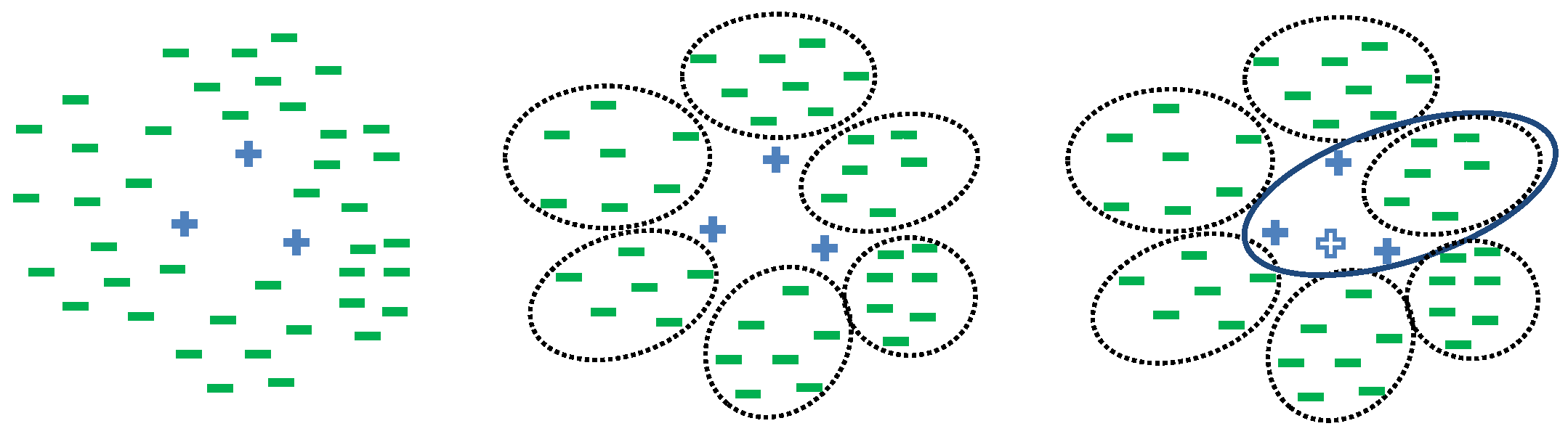
This paper proposes a novel classification method based on data-partition and an oversampling technique, namely SMOTE [10], for imbalanced learning. In the learning stage, the proposed method firstly pre-processes the training set using partition methods and SMOTE: using partition methods such as K-Means [20] to partition the majority class into several clusters, and create a new training set using SMOTE to oversample each data set obtained by merging the minority class with each cluster. Then, the proposed method learns a classification model on each novel training set, and therefore a repository of classification models is constructed. In the prediction stage, the method uses a partition model obtained in the learning stage to distribute an unlabeled example into a cluster, and the corresponding classification model is selected. The idea of partitioning the majority set is inspired by the intuition that the new training set obtained through operations of partition, merging and over-sampling is more balanced and separable. For example, the model (such as SVM) learned on the data set shown in the left sub-figure of Figure 1 intuitively tends to predict the positive class samples to be negative ones. After partitioning the negative class set to several clusters, the model learned from the novel data set obtained by merging the positive class and each cluster (the example set in solid ellipse of the right sub-figure of Figure 1) is more prone to correctly classifying the three positive class examples, as the novel data set is separable. The right sub-figure of Figure 1 also shows that the new training set obtained after the over-sampling operation (the hollow cross represents an example generated by SMOTE) can further improve the performance of conventional methods on imbalanced data. Therefore, the main contributions of this work are as follows:
- proposing a data-partition based method to enhance separability between majority class and minority class, and thus improving the performance of conventional methods on class-imbalance data;
- combining an oversampling technique, namely SMOTE, with a data-partition method through oversampling the partitioned data to obtain a more balanced one, and thus further enhancing the performance of traditional methods on imbalanced problems;
- extensive experiments are conducted and the corresponding results show that the proposed method significantly outperforms the other state-of-the-art methods on measures of recall, g-mean, f-measure and AUC.
The rest of the paper is organized as follows. After presenting the related work in Section 2, Section 3 describes the proposed method for class-imbalanced problem, followed by the discussion of parameters learning in Section 4 and the experimental results in Section 5. Finally, Section 6 concludes the paper.
2. Related Work
2.1. Characteristics of Imbalanced Data
The imbalanced data set that exhibits an unequal distribution between its classes can be considered imbalanced (skewed). Theoretical and empirical results indicate that, besides the skewed data distribution, many factors influence the classifier performance on identifying the minority class examples [21]. These factors include imbalanced class distribution, small sample size, class overlapping and within-class subconcepts.
- Imbalanced Class Distribution: The imbalance degree of a data set is often denoted by the ratio of the size of the majority class to that of the minority class. The studies carried out by Weiss and Provostin [22] showed that the model constructed on a relatively balanced distribution usually obtains a better classification performance. However, it is difficult to explicitly state at what imbalance degree the class distribution would deteriorate the classification performance due to other factors including class overlapping and within-class subconcepts also affecting the performance.
- Small Sample Size: For a data with a given imbalance degree, the data size determines the performance of a classification model. If the data size is small, limited examples of the minority class can not cover the inherent regularities. The studies carried out by Japkowicz and Stephen [23] indicated that, providing a large enough data set, the imbalanced class distribution may not affect the classification performance. However, in practice, collecting sufficient data for class imbalanced data sets is challenging [24].
- Class Overlapping: Class overlapping is the major issue that causes the difficulty of separating the minority class from the majority class. Simple rules can be induced to distinguish class examples if there are highly discriminative patterns existing in the examples among different classes. However, if the examples belonging to different classes overlap, it is hard for discriminative models to be induced, and, in most cases, examples belonging to the minority class are incorrectly classified to the contrary cases.
- Within-Class Subconcepts: Within-class subconcepts mean that the examples of a class are collected from various subconcepts and the size of these subconcepts may be different. The existing of within-class concepts increases the learning concept complexity on the imbalanced data set [25].
2.2. Sampling Technique
The sampling technique including under-sampling, over-sampling and clustering-based sampling is one of the most popular methods to solve the problem existing in imbalanced data [26,27]. The approaches of the under-sampling technique aim to balance the data distribution by eliminating majority class examples. Random under-sampling, a commonly used sampling method, randomly discards majority class examples until a relatively balanced distribution is reached. The problem existing in random under-sampling is that useful examples may be eliminated leading to a worse classification performance [28]. To overcome this drawback, many methods have been proposed to retain useful information presented in the majority class. Examples include the condensed nearest neighbor (CNN) rule [29] and Tomek Links [30], where CNN tries to remove redundant examples of the majority class and Tomek Links is to discard borderline and noisy examples.
The approaches of the over-sampling technique is to rebalance the data distribution by creating a new minority class, and random over-sampling is one of the most widely used over-sampling methods. In random over-sampling, majority class examples are randomly duplicated such that the class distribution is more balanced. Though the over-sampling technique creates more balanced distribution, it suffers from the drawback of overfitting [28]. The synthetic minority over-sampling technique (SMOTE) [10] was proposed to overcome this drawback, which synthetically generates new minority class examples along the line between the two selected minority class samples. Borderline over-sampling [31] only oversamples the borderline minority class samples since the borderline region is more crucial for establishing the decision boundary. The majority weighted minority oversampling technique (MWMOTE) [14] identifies the hard-to-learn informative minority samples, assigns weights according to their distances from the nearest majority class samples, and generates synthetic samples from the weighted minority class samples. Some other over-sampling methods such as Borderline-SMOTE [32] and Safe-level-SMOTE [33] were also proposed to handle overfitting.
In recent years, many clustering-based sampling approaches have been proposed for handling class-imbalanced problem, such as Sobhani [12] dividing the majority class into several clusters and selecting at least one sample from each cluster to form a subset of the majority class with the size equal to the minority class. Yen [13] partitioned the whole training set into several clusters, and selected majority class samples from each cluster according to the ratio of the size of the majority class to that of the minority class, and combined the selected majority class samples with the minority class samples to obtain a new training set. Prachuabsupakij [34] proposed a method that partitions the training set into two clusters, uses over-sampling and under-sampling to resample each cluster, learns a random forest on each resampled cluster, and obtains the prediction on an example by combining the results from both clusters through a majority vote.
Our method differs from the above methods both in the learning and prediction stages: for the learning stage, our method first partitions the majority class into several clusters, and directly combines the minority class with each cluster as a new cluster, applies SMOTE to oversample each new cluster, and, based on each new cluster, a conventional classification model is learned. Therefore, a classifier lab with a size equal to partition number is constructed. For the prediction stage, the partition method learned in the learning stage is used to select the corresponding classification model for prediction and thus our method is a special single model instead of an ensemble one.
2.3. Clustering
The process of grouping a set of examples into classes of similar characteristic is called clustering. A cluster is a collection of examples within which the examples are similar to each other and are dissimilar to examples of other clusters [35]. Many clustering algorithms have been proposed, and partition based clustering and hierarchical clustering are commonly used methods.
Partition-based clustering constructs k partitions of the examples, where each partition represents a cluster. These clusters should fulfill the following requirements: (1) each cluster must contain at least one object, and (2) each example must belong to exactly one cluster. K-Means is widely used in many practical applications because of its simplicity and adaptability [36]. In the K-Means algorithm, a center is the average of all points in a partition. Other commonly used partition based clustering methods including ISODATA [37] and PAM [38].
Hierarchical clustering (HC) algorithms organize data into a hierarchical structure according to the proximity matrix [39]. HC could be mainly categorized into two groups: agglomerative methods and divisive methods. Agglomerative methods start with N clusters and each cluster is composed of only one example and then iteratively merges the two closest clusters until the pre-determined number of cluster is reached. Contrary to agglomerative methods, divisive methods start with the entire data set as one cluster and iteratively divides the most appropriate cluster, and repeats the dividing process until a pre-specified criterion is reached.
2.4. Evaluation Measures
Evaluation measures play a key role in both accessing the performance of the classification model and the guiding of its modeling process [25]. Traditional evaluation measures such as accuracy focus more on the majority class examples, ignoring the minority class examples that are relative to the user preference [28]. For example, in a problem where the minority class contains 1% of all the examples, a naive approach predicting all examples to be the majority class would achieve an accuracy of 99%. Though 99 percentage accuracy appears good on the whole data set, all of the minority class examples are misclassified.
Table 1 presents the confusion matrix of the prediction of a classifier on biclass problem. Based on Table 1, many measures including recall, precision, f-measure and g-mean have been designed for the class-imbalanced problem. Recall and precision are defined as:
F-measure is s a harmonic mean between recall and precision, when the relative importance between recall and precision is set to 1, f-measure becomes f1-measure, formally
Like f-measure, g-mean is another metric considering both minority class and majority class. Specifically, g-mean measures the balanced performance of a classifier using the geometric mean of the recall of minority class and that of majority class. Formally, g-mean is as follows:
In addition, AUC is a commonly used measure to evaluate model performance. According to [28], AUC can be estimated by
In this paper, we apply recall, g-mean, f-measure, AUC and precision as candidate measures to evaluate the generalization ability of the proposed method.
3. Imbalanced Learning Based on Data-Partition and SMOTE
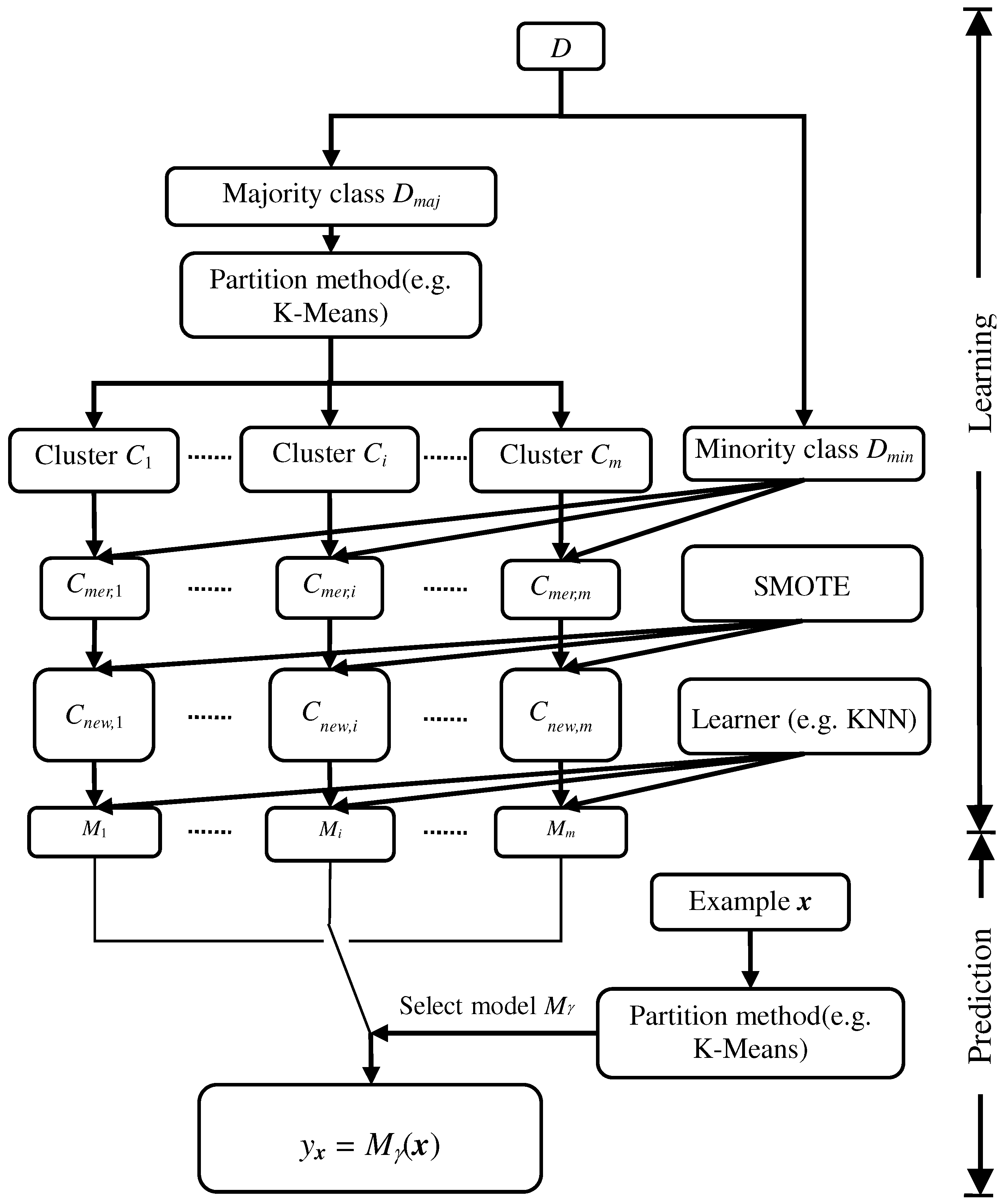
In this paper, a novel imbalanced learning method based on data-partition and SMOTE is proposed, which is a method of data level approaches for class-imbalanced problems. Figure 2 illustrates the learning and prediction stages of the proposed method. Different from other existing methods, in the learning stage, the method partitions the majority class into m clusters using a partition algorithm (e.g., K-Means) with and , constructs a data set by merging the minority class with each cluster (namely ), oversamples each set to obtain a new training set , and learns a model using conventional learning methods such as SVM on each novel training set . In this manner, the proposed method learns a classifier repository consisting of m models. In the prediction stage, a model is selected from the repository using the partition method obtained in the learning stage to predict the class label of example x. The algorithm details of the proposed method are provided in Algorithm 1.
| Algorithm 1 Imbalanced learning algorithm based on data-partition and SMOTE. |
| Learning Stage: |
| Input: |
| D—training set; |
| m—number of clusters; |
| P—partition algorithm (e.g., K-Means); |
| SM—over-sampling method SMOTE; |
| Learn—classification method learning method. |
| Output: a classifier repository M. |
| 1. Let and be majority and minority class set respectively; |
| 2. C = P(,m); |
| 3. for in C do |
| 4. ; |
| 5. = SM ; |
| 6. = Learn(); |
| 7. ; |
| 8. end for |
| 9. return M; |
| Prediction Stage: |
| Input: |
| x—example to be classified; |
| P—partition algorithms (e.g., K-Means); |
| M—the classifier repository. |
| Output: class label y to which example x belongs to |
| 10. = P(x); //get the label of cluster to which x belongs to |
| 11. y = ; //predict x’s class using corresponding model |
| 12. return y. |
In the learning stage, the algorithm firstly preprocesses the training data set: separating the training set into two sets, namely the majority class set and the minority class set (line 1), partitioning the majority class set into m clusters (line 2) using the partition method. Then, the algorithm iteratively learns base models on the training sets obtained by (1) merging each cluster with the minority class to be , and (2) over-sampling the merged cluster to get the new training set (lines 3–7). In the prediction stage, the algorithm uses the partition model obtained in the learning stage to distribute an unclassified example x into a cluster with label (line 10). Then, the corresponding model is employed to predict the class label of the example (line 11).
K-Means was used as the clustering algorithm (refer to line 220) in the proposed method. We have compared the results obtained by clustering algorithms, such as K-Means, hierarchical clustering and random clustering, and found that there were few differences among them, so we selected K-Means as a representative.
Intuitively, different partition methods (lines 2 and 10) may lead to diverse performance of the learned models. We have compared the results obtained by different clustering algorithms, such as K-Means, hierarchical clustering and random clustering, and found that there were few differences among them. Thus, this paper uses K-Means as the candidate to partition the majority class due to its simplicity and adaptability [39]. Given a data set , K-Means learns the cluster set by minimizing the squared error E of the clusters where , , and E is formally defined as
where is the centroid of cluster , defined by
where is the size of cluster . Intuitively, Equation (6) reflects the tightness of the examples within a cluster around the corresponding centroid, and the smaller the value of Equation (6), the more similar the examples within a cluster.
K-Means approximately optimizes Equation (6) iteratively: (1) randomly selecting m examples from D as the initial centroids of clusters, (2) for each , calculating the distance between and each centroid , namely , and merging to the cluster () with the smallest distance, namely for , (3) calculating the centroid of each cluster using Equation (7) and updating the centroid to be if ; (4) repeating steps 2 and 3 until all the centroids remain unchanged.
The proposed method applies K-Means to partition the majority class (refer to lines 2 and 10 of the algorithm shown in Algorithm 1), and uses Euclidean distance to calculate the distance between the example and the centroid, formally
In the prediction stage, the proposed method firstly distributes an unlabeled example to the cluster (refer to line 10 in Algorithm 1) using Euclidean distance (Equation (8)) and then predicts the label of the example using the corresponding classification model (refer to line 11 in Algorithm 1), where
where is calculated by Equation (8). The corresponding experimental results are shown in Section 5.
Another problem existing in the proposed method is the classification learning method for constructing basic classifiers (line 6 in Algorithm 1). In this paper, six conventional classifier learning methods, namely k-nearest neighbor (KNN) [40,41], C4.5 [42,43], logistic regression (LR) [44,45], support vector machine (SVM) [46,47], neural network (NN) [48,49,50] and naive Bayes (NB) [51,52], respectively, are selected as candidates to evaluate the performance of the proposed method.
Let t, N and l be the iteration number of k-means, the size of the original data and the number examples generated by SMOTE, respectively. Denote as the running time for learning a given classifier on the data set D, which is determined by the corresponding classifier model. The running time of learning the proposed model is dominated by line 2 and the loop from line 3 to line 9. Line 2 uses K-Means to partition the majority set, which can be done in . The loop from lines 4 to 8 oversamples the merged data consuming and learns a given classifier with , and thus the running time of the loop from 3 to 9 is less than . Therefore, the running time of the learning model using the proposed method is less than . Note that . In addition, the running time of learning a classifier is on a balanced data set whose size is much smaller than D and therefore our experiments show that the running time of learning m classifiers on balanced data sets is comparable to (even much less than) learning a model on the whole data set, especially for SVM. For predicting an example , the proposed method consumes more running time than other methods for getting the cluster to belong to, which needs . Therefore, the proposed method is a very efficient learning approach.
4. Parameter Setting
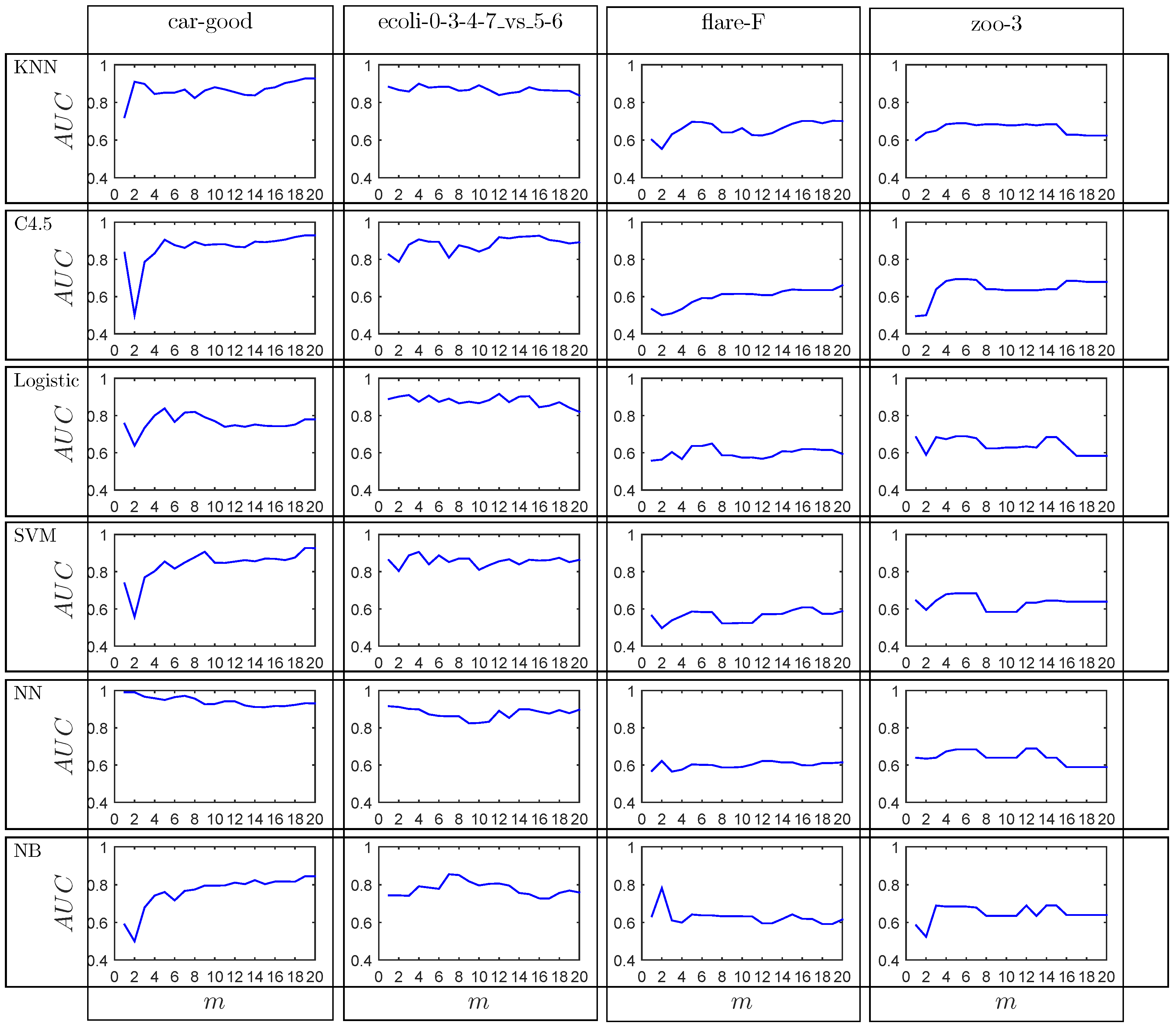
The problem in the algorithm shown in Algorithm 1 is how to set the cluster number m used by partition method for partitioning the majority class. In this section, K-Means was selected as the candidate partition method, and the six conventional classification methods, namely k-nearest neighbor (KNN), C4.5, logistic regression (LR), support vector machine (SVM), neural network (NN) and naive Bayes (NB), were selected as the basic classifiers, in order to evaluate the impact of parameter m on the performance of the proposed method. In addition, AUC was selected as the candidate measurement.
Figure 3 reports the impact of parameter m on the performances of the six learning methods, namely KNN, C4.5, LR, SVM, NN and NB, in term of AUC, where each row indicates the performance of a given classifier on four data sets and the columns are the results of the six classifiers on a given data set. For each sub-figure, the horizontal axis is the value of m growing gradually from 1 to 20 with step 1 and the vertical axis is the average AUC performance on 10-fold cross validation. For example, the sub-figure of the second row (corresponding to algorithm C4.5) and the third column (corresponding to data set flare-F) shows the AUC curve of C4.5 on data set flare-F. Here, the four data sets, namely car-good, ecoli-0-3-4-7_vs_5-6, flare-F and zoo-3, are selected as candidate data sets to evaluate the impact of m. More details about the four data sets refer to Section 5.1. The results are obtained as follows: given the value of m, 10-fold cross validation is conducted on each data set and 10 results are obtained. Then, the final result is calculated by averaging the 10 results, which is drawn as a point in the figure.
From Figure 3, partition methods can effectively improve the performance of models on most data sets ( corresponding to the original model). In addition, we observed from Figure 3 that classifiers achieve acceptable AUC performance if , where and are the size of majority class and minority class, respectively. Take classifier KNN on data set car-good as an example. The AUC is rather good at . Similar results can be observed from other subfigures in Figure 3. This result is not in accordance with the intuitive expectation of , since the partition method can not guarantee that the size of clusters are similar to each other [53]. In fact, our experiments show that the size of some clusters may be much smaller than that of the minority class, which leads to a novel imbalance and thus may reduce the model performance. Therefore, we take in the following experiments.
5. Experiments
5.1. Experimental Setup
This paper focuses only on the binary classification, and seventeen binary class imbalanced data sets, the details of which are shown in Table 2, were randomly selected from the KEEL repository [54], where Instances, Attributes and IR are the size of data sets, number of attributes and imbalance ratio, respectively. The imbalance ratio is defined as the ratio of the size of the majority class to that of the minority class.
To evaluate the performance of the proposed method on class-imbalanced problems, a ten-fold cross-validation strategy was applied: each data set is divided into ten folds with similar sizes, and nine folds are used to train a model. The remaining one is used for testing the model [55]. On each data set, we conducted ten times the ten-fold validation and, therefore, 100 models were actually constructed.
Thirty methods were designed for the experiment, and, based on a basic classifier used by the proposed method (refer to line 6 of Algorithm 1), the methods are grouped into six categories.
KNN Based Methods:
- Data-partition-KNN (DP-KNN) partitions the majority class into m clusters using K-Means and learns a KNN model on each set obtained by merging each cluster and minority class. For prediction, DP-KNN selects a KNN model according to the learned K-Means model to predict the example class. Here, we set (for KNN) , where and represent the size of majority class and that of minority class (refer to Section 4).
- SMOTE-KNN (S-KNN) oversamples the training set using SMOTE to obtain a relatively balanced class distribution, and on which a KNN model is learned. Similar to KNN and DP-KNN, k was set to 3.
- Data-partition-SMOTE-KNN (DPS-KNN) is similar to DP-KNN with the exception that DPS-KNN used both K-Means and SMOTE to preprocess the training set, and we set and .
- MWMOTE-KNN (MWMO-KNN) first oversamples the training set using MWMOTE [14], and, based on that, a KNN model is learned.
C4.5 Based Methods:
- C4.5 is an algorithm used to generate a decision tree developed by Ross Quinlan [58]. Authors of the Weka machine learning software described the C4.5 algorithm as “a landmark decision tree program that is probably the machine learning workhorse most widely used in practice to date” [59]. Here, a pruned C4.5 algorithm was used.
- Data-partition-C4.5 (DP-C4.5) is similar to DP-KNN with the exception that C4.5 was used to learn basic classifiers instead of KNN, and the partition number m was set to be .
- SMOTE-C4.5 (S-C4.5) is similar to S-KNN with the exception that C4.5 instead of KNN was used to train basic models.
- Data-partition-SMOTE-C4.5 (DPS-C4.5) is similar to DPS-KNN with the exception that C4.5 was used to train base models.
- MWMOTE-C4.5 (MWMO-C4.5) first oversamples the training set using MWMOTE [14], and, based on that, a C4.5 model is learned.
Logistic Regression Based Methods:
- Logistic regression (LR) [60] is a regression model where the dependent variable is categorical. In this paper, a binary logistic regression model was used to predict the class label of an example based on the example’s features.
- Data-partition-logistic-regression (DP-LR) is similar to DP-KNN except that DP-LR learns LR models instead of KNN.
- SMOTE-logistic-regression (S-LR) is similar to S-KNN except that S-LR learns LR models instead of KNN.
- Data-partition-SMOTE-logistic-regression (DPS-LR) is similar to DPS-KNN except that DPS-LR learns LR instead of KNN models.
- MWMOTE-LR (MWMO-LR) first oversamples the training set using MWMOTE [14], and, based on that, an LR model is learned.
Support Vector Machine Based Methods:
- Support vector machine [61] (SVM) constructs a hyperplane or set of hyperplanes in a high-dimensional space, which can be used for classification. In the SVM model, a good separation is achieved by the hyperplane that has the largest distance to the nearest training data point of any class.
- Data-partition-SVM (DP-SVM) is similar to DP-KNN with the exception that SVM classification models instead of KNN were learned.
- SMOTE-SVM (S-SVM) is similar to S-KNN with the exception that SVM classification models instead of KNN were learned.
- Data-partition-SMOTE-SVM (DPS-SVM) is similar to DPS-KNN with the exception that SVM models instead of KNN were learned.
- MWMOTE-SVM (MWMO-SVM) first oversamples the training set using MWMOTE [14], and, based on that, an SVM model is learned.
Neural Network Based Methods:
- Neural Network (NN) [62] with one hidden layer was learned and the hidden units were set to be the mean of the input and output number.
- Data-partition-NN (DP-NN) is similar to DP-KNN, except that the NN model was used instead of KNN to train basic classifiers.
- SMOTE-NN (S-NN) is similar to S-KNN except that the NN model was used instead of KNN to train basic classifiers.
- Data-partition-SMOTE-NN (DPS-NN) is similar to DPS-KNN except that the NN model was used instead of KNN to train basic classifiers.
- MWMOTE-NN (MWMO-NN) first oversamples the training set using MWMOTE [14], and, based on that, an NN model is learned.
Naive Bayes Based Methods:
- Naive Bayes (NB) [63] is a simple probabilistic classifier with naive independence assumptions between the features.
- Data-partition-NB (DP-NB) is similar to DP-KNN with the exception that the learning model was NB instead of KNN.
- SMOTE-NB (S-NB) is similar to S-KNN with the exception that the learning model was NB instead of KNN.
- Data-partition-SMOTE-NB (DPS-NB) is similar to DPS-KNN with the exception that the learning model was NB instead of KNN.
- MWMOTE-NB (MWMO-NB) first oversamples the training set using MWMOTE [14], and, based on that, an NB model is learned.
In addition, the parameters of SMOTE used by the above methods, namely S-KNN, DPS-KNN, S-C4.5, DPS-C4.5, S-LR, DPS-LR, S-SVM, DPS-SVM, S-NN, DPS-NN, S-NB and DPS-NB, were set as follows: nearest neighbor number was set to be 5 and the number of generated examples equals the size of the minority class.
5.2. Experimental Results
This section reports the experimental results of the 30 classification methods that are grouped into six categories according to the basic learner used by the proposed method, as introduced in Section 5.1. The corresponding experimental results are shown in five tables, where Table 3, Table 4, Table 5 and Table 6 report the summary results of methods on measures of recall, g-mean, f-measure and AUC, respectively. Table 7 reports the number of data sets on which the proposed method outperforms the compared methods. In Table 3, Table 4, Table 5 and Table 6, the values in parentheses are ranks of methods on the corresponding measures. On each data set, the results of the best performed methods within their categories are shown in bold. The last column of each table shows the average performance of each method on the 17 data sets, and the best average performance are shown in bold. In these tables, the experimental results are separated by blank lines according to different algorithm categories, and the first method (the proposed method) of each category is compared with the other four methods. For simplicity, this subsection names the proposed method as DPS (data-patition and SMOTE based method), and treats DPS compared with the other method m as DPS-m vs. m. For example, DPS compared with KNN means DSP-KNN vs. KNN. The ranks of these methods in these tables are calculated as follows [55,64]: on a given data set, the best performing method gets the rank of 1.0, the second best ranks 2.0, and so on. In case of ties, average ranks are assigned. Table 7 provides the number of data sets on which DPS outperform their compared methods on different measures. For example, the value “15” in the second row and the second column of Table 7 indicates that DPS (DPS-KNN) outperforms KNN on 15 out of 17 data sets on measure of recall.
Table 3 reports the summary results and ranks of the 30 methods on recall. From Table 3, DPS outperforms the other methods on most of the 17 data sets. Specifically, the number of data sets on which DPS outperforms the compared methods on recall are shown in Table 7. The ranks of DPS methods on most of the data sets are much smaller than other methods, and DPS-KNN ranks first with the average rank of 7.0, followed by DPS-NN with average rank of 8.2, DPS-C4.5(8.8), S-NN(9.9), DP-NN(10.4), MWMO-NN(10.9), DPS-LR(11.4), S-KNN(11.7), DP-C4.5(11.7), DPS-SVM(11.8), DP-LR(12.5), DPS-NB(12.5), MWMO-KNN(13.8), NN(14.0), DP-KNN(14.2), S-C4.5(14.8), S-LR(17.0), DP-NB(18.1), S-NB(18.2), MWMO-C4.5(18.3), KNN(18.6), S-SVM(18.8), DP-SVM(19.3), MWMO-LR(19.4), MWMO-NB(19.5), C4.5(20.8), LR(21.8), NB(22.6), MWMO-SVM(22.9) and SVM(26.2). These results indicate that the proposed method works well for class-imbalance problems and it can effectively enhance the performance of traditional methods on identifying minority class examples. Note: DPS can not improve NN (neural network) performance much since NN is a nonlinear classifier that can capture the local information of the data.
Table 4 reports the summary results and the ranks of the 30 methods on g-mean. Similar to the results on recall, Table 4 shows that DPS outperforms the compared methods on most of the 17 data sets, and the number of data sets on which DPS outperforms the compared methods are shown in Table 7. Table 4 also shows that the ranks of DPS methods on most of the data sets are much lower than other methods, and DPS-KNN ranks first with the average rank of 7.0, followed by DPS-NN(9.1), DPS-C4.5(9.2), S-KNN(9.6), DP-NN(10.0), S-NN(10.5), DPS-SVM(11.3), DPS-LR(11.9), DP-C4.5(11.9), DP-KNN(11.9), MWMO-KNN(12.0), MWMO-NN(12.0), NN(12.9), DP-LR(13.4), S-C4.5(13.9), DPS-NB(15.1), KNN(16.1), MWMO-C4.5(17.6), S-SVM(17.8), S-LR(18.2), DP-SVM(18.8), DP-NB(19.5), S-NB(19.8), MWMO-LR(20.2), C4.5(20.4), MWMO-NB(21.1), LR(21.1), MWMO-SVM(22.7), NB(24.0) and SVM(26.1). These results indicate that the proposed method can effectively enhance the performance of traditional methods on both minority class and majority class.
Table 5 summarizes the experimental results and the ranks of the compared methods on f-measure. Similarly, the number of data sets on which DPS outperforms the compared methods on f-measure are shown in Table 7. The ranks of DPS methods on most of the data sets are also much smaller than other methods, and MWMO-KNN ranks first with the average rank of 9.7, followed by DPS-SVM(9.9), S-KNN(9.9), DPS-KNN(10.3), NN(10.7), DP-KNN(11.6), KNN(12.0), DP-NN(12.0), S-NN(12.1), S-C4.5(12.2), MWMO-NN(12.5), DPS-NN(12.8), DPS-C4.5(14.4), DPS-LR(14.9), S-SVM(15.2), S-LR(15.8), MWMO-C4.5(16.1), DP-SVM(16.0), DP-C4.5(16.2), DP-LR(16.5), LR(17.5), MWMO-LR(18.1), C4.5(19.4), DPS-NB(19.6), S-NB(19.8), MWMO-SVM(19.9), MWMO-NB(20.4), DP-NB(21.5), NB(23.8) and SVM(24.3). Comparing the results of Table 5 with those of Table 3 and Table 4, we observe that the performance of DPS on f-measure are not as good as on recall and g-mean, which indicates that DPS incorrectly classifies many majority class examples to be minority ones.
Table 6 depicts experimental results and ranks of compared methods on AUC. Similar to the results above, DPS wins on most of 17 data sets compared to other methods, and the number of data sets on which DPS outperforms the compared methods on AUC are also shown in Table 7. Table 6 shows that the ranks of DPS methods on most of the data sets are also much smaller than other methods, and DPS-KNN ranks first with the average rank of 6.9, DPS-NN(9.1), S-KNN(9.5), DP-NN(10.2), DPS-C4.5(10.3), S-NN(10.7), DPS-SVM(10.9), DP-KNN(11.1), MWMO-KNN(11.2), MWMO-NN(12.3), DPS-LR(12.6), NN(13.1), S-C4.5(13.3), DP-C4.5(13.5), DP-LR(14.0), KNN(15.3), DPS-NB(16.0), S-LR(16.8), S-SVM(17.0), MWMO-C4.5(17.4), DP-SVM(18.6), MWMO-LR(19.9), C4.5(20.1), S-NB(20.3), DP-NB(20.5), LR(20.8), MWMO-NB(21.4), MWMO-SVM(22.1), NB(24.6) and SVM(25.7).
6. Conclusions
This paper proposes a classification method based on data-partitioning and SMOTE for the class-imbalanced problem. In the learning stage, the proposed method partitions the majority class into several clusters, merges each cluster with the minority class as several new sets, and oversamples the new sets to obtain relatively more balanced new training sets. Then, a classification model is learned from each new training set and thus a repository of models is constructed. In the prediction stage, a model is selected from this repository using the partition method learned in the learning stage to predict the class of an example. Experimental results show that the proposed method significantly enhances the performances of conventional methods on class-imbalanced problems, and compared to some other existing classification methods for tackling class-imbalanced problems, the proposed method also shows superiority in terms of recall, g-mean, f-measure and AUC.
In this paper, although we limited the analyses to two-class imbalanced problems and only used K-means and SMOTE as the partitioning and sampling technique, respectively, the general ideas derived in this paper are valid for broad multi-class imbalanced problems. Future work will involve further testing the performance of the proposed method on multi-class problems, automating the selection of the parameters of K-means. In addition, many partition methods and sampling techniques can be used for the proposed methods, and therefore it will be also important to study the impact of other partitioning methods and sampling techniques on the proposed method.
Author Contributions
H.G. initiated the research, J.Z. wrote the paper, C.-A.W. supervised the research work and provided helpful suggestions.
Funding
This work is supported in part by the National Natural Science Foundation of China (No. 61602422, 61572417), in part by the Project of the Science and Technology Department of Henan Province (No. 182102210132), in part by the National Natural Science Foundation of Henan (No. 182300410145), in part by Innovation Team Support Plan of University Science and Technology of Henan Province (No. 19IRTSTHN014), in part by Nanhu Scholars Program for Young Scholars of XYNU, and in part by the Scientific Research Foundation of Graduate School of Xinyang Normal University (No. 2017KYJJ13).
Conflicts of Interest
The authors declare no conflict of interest.
References
- Guo, H.; Li, Y.; Shang, J.; Mingyun, G.; Yuanyue, H.; Bing, G. Learning from class-imbalanced data: Review of methods and applications. Expert Syst. Appl. 2017, 73, 220–239. [Google Scholar] [CrossRef]
- Galar, M.; Fernández, A.; Tartas, E.B.; Sola, H.B.; Herrera, F. A Review on Ensembles for the Class Imbalance Problem: Bagging-, Boosting-, and Hybrid-Based Approaches. IEEE Trans. Syst. Man Cybern. Part C 2012, 42, 463–484. [Google Scholar] [CrossRef]
- Sanz, J.A.; Bernardo, D.; Herrera, F.; Bustince, H.; Hagras, H. A Compact Evolutionary Interval-Valued Fuzzy Rule-Based Classification System for the Modeling and Prediction of Real-World Financial Applications With Imbalanced Data. IEEE Trans. Fuzzy Syst. 2015, 23, 973–990. [Google Scholar] [CrossRef] [Green Version]
- López, V.; Fernández, A.; García, S.; Palade, V.; Herrera, F. An insight into classification with imbalanced data: Empirical results and current trends on using data intrinsic characteristics. Inf. Sci. 2013, 250, 113–141. [Google Scholar] [CrossRef]
- Chawla, N.V.; Japkowicz, N.; Kotcz, A. Editorial: Special issue on learning from imbalanced data sets. SIGKDD Explor. 2004, 6, 1–6. [Google Scholar] [CrossRef]
- Beyan, C.; Fisher, R.B. Classifying imbalanced data sets using similarity based hierarchical decomposition. Pattern Recognit. 2015, 48, 1653–1672. [Google Scholar] [CrossRef] [Green Version]
- Batista, G.E.A.P.A.; Prati, R.C.; Monard, M.C. A study of the behavior of several methods for balancing machine learning training data. SIGKDD Explor. 2004, 6, 20–29. [Google Scholar] [CrossRef]
- Liu, X.; Wu, J.; Zhou, Z. Exploratory Undersampling for Class-Imbalance Learning. IEEE Trans. Syst. Man Cybern. Part B Cybern. 2009, 39, 539–550. [Google Scholar] [CrossRef] [Green Version]
- Tahir, M.A.; Kittler, J.; Mikolajczyk, K.; Yan, F. A Multiple Expert Approach to the Class Imbalance Problem Using Inverse Random under Sampling. In Lecture Notes in Computer Science, Proceedings of the 8th International Workshop on Multiple Classifier Systems (MCS), Reykjavik, Iceland, 10–12 June 2009; Benediktsson, J.A., Kittler, J., Roli, F., Eds.; Springer: Berlin/Heidelberg, Germany, 2009; Volume 5519, pp. 82–91. [Google Scholar] [CrossRef] [Green Version]
- Chawla, N.V.; Bowyer, K.W.; Hall, L.O.; Kegelmeyer, W.P. SMOTE: Synthetic Minority Over-sampling Technique. J. Artif. Intell. Res. 2002, 16, 321–357. [Google Scholar] [CrossRef]
- Li, P.; Qiao, P.; Liu, Y. A Hybrid Re-sampling Method for SVM Learning from Imbalanced Data Sets. In Proceedings of the Fifth International Conference on Fuzzy Systems and Knowledge Discovery (FSKD), Jinan, China, 18–20 October 2008; Ma, J., Yin, Y., Yu, J., Zhou, S., Eds.; IEEE Computer Society: Washington, DC, USA, 2008; Volume 2, pp. 65–69. [Google Scholar] [CrossRef]
- Sobhani, P.; Viktor, H.; Matwin, S. Learning from Imbalanced Data Using Ensemble Methods and Cluster-Based Undersampling. In Proceedings of the Third International Workshop on New Frontiers in Mining Complex Patterns (NFMCP), Nancy, France, 19 September 2014; pp. 69–83. [Google Scholar] [CrossRef]
- Yen, S.; Lee, Y. Cluster-based under-sampling approaches for imbalanced data distributions. Expert Syst. Appl. 2009, 36, 5718–5727. [Google Scholar] [CrossRef]
- Barua, S.; Islam, M.M.; Yao, X.; Murase, K. MWMOTE-Majority Weighted Minority Oversampling Technique for Imbalanced Data Set Learning. IEEE Trans. Knowl. Data Eng. 2014, 26, 405–425. [Google Scholar] [CrossRef]
- Bhowan, U.; Johnston, M.; Zhang, M.; Yao, X. Evolving diverse ensembles using genetic programming for classification with unbalanced data. IEEE Trans. Evol. Comput. 2013, 17, 368–386. [Google Scholar] [CrossRef]
- Wang, S.; Yao, X. Multiclass imbalance problems: Analysis and potential solutions. IEEE Trans. Syst. Man Cybern. Part B Cybern. 2012, 42, 1119–1130. [Google Scholar] [CrossRef] [PubMed]
- Zhang, Y.D.; Zhang, Y.; Phillips, P.; Dong, Z.; Wang, S. Synthetic minority oversampling technique and fractal dimension for identifying multiple sclerosis. Fractals 2017, 25, 1740010. [Google Scholar] [CrossRef]
- Zhang, Y.; Fu, P.; Liu, W.; Chen, G. Imbalanced data classification based on scaling kernel-based support vector machine. Neural Comput. Appl. 2014, 25, 927–935. [Google Scholar] [CrossRef]
- Guo, H.; Liu, H.; Wu, C.; Zhi, W.; Xiao, Y.; She, W. Logistic discrimination based on G-mean and F-measure for imbalanced problem. J. Intell. Fuzzy Syst. 2016, 31, 1155–1166. [Google Scholar] [CrossRef]
- Zhang, Q.; Yang, L.T.; Chen, Z.; Li, P. PPHOPCM: Privacy-preserving high-order possibilistic c-means algorithm for big data clustering with cloud computing. IEEE Trans. Big Data 2017. [Google Scholar] [CrossRef]
- Napierała, K.; Stefanowski, J.; Wilk, S. Learning from imbalanced data in presence of noisy and borderline examples. In Proceedings of the International Conference on Rough Sets and Current Trends in Computing, Warsaw, Poland, 28–30 June 2010; Springer: Berlin/Heidelberg, Germany, 2010; pp. 158–167. [Google Scholar]
- Weiss, G.M.; Provost, F.J. Learning When Training Data are Costly: The Effect of Class Distribution on Tree Induction. J. Artif. Intell. Res. 2003, 19, 315–354. [Google Scholar] [CrossRef]
- Japkowicz, N.; Stephen, S. The class imbalance problem: A systematic study. Intell. Data Anal. 2002, 6, 429–449. [Google Scholar]
- Lin, W.; Tsai, C.; Hu, Y.; Jhang, J. Clustering-based undersampling in class-imbalanced data. Inf. Sci. 2017, 409, 17–26. [Google Scholar] [CrossRef]
- Sun, Y.; Wong, A.K.C.; Kamel, M.S. Classification of Imbalanced Data: A Review. Int. J. Pattern Recognit. Artif. Intell. 2009, 23, 687–719. [Google Scholar] [CrossRef]
- Wang, S.; Minku, L.L.; Yao, X. Resampling-Based Ensemble Methods for Online Class Imbalance Learning. IEEE Trans. Knowl. Data Eng. 2015, 27, 1356–1368. [Google Scholar] [CrossRef]
- Lin, M.; Tang, K.; Yao, X. Dynamic sampling approach to training neural networks for multiclass imbalance classification. IEEE Trans. Neural Netw. Learn. Syst. 2013, 24, 647–660. [Google Scholar] [PubMed]
- Branco, P.; Torgo, L.; Ribeiro, R.P. A Survey of Predictive Modelling under Imbalanced Distributions. arXiv, 2015; arXiv:1505.01658. [Google Scholar]
- Zhai, J.; Zhai, M.; Kang, X. Condensed fuzzy nearest neighbor methods based on fuzzy rough set technique. Intell. Data Anal. 2014, 18, 429–447. [Google Scholar] [CrossRef]
- Devi, D.; Biswas, S.K.; Purkayastha, B. Redundancy-driven modified Tomek-link based undersampling: A solution to class imbalance. Pattern Recognit. Lett. 2017, 93, 3–12. [Google Scholar] [CrossRef]
- Nguyen, H.M.; Cooper, E.W.; Kamei, K. Borderline over-sampling for imbalanced data classification. Int. J. Knowl. Eng. Soft Data Paradig. 2011, 3, 4–21. [Google Scholar] [CrossRef]
- Han, H.; Wang, W.; Mao, B. Borderline-SMOTE: A New Over-Sampling Method in Imbalanced Data Sets Learning. In Lecture Notes in Computer Science, Proceedings of the International Conference on Intelligent Computing on Advances in Intelligent Computing (ICIC 2005), Hefei, China, 23–26 August 2005; Huang, D., Zhang, X., Huang, G., Eds.; Springer: Berlin/Heidelberg, Germany, 2005; Volume 3644, pp. 878–887. [Google Scholar] [CrossRef]
- Bunkhumpornpat, C.; Sinapiromsaran, K.; Lursinsap, C. Safe-Level-SMOTE: Safe-Level-Synthetic Minority Over-Sampling TEchnique for Handling the Class Imbalanced Problem. In Lecture Notes in Computer Science, Proceedings of the 13th Pacific-Asia Conference on Advances in Knowledge Discovery and Data Mining (PAKDD 2009), Bangkok, Thailand, 27–30 April 2009; Theeramunkong, T., Kijsirikul, B., Cercone, N., Ho, T.B., Eds.; Springer: Berlin/Heidelberg, Germany, 2009; Volume 5476, pp. 475–482. [Google Scholar] [CrossRef]
- Prachuabsupakij, W.; Soonthornphisaj, N. Clustering and combined sampling approaches for multi-class imbalanced data classification. In Advances in Information Technology and Industry Applications; Springer: Berlin/Heidelberg, Germany, 2012; pp. 717–724. [Google Scholar]
- Zhang, Q.; Zhu, C.; Yang, L.T.; Chen, Z.; Zhao, L.; Li, P. An Incremental CFS Algorithm for Clustering Large Data in Industrial Internet of Things. IEEE Trans. Ind. Inform. 2017, 13, 1193–1201. [Google Scholar] [CrossRef]
- Macqueen, J. Some Methods for Classification and Analysis of MultiVariate Observations. In Proceedings of the Berkeley Symposium on Mathematical Statistics and Probability; University of California Press: Berkeley, CA, USA, 1967; pp. 281–297. [Google Scholar]
- Sampath, S.; Ramya, B. Rough ISODATA Algorithm. Int. J. Fuzzy Syst. Appl. 2013, 3, 1–14. [Google Scholar] [CrossRef]
- Kaufman, L.; Rousseeuw, P.J. Finding Groups in Data: An Introduction to Cluster Analysis; John Wiley: Hoboken, NJ, USA, 1990. [Google Scholar]
- Xu, R.; Wunsch, D. Survey of clustering algorithms. IEEE Trans. Neural Netw. 2005, 16, 645–678. [Google Scholar] [CrossRef] [PubMed]
- Wu, D.; Chen, X.; Chen, C.; Zhang, J.; Xiang, Y.; Zhou, W. On Addressing the Imbalance Problem: A Correlated KNN Approach for Network Traffic Classification. In Lecture Notes in Computer Science, Proceedings of the 8th International Conference on Network and System Security (NSS 2014), Xi’an, China, 15–17 October 2014; Au, M.H., Carminati, B., Kuo, C.J., Eds.; Springer: Berlin/Heidelberg, Germany, 2014; Volume 8792, pp. 138–151. [Google Scholar] [CrossRef]
- Mennicke, J.; Münzenmayer, C.; Schmid, U. Classifier Learning for Imbalanced Data—A Comparison of kNN, SVM, and Decision Tree Learning; VDM: Saarbrücken, Germany, 2008. [Google Scholar]
- Brumen, B.; Rozman, I.; Hericko, M.; Cernezel, A.; Hölbl, M. Best-Fit Learning Curve Model for the C4.5 Algorithm. Informatica 2014, 25, 385–399. [Google Scholar] [CrossRef]
- Albisua, I.; Arbelaitz, O.; Gurrutxaga, I.; Muguerza, J.; Pérez, J.M. C4.5 Consolidation Process: An Alternative to Intelligent Oversampling Methods in Class Imbalance Problems. In Lecture Notes in Computer Science, Proceedings of the 14th Conference of the Spanish Association for Artificial Intelligence Advances in Artificial Intelligence (CAEPIA 2011), La Laguna, Spain, 7–11 November 2011; Lozano, J.A., Gámez, J.A., Moreno, J.A., Eds.; Springer: Berlin/Heidelberg, Germany, 2011; Volume 7023, pp. 74–83. [Google Scholar] [CrossRef]
- Guo, H.; Zhi, W.; Liu, H.; Xu, M. Imbalanced Learning Based on Logistic Discrimination. Comp. Int. Neurosci. 2016, 2016, 1–10. [Google Scholar] [CrossRef] [PubMed]
- Xu, G.; Hu, B.; Príncipe, J.C. Robust bounded logistic regression in the class imbalance problem. In Proceedings of the 2016 International Joint Conference on Neural Networks (IJCNN 2016), Vancouver, BC, Canada, 24–29 July 2016; pp. 1434–1441. [Google Scholar] [CrossRef]
- Zhang, C.; Guo, J.; Lu, J. Research on Classification Method of High-Dimensional Class-Imbalanced Data Sets Based on SVM. In Proceedings of the Second IEEE International Conference on Data Science in Cyberspace (DSC 2017), Shenzhen, China, 26–29 June 2017; pp. 60–67. [Google Scholar] [CrossRef]
- Yan, Q.; Xia, S.; Meng, F. Optimizing Cost-Sensitive SVM for Imbalanced Data: Connecting Cluster to Classification. arXiv, 2017; arXiv:1702.01504. [Google Scholar]
- Wang, S.; Liu, W.; Wu, J.; Cao, L.; Meng, Q.; Kennedy, P.J. Training deep neural networks on imbalanced data sets. In Proceedings of the 2016 International Joint Conference on Neural Networks (IJCNN 2016), Vancouver, BC, Canada, 24–29 July 2016; pp. 4368–4374. [Google Scholar] [CrossRef]
- Dorado-Moreno, M.; Pérez-Ortiz, M.; Gutiérrez, P.A.; Ciria, R.; Briceño, J.; Hervás-Martínez, C. Dynamically weighted evolutionary ordinal neural network for solving an imbalanced liver transplantation problem. Artif. Intell. Med. 2017, 77, 1–11. [Google Scholar] [CrossRef] [PubMed]
- Zhang, Q.; Yang, L.T.; Chen, Z.; Li, P. A survey on deep learning for big data. Inf. Fusion 2018, 42, 146–157. [Google Scholar] [CrossRef]
- Swezey, R.M.E.; Shiramatsu, S.; Ozono, T.; Shintani, T. An Improvement for Naive Bayes Text Classification Applied to Online Imbalanced Crowdsourced Corpuses. In Modern Advances in Intelligent Systems and Tools; Studies in Computational Intelligence; Ding, W., Jiang, H., Ali, M., Li, M., Eds.; Springer: Berlin/Heidelberg, Germany, 2012; Volume 431, pp. 147–152. [Google Scholar] [CrossRef]
- Hang, Y.; Fong, S.; Wong, R.K.; Sun, G. Optimizing Classification Decision Trees by Using Weighted Naïve Bayes Predictors to Reduce the Imbalanced Class Problem in Wireless Sensor Network. Int. J. Distrib. Sens. Netw. 2013, 9, 460641. [Google Scholar] [CrossRef]
- Da Cunha Rodrigues, C.M. Predictive Modeling using Railway Event Alarms System. arXiv, 2015; arXiv:1106.4557. [Google Scholar]
- Alcalá-Fdez, J.; Fernández, A.; Luengo, J.; Derrac, J.; García, S. KEEL Data-Mining Software Tool: Data Set Repository, Integration of Algorithms and Experimental Analysis Framework. Multiple-Valued Log. Soft Comput. 2011, 17, 255–287. [Google Scholar]
- Demsar, J. Statistical Comparisons of Classifiers over Multiple Data Sets. J. Mach. Learn. Res. 2006, 7, 1–30. [Google Scholar]
- Altman, N.S. An Introduction to Kernel and Nearest-Neighbor Nonparametric Regression. Am. Stat. 1992, 46, 175–185. [Google Scholar] [Green Version]
- Wu, X.; Yang, J.; Wang, S. Tea category identification based on optimal wavelet entropy and weighted k-Nearest Neighbors algorithm. Multimed. Tools Appl. 2018, 77, 3745–3759. [Google Scholar] [CrossRef]
- Quinlan, J.R. C4.5: Programs for Machine Learning; Morgan Kaufmann: Burlington, MA, USA, 1993. [Google Scholar]
- Witten, L.H.; Frank, E.; Hall, M.A. Data Mining: Practical Machine Learning Tools and Techniques, 3rd ed.; ACM Sigmod Record: New York, NY, USA, 2011; Volume 31, pp. 76–77. [Google Scholar]
- Seal, H.L. Estimation of the probability of an event as a function of several independent variables. Biometrika 1967, 54, 167–179. [Google Scholar]
- Cortes, C.; Vapnik, V. Support-Vector Networks. Mach. Learn. 1995, 20, 273–297. [Google Scholar] [CrossRef]
- Schmidhuber, J. Deep learning in neural networks: An overview. Neural Netw. 2015, 61, 85–117. [Google Scholar] [CrossRef] [PubMed] [Green Version]
- Webb, G.I.; Boughton, J.R.; Wang, Z. Not So Naive Bayes: Aggregating One-Dependence Estimators. Mach. Learn. 2005, 58, 5–24. [Google Scholar] [CrossRef] [Green Version]
- García, S.; Fernández, A.; Luengo, J.; Herrera, F. Advanced nonparametric tests for multiple comparisons in the design of experiments in computational intelligence and data mining: Experimental analysis of power. Inf. Sci. 2010, 180, 2044–2064. [Google Scholar] [CrossRef]
Figure 1.
Characteristics of data. (Left): original data; (Center): after partition; (Right): after merging and over-sampling. The bars represent the majority class samples, the crosses represent the minority class samples, and the hollow cross represents the sample generated by oversampling.
Figure 1.
Characteristics of data. (Left): original data; (Center): after partition; (Right): after merging and over-sampling. The bars represent the majority class samples, the crosses represent the minority class samples, and the hollow cross represents the sample generated by oversampling.

Figure 2.
Diagram of the proposed method.

Figure 3.
Impact of parameter m on the performance of models.


Table 1.
Confusion matrix of biclass problem.
| Predicted as Positive | Predicted as Negative | |
|---|---|---|
| Actually Positive | True Positives (TP) | False Negatives (FN) |
| Actually Negative | False Positives (FP) | True Negatives (TN) |
Table 2.
Summary description of imbalanced data sets.
| ID | Data Set | Instances | Attributes | IR (Imbalance Ratio) |
|---|---|---|---|---|
| id1 | segment0 | 2308 | 19 | 6.02 |
| id2 | yeast-0-3-5-9_vs_7-8 | 506 | 8 | 9.12 |
| id3 | yeast-0-2-5-6_vs_3-7-8-9 | 1004 | 8 | 9.14 |
| id4 | ecoli-0-4-6_vs_5 | 203 | 6 | 9.15 |
| id5 | ecoli-0-3-4-7_vs_5-6 | 257 | 7 | 9.28 |
| id6 | ecoli-0-1-4-7_vs_2-3-5-6 | 336 | 7 | 10.59 |
| id7 | led7digit-0-2-4-5-6-7-8-9_vs_1 | 443 | 7 | 10.97 |
| id8 | glass-0-6_vs_5 | 108 | 9 | 11.00 |
| id9 | glass-0-1-4-6_vs_2 | 205 | 9 | 11.06 |
| id10 | ecoli-0-1-4-7_vs_5-6 | 332 | 6 | 12.28 |
| id11 | shuttle-c0-vs-c4 | 1829 | 9 | 13.87 |
| id12 | page-blocks-1-3_vs_4 | 472 | 10 | 15.86 |
| id13 | zoo-3 | 101 | 16 | 19.20 |
| id14 | shuttle-6_vs_2-3 | 230 | 9 | 22.00 |
| id15 | flare-F | 1066 | 11 | 23.79 |
| id16 | car-good | 1728 | 6 | 24.04 |
| id17 | poker-9_vs_7 | 244 | 10 | 29.50 |
Table 3.
Experimental results of models on Recall.
| Algorithm | ID1 | ID2 | ID3 | ID4 | ID5 | ID6 | ID7 | ID8 | ID9 |
|---|---|---|---|---|---|---|---|---|---|
| DPS-KNN | 0.9955(4.0) | 0.5600(4.0) | 0.6213(6.0) | 0.8450(4.5) | 0.8200(4.0) | 0.8183(1.0) | 0.8525(2.0) | 0.7600(17.0) | 0.4400(7.0) |
| KNN | 0.9875(10.0) | 0.4220(10.0) | 0.5560(12.0) | 0.8450(4.5) | 0.7450(21.0) | 0.7333(14.0) | 0.8008(20.0) | 0.6000(26.0) | 0.1250(24.0) |
| DP-KNN | 0.9939(6.0) | 0.4360(9.0) | 0.5598(11.0) | 0.8250(8.0) | 0.7550(19.0) | 0.7567(8.0) | 0.8592(1.0) | 0.6600(22.5) | 0.2650(19.0) |
| S-KNN | 0.9924(8.0) | 0.5120(5.0) | 0.6271(5.0) | 0.8500(2.0) | 0.7950(11.0) | 0.8017(2.0) | 0.8333(5.5) | 0.7300(19.0) | 0.2000(21.0) |
| MWMO-KNN | 0.9897(9.0) | 0.4660(6.5) | 0.5864(8.0) | 0.8450(4.5) | 0.7667(17.0) | 0.7583(7.0) | 0.8058(17.0) | 0.7500(18.0) | 0.2050(20.0) |
| DPS-C4.5 | 0.9830(15.0) | 0.3940(12.0) | 0.5239(16.0) | 0.8100(11.0) | 0.7933(12.0) | 0.7883(3.0) | 0.8283(9.5) | 0.9000(3.0) | 0.3800(10.0) |
| C4.5 | 0.9669(26.0) | 0.2040(28.0) | 0.3759(24.0) | 0.5800(28.0) | 0.5917(27.0) | 0.6550(22.0) | 0.7642(26.0) | 0.9000(3.0) | 0.3100(16.5) |
| DP-C4.5 | 0.9772(20.5) | 0.2600(20.0) | 0.3971(23.0) | 0.8200(9.5) | 0.7917(13.0) | 0.7417(11.0) | 0.8283(9.5) | 0.9000(3.0) | 0.2700(18.0) |
| S-C4.5 | 0.9854(11.0) | 0.3660(13.0) | 0.4978(18.0) | 0.6950(24.5) | 0.7500(20.0) | 0.69671(6.0) | 0.7942(22.0) | 0.9000(3.0) | 0.5000(5.0) |
| MWMO-C4.5 | 0.9781(19.0) | 0.2940(17.0) | 0.4698(21.0) | 0.6300(26.0) | 0.6333(26.0) | 0.6517(23.0) | 0.7692(25.0) | 0.9000(3.0) | 0.3700(11.0) |
| DPS-LR | 0.9589(27.0) | 0.4660(6.5) | 0.5530(13.0) | 0.8450(4.5) | 0.8600(2.0) | 0.7633(6.0) | 0.8342(4.0) | 0.8200(12.0) | 0.4250(8.0) |
| LR | 0.9678(25.0) | 0.1940(29.0) | 0.4144(22.0) | 0.7500(21.5) | 0.7833(14.0) | 0.6700(21.0) | 0.8017(18.5) | 0.8100(13.0) | 0.0100(27.0) |
| DP-LR | 0.9151(28.0) | 0.3620(14.0) | 0.3491(26.0) | 0.8300(7.0) | 0.8833(1.0) | 0.7767(4.0) | 0.8333(5.5) | 0.8300(10.0) | 0.3500(12.0) |
| S-LR | 0.6192(30.0) | 0.2620(19.0) | 0.5742(10.0) | 0.7750(19.0) | 0.8083(7.5) | 0.7383(12.5) | 0.8225(13.0) | 0.6100(25.0) | 0.3400(14.0) |
| MWMO-LR | 0.7942(29.0) | 0.2520(21.0) | 0.5309(15.0) | 0.7650(20.0) | 0.7600(18.0) | 0.6750(20.0) | 0.7967(21.0) | 0.7800(14.5) | 0.1850(22.0) |
| DPS-SVM | 0.9842(14.0) | 0.4060(11.0) | 0.5799(9.0) | 0.8600(1.0) | 0.8033(9.0) | 0.7500(9.5) | 0.8283(9.5) | 0.7800(14.5) | 0.1300(23.0) |
| SVM | 0.9803(18.0) | 0.2200(24.5) | 0.1157(30.0) | 0.6950(24.5) | 0.6400(25.0) | 0.2300(30.0) | 0.7925(23.0) | 0.0000(30.0) | 0.0000(29.0) |
| DP-SVM | 0.9818(16.0) | 0.1880(30.0) | 0.2163(29.0) | 0.8050(12.0) | 0.7117(22.0) | 0.5717(27.0) | 0.8283(9.5) | 0.7100(20.0) | 0.0300(25.0) |
| S-SVM | 0.9848(12.0) | 0.2200(24.5) | 0.6043(7.0) | 0.7950(14.0) | 0.8283(3.0) | 0.6933(17.5) | 0.8250(12.0) | 0.1900(28.0) | 0.0000(29.0) |
| MWMO-SVM | 0.9845(13.0) | 0.2200(24.5) | 0.3690(25.0) | 0.7500(21.5) | 0.6683(24.0) | 0.5333(29.0) | 0.8017(18.5) | 0.1700(29.0) | 0.0000(29.0) |
| DPS-NN | 0.9964(2.0) | 0.5840(3.0) | 0.7784(3.0) | 0.7900(16.0) | 0.8000(10.0) | 0.7500(9.5) | 0.8358(3.0) | 0.8600(6.5) | 0.6200(2.0) |
| NN | 0.9936(7.0) | 0.3380(15.0) | 0.5518(14.0) | 0.8000(13.0) | 0.8183(5.0) | 0.6883(19.0) | 0.8192(15.5) | 0.8400(8.0) | 0.0200(26.0) |
| DP-NN | 0.9961(3.0) | 0.4460(8.0) | 0.6489(4.0) | 0.7850(18.0) | 0.7783(15.0) | 0.7233(15.0) | 0.8308(7.0) | 0.8600(6.5) | 0.5500(4.0) |
| S-NN | 0.9988(1.0) | 0.6680(1.0) | 0.9293(1.0) | 0.7900(16.0) | 0.8117(6.0) | 0.7383(12.5) | 0.8200(14.0) | 0.8300(10.0) | 0.7350(1.0) |
| MWMO-NN | 0.9951(5.0) | 0.5980(2.0) | 0.8086(2.0) | 0.7900(16.0) | 0.8083(7.5) | 0.6933(17.5) | 0.8192(15.5) | 0.8300(10.0) | 0.5850(3.0) |
| DPS-NB | 0.9811(17.0) | 0.3260(16.0) | 0.3091(28.0) | 0.8200(9.5) | 0.7733(16.0) | 0.7683(5.0) | 0.7575(27.0) | 0.7700(16.0) | 0.3400(14.0) |
| NB | 0.9748(22.0) | 0.2180(27.0) | 0.5066(17.0) | 0.4400(30.0) | 0.5017(30.0) | 0.5550(28.0) | 0.7525(28.0) | 0.4100(27.0) | 0.3400(14.0) |
| DP-NB | 0.9741(23.0) | 0.2760(18.0) | 0.3161(27.0) | 0.6250(27.0) | 0.5583(28.0) | 0.6400(25.0) | 0.7742(24.0) | 0.6800(21.0) | 0.3100(16.5) |
| S-NB | 0.9772(20.5) | 0.2200(24.5) | 0.4946(19.0) | 0.7300(23.0) | 0.7050(23.0) | 0.6450(24.0) | 0.7258(29.0) | 0.6600(22.5) | 0.4950(6.0) |
| MWMO-NB | 0.9687(24.0) | 0.2380(22.0) | 0.4818(20.0) | 0.4450(29.0) | 0.5167(29.0) | 0.5750(26.0) | 0.6817(30.0) | 0.6300(24.0) | 0.4150(9.0) |
| algorithm | id10 | id11 | id12 | id13 | id14 | id15 | id16 | id17 | AVE |
| DPS-KNN | 0.8433(1.0) | 0.9944(11.0) | 0.9617(12.0) | 0.3200(9.5) | 0.8400(25.5) | 0.5325(4.0) | 0.9705(4.0) | 0.6500(2.5) | 0.7544(7.0) |
| KNN | 0.7683(17.5) | 0.9911(22.5) | 0.9417(15.0) | 0.2900(17.0) | 0.9000(16.5) | 0.1345(27.0) | 0.3410(24.0) | 0.5000(15.0) | 0.6283(18.6) |
| DP-KNN | 0.7683(17.5) | 0.9919(17.0) | 0.9367(16.0) | 0.3200(9.5) | 0.7200(28.0) | 0.3525(8.5) | 0.8438(9.0) | 0.5600(10.0) | 0.6826(14.2) |
| S-KNN | 0.8233(4.0) | 0.9911(22.5) | 0.9717(7.0) | 0.3000(14.5) | 0.9100(12.5) | 0.2180(17.0) | 0.5421(21.0) | 0.6500(2.5) | 0.6910(11.7) |
| MWMO-KNN | 0.7817(13.5) | 0.9919(17.0) | 0.9633(11.0) | 0.3000(14.5) | 0.9400(8.0) | 0.2100(18.0) | 0.5374(22.0) | 0.6300(5.0) | 0.6871(13.8) |
| DPS-C4.5 | 0.8200(5.0) | 1.0000(4.5) | 0.9833(5.5) | 0.3800(1.5) | 0.9300(10.0) | 0.3525(8.5) | 0.9195(6.0) | 0.6200(6.5) | 0.7298(8.8) |
| C4.5 | 0.6217(26.0) | 1.0000(4.5) | 0.9933(1.5) | 0.0000(30.0) | 1.0000(3.0) | 0.0020(30.0) | 0.0000(30.0) | 0.0300(29.0) | 0.5291(20.8) |
| DP-C4.5 | 0.8067(8.0) | 1.0000(4.5) | 0.9833(5.5) | 0.3800(1.5) | 0.9300(10.0) | 0.1710(20.0) | 0.7807(11.0) | 0.5900(8.0) | 0.6840(11.7) |
| S-C4.5 | 0.7083(22.0) | 1.0000(4.5) | 0.9933(1.5) | 0.3000(14.5) | 1.0000(3.0) | 0.1430(26.0) | 0.7502(13.0) | 0.1600(22.0) | 0.6612(14.8) |
| MWMO-C4.5 | 0.6417(25.0) | 1.0000(4.5) | 0.9433(14.0) | 0.1300(28.0) | 1.0000(3.0) | 0.0805(28.0) | 0.7238(14.0) | 0.2100(20.5) | 0.6133(18.3) |
| DPS-LR | 0.8183(6.0) | 0.9853(26.0) | 0.9483(13.0) | 0.3200(9.5) | 0.8400(25.5) | 0.3510(10.0) | 0.7081(15.0) | 0.5400(12.5) | 0.7080(11.4) |
| LR | 0.7633(19.0) | 0.7231(30.0) | 0.5717(26.0) | 0.2000(26.5) | 0.9900(6.0) | 0.1575(24.0) | 0.2788(27.0) | 0.1100(25.0) | 0.5409(21.8) |
| DP-LR | 0.8300(3.0) | 0.9846(27.0) | 0.9317(17.0) | 0.3300(6.5) | 0.8600(24.0) | 0.2580(14.0) | 0.6476(16.0) | 0.6200(6.5) | 0.6818(12.5) |
| S-LR | 0.8333(2.0) | 0.7507(29.0) | 0.7100(21.0) | 0.2100(23.0) | 0.8900(21.0) | 0.2415(15.0) | 0.5671(19.0) | 0.2100(20.5) | 0.5860(17.0) |
| MWMO-LR | 0.7817(13.5) | 0.7561(28.0) | 0.6283(23.0) | 0.2200(20.0) | 0.9000(16.5) | 0.2015(19.0) | 0.4986(23.0) | 0.2300(19.0) | 0.5783(19.4) |
| DPS-SVM | 0.8083(7.0) | 0.9887(25.0) | 0.8600(20.0) | 0.3400(4.0) | 0.8800(23.0) | 0.3205(11.0) | 0.9240(5.0) | 0.6500(2.5) | 0.6996(11.8) |
| SVM | 0.5250(28.0) | 0.9919(17.0) | 0.4200(30.0) | 0.2100(23.0) | 0.7000(30.0) | 0.0190(29.0) | 0.0960(28.0) | 0.0000(30.0) | 0.3903(26.2) |
| DP-SVM | 0.7150(21.0) | 0.9895(24.0) | 0.6433(22.0) | 0.3400(4.0) | 0.7800(27.0) | 0.1630(21.0) | 0.7510(12.0) | 0.5700(9.0) | 0.5879(19.3) |
| S-SVM | 0.7900(10.0) | 0.9919(17.0) | 0.4233(29.0) | 0.2100(23.0) | 0.8900(21.0) | 0.1580(23.0) | 0.5452(20.0) | 0.0700(28.0) | 0.5423(18.8) |
| MWMO-SVM | 0.6683(23.0) | 0.9919(17.0) | 0.4350(28.0) | 0.2100(23.0) | 0.9000(16.5) | 0.1540(25.0) | 0.6074(27.0) | 0.1000(26.5) | 0.5037(22.9) |
| DPS-NN | 0.7933(9.0) | 0.9919(17.0) | 0.9850(4.0) | 0.3200(9.5) | 0.9100(12.5) | 0.4730(5.0) | 0.9157(7.0) | 0.5500(11.0) | 0.7620(8.2) |
| NN | 0.7700(16.0) | 0.9919(17.0) | 0.9667(3.0) | 0.3000(6.5) | 0.9000(21.0) | 0.1585(12.0) | 1.0000(8.0) | 0.4000(12.5) | 0.6680(10.4) |
| DP-NN | 0.7867(11.0) | 0.9919(17.0) | 0.9917(3.0) | 0.3300(6.5) | 0.8900(21.0) | 0.3025(12.0) | 0.8983(8.0) | 0.5400(12.5) | 0.7264(10.4) |
| S-NN | 0.7833(12.0) | 0.9919(17.0) | 0.9667(9.0) | 0.2300(18.5) | 0.9000(16.5) | 0.4220(6.0) | 0.9926(2.0) | 0.2800(17.5) | 0.7581(9.9) |
| MWMO-NN | 0.7783(15.0) | 0.9928(12.0) | 0.9667(9.0) | 0.2300(18.5) | 0.9000(16.5) | 0.2755(13.0) | 0.9724(3.0) | 0.2800(17.5) | 0.7249(10.9) |
| DPS-NB | 0.7383(20.0) | 0.9992(9.5) | 0.9283(18.5) | 0.3400(4.0) | 1.0000(3.0) | 0.3775(7.0) | 0.8000(10.0) | 0.6500(2.5) | 0.6870(12.5) |
| NB | 0.4833(30.0) | 1.0000(4.5) | 0.5667(27.0) | 0.1000(29.0) | 0.7100(29.0) | 0.6290(3.0) | 0.0074(29.0) | 0.1000(26.5) | 0.4879(22.6) |
| DP-NB | 0.5567(27.0) | 0.9992(9.5) | 0.9283(18.5) | 0.3100(12.0) | 1.0000(3.0) | 0.2265(16.0) | 0.5940(18.0) | 0.5200(14.0) | 0.6052(18.1) |
| S-NB | 0.6517(24.0) | 1.0000(4.5) | 0.5950(25.0) | 0.2100(23.0) | 0.9300(10.0) | 0.6770(1.0) | 0.2960(26.0) | 0.1500(23.0) | 0.5978(18.2) |
| MWMO-NB | 0.5083(29.0) | 1.0000(4.5) | 0.5967(24.0) | 0.2000(26.5) | 0.9800(7.0) | 0.6465(2.0) | 0.3100(25.0) | 0.1400(24.0) | 0.5490(19.5) |
Table 4.
Experimental results of models on g-mean.
| Algorithm | ID1 | ID2 | ID3 | ID4 | ID5 | ID6 | ID7 | ID8 | ID9 |
|---|---|---|---|---|---|---|---|---|---|
| DPS-KNN | 0.9964(2.0) | 0.6876(1.0) | 0.7533(3.0) | 0.8936(5.0) | 0.8764(6.0) | 0.8769(1.0) | 0.8905(4.0) | 0.7474(17.0) | 0.4837(6.0) |
| KNN | 0.9923(10.0) | 0.5950(10.0) | 0.7266(8.0) | 0.9067(2.0) | 0.8361(17.0) | 0.8261(11.0) | 0.8743(19.0) | 0.5953(25.0) | 0.1606(23.0) |
| DP-KNN | 0.9959(3.0) | 0.6093(7.0) | 0.7278(7.0) | 0.8772(7.0) | 0.8353(18.0) | 0.8406(6.0) | 0.9000(1.0) | 0.6505(23.0) | 0.3008(19.0) |
| S-KNN | 0.9941(8.0) | 0.6553(4.0) | 0.7628(1.0) | 0.9080(1.0) | 0.8691(8.0) | 0.8650(2.0) | 0.8907(2.0) | 0.7238(19.0) | 0.2492(20.0) |
| MWMO-KNN | 0.9929(9.0) | 0.6292(6.0) | 0.7385(4.0) | 0.9061(3.0) | 0.8517(14.0) | 0.8415(5.0) | 0.8776(17.0) | 0.7443(18.0) | 0.2434(21.0) |
| DPS-C4.5 | 0.9887(17.0) | 0.5576(12.0) | 0.6826(15.0) | 0.8526(15.0) | 0.8417(16.0) | 0.8521(3.0) | 0.8865(12.0) | 0.8844(4.0) | 0.4255(9.0) |
| C4.5 | 0.9813(21.0) | 0.3501(29.0) | 0.5926(23.0) | 0.6726(28.0) | 0.6913(27.0) | 0.7713(22.0) | 0.8448(25.0) | 0.8949(2.5) | 0.3702(14.0) |
| DP-C4.5 | 0.9859(19.0) | 0.4279(18.0) | 0.5989(22.0) | 0.8583(13.0) | 0.8501(15.0) | 0.8295(8.0) | 0.8876(9.0) | 0.8839(5.0) | 0.3069(17.0) |
| S-C4.5 | 0.9909(14.0) | 0.5492(13.0) | 0.6805(16.0) | 0.7491(25.0) | 0.8153(21.0) | 0.7873(19.0) | 0.8669(22.0) | 0.8949(2.5) | 0.5587(4.0) |
| MWMO-C4.5 | 0.9870(18.0) | 0.4544(17.0) | 0.6598(19.0) | 0.7086(26.0) | 0.7174(26.0) | 0.7594(23.0) | 0.8519(24.0) | 0.8954(1.0) | 0.4222(10.0) |
| DPS-LR | 0.9704(22.0) | 0.6021(8.0) | 0.6934(12.0) | 0.8865(6.0) | 0.8891(2.0) | 0.8267(10.0) | 0.8888(8.0) | 0.8132(12.0) | 0.4585(8.0) |
| LR | 0.9820(20.0) | 0.3519(28.0) | 0.6267(20.0) | 0.8228(22.0) | 0.8544(12.0) | 0.7793(20.0) | 0.8771(18.0) | 0.7934(13.0) | 0.0092(27.0) |
| DP-LR | 0.9513(24.0) | 0.5367(14.0) | 0.5572(24.0) | 0.8731(8.0) | 0.9024(1.0) | 0.8439(4.0) | 0.8840(16.0) | 0.8222(11.0) | 0.3910(11.0) |
| S-LR | 0.7803(30.0) | 0.4246(20.0) | 0.7362(5.0) | 0.8329(19.0) | 0.8621(10.0) | 0.8271(9.0) | 0.8875(10.0) | 0.5940(26.0) | 0.3846(12.0) |
| MWMO-LR | 0.8801(29.0) | 0.4129(21.0) | 0.7076(11.0) | 0.8289(20.0) | 0.8272(20.0) | 0.7767(21.0) | 0.8730(21.0) | 0.7599(15.0) | 0.2072(22.0) |
| DPS-SVM | 0.9911(13.0) | 0.5647(11.0) | 0.7186(10.0) | 0.9021(4.0) | 0.8664(9.0) | 0.8376(7.0) | 0.8894(7.0) | 0.7747(14.0) | 0.1522(24.0) |
| SVM | 0.9895(16.0) | 0.3795(25.0) | 0.2841(30.0) | 0.7858(24.0) | 0.7580(25.0) | 0.3294(30.0) | 0.8643(23.0) | 0.0000(30.0) | 0.0000(29.0) |
| DP-SVM | 0.9900(15.0) | 0.3482(30.0) | 0.4180(29.0) | 0.8619(11.0) | 0.8027(22.0) | 0.6996(26.0) | 0.8906(3.0) | 0.7057(20.0) | 0.0339(25.0) |
| S-SVM | 0.9918(11.0) | 0.3795(25.0) | 0.7586(2.0) | 0.8589(12.0) | 0.8885(3.0) | 0.8016(16.0) | 0.8869(11.0) | 0.1900(28.0) | 0.0000(29.0) |
| MWMO-SVM | 0.9916(12.0) | 0.3821(23.0) | 0.5427(25.0) | 0.8288(21.0) | 0.7685(24.0) | 0.6332(29.0) | 0.8736(20.0) | 0.1700(29.0) | 0.0000(29.0) |
| DPS-NN | 0.9953(6.0) | 0.6742(2.0) | 0.6699(18.0) | 0.8459(18.0) | 0.8619(11.0) | 0.8251(12.0) | 0.8902(5.0) | 0.8536(7.0) | 0.6290(2.0) |
| NN | 0.9955(4.5) | 0.5132(15.0) | 0.7217(9.0) | 0.8628(10.0) | 0.8835(4.0) | 0.7961(18.0) | 0.8844(14.0) | 0.8354(8.0) | 0.0232(26.0) |
| DP-NN | 0.9955(4.5) | 0.5975(9.0) | 0.7330(6.0) | 0.8477(17.0) | 0.8527(13.0) | 0.8082(15.0) | 0.8899(6.0) | 0.8542(6.0) | 0.5758(3.0) |
| S-NN | 0.9971(1.0) | 0.6633(3.0) | 0.4760(28.0) | 0.8557(14.0) | 0.8806(5.0) | 0.8249(13.0) | 0.8847(13.0) | 0.8243(10.0) | 0.6872(1.0) |
| MWMO-NN | 0.9950(7.0) | 0.6306(5.0) | 0.6030(21.0) | 0.8522(16.0) | 0.8741(7.0) | 0.7976(17.0) | 0.8843(15.0) | 0.8259(9.0) | 0.5482(5.0) |
| DPS-NB | 0.9493(25.0) | 0.4809(16.0) | 0.5258(27.0) | 0.8643(9.0) | 0.8351(19.0) | 0.8097(14.0) | 0.8335(27.0) | 0.7537(16.0) | 0.3468(15.0) |
| NB | 0.9242(27.0) | 0.3751(27.0) | 0.6915(13.0) | 0.5413(30.0) | 0.6044(30.0) | 0.6592(28.0) | 0.8088(28.0) | 0.4100(27.0) | 0.3047(18.0) |
| DP-NB | 0.9628(23.0) | 0.4259(19.0) | 0.5296(26.0) | 0.7025(27.0) | 0.6465(28.0) | 0.7189(25.0) | 0.8418(26.0) | 0.6679(21.0) | 0.3145(16.0) |
| S-NB | 0.9038(28.0) | 0.3795(25.0) | 0.6829(14.0) | 0.8030(23.0) | 0.7969(23.0) | 0.7505(24.0) | 0.7954(29.0) | 0.6595(22.0) | 0.4762(7.0) |
| MWMO-NB | 0.9320(26.0) | 0.4009(22.0) | 0.6714(17.0) | 0.5567(29.0) | 0.6064(29.0) | 0.6939(27.0) | 0.7750(30.0) | 0.6290(24.0) | 0.3818(13.0) |
| algorithm | id10 | id11 | id12 | id13 | id14 | id15 | id16 | id17 | AVE |
| DPS-KNN | 0.8878(1.0) | 0.9971(11.0) | 0.9768(11.5) | 0.3132(11.0) | 0.8391(25.0) | 0.6782(4.0) | 0.9058(8.0) | 0.6465(2.0) | 0.7912(7.0) |
| KNN | 0.8428(17.0) | 0.9955(22.5) | 0.9666(13.0) | 0.2894(17.0) | 0.9000(14.5) | 0.2482(27.0) | 0.5499(24.0) | 0.5000(14.0) | 0.6944(16.1) |
| DP-KNN | 0.8380(18.0) | 0.9959(15.0) | 0.9628(16.0) | 0.3139(10.0) | 0.7193(28.0) | 0.5343(8.0) | 0.8794(9.0) | 0.5591(8.0) | 0.7377(11.9) |
| S-KNN | 0.8744(5.0) | 0.9955(22.5) | 0.9837(5.0) | 0.2971(14.0) | 0.9100(12.5) | 0.3642(17.0) | 0.7089(21.0) | 0.6493(1.0) | 0.7471(9.6) |
| MWMO-KNN | 0.8499(15.0) | 0.9959(15.0) | 0.9793(9.0) | 0.2965(15.0) | 0.9400(8.0) | 0.3380(19.0) | 0.7076(22.0) | 0.6291(4.0) | 0.7389(12.0) |
| DPS-C4.5 | 0.8712(6.0) | 1.0000(3.0) | 0.9777(10.0) | 0.3727(1.5) | 0.9238(10.0) | 0.5125(10.0) | 0.9303(7.0) | 0.5804(6.0) | 0.7729(9.2) |
| C4.5 | 0.7243(26.0) | 0.9997(7.0) | 0.9935(1.5) | 0.0000(30.0) | 0.9977(1.0) | 0.0044(30.0) | 0.0000(30.0) | 0.0296(29.0) | 0.5834(20.4) |
| DP-C4.5 | 0.8658(8.0) | 1.0000(3.0) | 0.9768(11.5) | 0.3727(1.5) | 0.9231(11.0) | 0.2907(20.0) | 0.8522(12.0) | 0.5569(9.0) | 0.7334(11.9) |
| S-C4.5 | 0.8055(21.0) | 1.0000(3.0) | 0.9935(1.5) | 0.3000(13.0) | 0.9975(2.5) | 0.2596(26.0) | 0.8540(11.0) | 0.1581(22.0) | 0.7212(13.9) |
| MWMO-C4.5 | 0.7589(24.0) | 1.0000(3.0) | 0.9638(15.0) | 0.1300(28.0) | 0.9975(2.5) | 0.1442(28.0) | 0.8251(14.0) | 0.2083(21.0) | 0.6755(17.6) |
| DPS-LR | 0.8796(3.0) | 0.9924(26.0) | 0.9639(14.0) | 0.3154(9.0) | 0.8389(26.0) | 0.5134(9.0) | 0.8153(15.0) | 0.5297(13.0) | 0.7575(11.9) |
| LR | 0.8485(16.0) | 0.8448(30.0) | 0.7023(26.0) | 0.1983(26.0) | 0.9870(6.0) | 0.2768(23.0) | 0.4776(27.0) | 0.1100(25.0) | 0.6201(21.1) |
| DP-LR | 0.8755(4.0) | 0.9921(27.0) | 0.9494(17.0) | 0.3220(7.0) | 0.8568(24.0) | 0.4041(14.0) | 0.7784(16.0) | 0.6107(5.0) | 0.7383(13.4) |
| S-LR | 0.8921(19.0) | 0.8575(28.0) | 0.7996(21.0) | 0.2071(24.0) | 0.8888(22.0) | 0.4030(15.0) | 0.7304(19.0) | 0.2087(20.0) | 0.6657(18.2) |
| MWMO-LR | 0.8578(13.0) | 0.8561(29.0) | 0.7474(23.0) | 0.2182(20.0) | 0.8972(19.0) | 0.3422(18.0) | 0.6758(23.0) | 0.2287(19.0) | 0.6528(20.2) |
| DPS-SVM | 0.8831(2.0) | 0.9942(25.0) | 0.8971(20.0) | 0.3360(3.5) | 0.8793(23.0) | 0.4895(11.0) | 0.9386(5.0) | 0.6441(3.0) | 0.7505(11.3) |
| SVM | 0.6652(27.0) | 0.9959(15.0) | 0.5599(30.0) | 0.2077(22.0) | 0.7000(30.0) | 0.0385(29.0) | 0.2035(28.0) | 0.0000(30.0) | 0.4566(26.1) |
| DP-SVM | 0.8182(20.0) | 0.9946(24.0) | 0.7605(22.0) | 0.3360(3.5) | 0.7793(27.0) | 0.2789(22.0) | 0.8415(13.0) | 0.5661(7.0) | 0.6545(18.8) |
| S-SVM | 0.8710(7.0) | 0.9958(18.5) | 0.5617(29.0) | 0.2077(22.0) | 0.8900(20.5) | 0.2827(21.0) | 0.7112(20.0) | 0.0700(28.0) | 0.6086(17.8) |
| MWMO-SVM | 0.7653(23.0) | 0.9958(18.5) | 0.5695(28.0) | 0.2077(22.0) | 0.9000(14.5) | 0.2715(25.0) | 0.7540(17.0) | 0.1000(26.0) | 0.5738(22.7) |
| DPS-NN | 0.8604(11.0) | 0.9957(20.0) | 0.9884(4.0) | 0.3172(8.0) | 0.9100(12.5) | 0.6184(5.0) | 0.9439(4.0) | 0.5450(10.0) | 0.7897(9.1) |
| NN | 0.8552(14.0) | 0.9959(15.0) | 0.9802(6.5) | 0.2954(16.0) | 0.8989(17.5) | 0.2726(24.0) | 0.9994(1.0) | 0.4000(16.0) | 0.7184(12.9) |
| DP-NN | 0.8617(10.0) | 0.9956(21.0) | 0.9925(3.0) | 0.3255(6.0) | 0.8900(20.5) | 0.4697(12.0) | 0.9359(6.0) | 0.5361(12.0) | 0.7742(10.0) |
| S-NN | 0.8625(9.0) | 0.9959(15.0) | 0.9802(6.5) | 0.2260(18.0) | 0.8991(16.0) | 0.5732(6.0) | 0.9949(2.0) | 0.2778(18.0) | 0.7590(10.5) |
| MWMO-NN | 0.8586(12.0) | 0.9963(12.0) | 0.9800(8.0) | 0.2248(19.0) | 0.8989(17.5) | 0.4306(13.0) | 0.9804(3.0) | 0.2789(17.0) | 0.7447(12.0) |
| DPS-NB | 0.8000(22.0) | 0.9981(10.0) | 0.9333(19.0) | 0.3343(5.0) | 0.9914(5.0) | 0.5439(7.0) | 0.8681(10.0) | 0.5435(11.0) | 0.7301(15.1) |
| NB | 0.5903(30.0) | 0.9999(6.0) | 0.6844(27.0) | 0.0977(29.0) | 0.7088(29.0) | 0.7489(3.0) | 0.0192(29.0) | 0.0963(27.0) | 0.5450(24.0) |
| DP-NB | 0.6425(28.0) | 0.9983(9.0) | 0.9342(18.0) | 0.3066(12.0) | 0.9937(4.0) | 0.3725(16.0) | 0.7481(18.0) | 0.4765(15.0) | 0.6637(19.5) |
| S-NB | 0.7444(25.0) | 0.9996(8.0) | 0.7065(24.0) | 0.2050(25.0) | 0.9295(9.0) | 0.7744(1.0) | 0.4920(26.0) | 0.1406(23.0) | 0.6612(19.8) |
| MWMO-NB | 0.6277(29.0) | 1.0000(3.0) | 0.7055(25.0) | 0.1941(27.0) | 0.9800(7.0) | 0.7621(2.0) | 0.5171(25.0) | 0.1327(24.0) | 0.6215(21.1) |
Table 5.
Experimental results of models on f-measure.
| Algorithm | ID1 | ID2 | ID3 | ID4 | ID5 | ID6 | ID7 | ID8 | ID9 |
|---|---|---|---|---|---|---|---|---|---|
| DPS-KNN | 0.9902(2.0) | 0.4472(4.0) | 0.5497(11.0) | 0.8367(6.0) | 0.7677(10.0) | 0.7983(1.0) | 0.7205(24.0) | 0.6867(17.0) | 0.3148(6.0) |
| KNN | 0.9852(10.0) | 0.4537(2.0) | 0.6157(2.0) | 0.8777(1.0) | 0.7643(11.0) | 0.7681(6.0) | 0.7714(10.0) | 0.5700(25.0) | 0.1273(22.0) |
| DP-KNN | 0.9906(1.0) | 0.4561(1.0) | 0.5971(3.0) | 0.8437(5.0) | 0.7574(15.0) | 0.7846(3.0) | 0.7361(23.0) | 0.6067(24.0) | 0.2210(13.0) |
| S-KNN | 0.9842(11.0) | 0.4469(5.0) | 0.5920(6.0) | 0.8693(3.0) | 0.7789(7.0) | 0.7940(2.0) | 0.7628(16.0) | 0.6900(16.0) | 0.1865(16.0) |
| MWMO-KNN | 0.9835(12.0) | 0.4481(3.0) | 0.5780(7.0) | 0.8737(2.0) | 0.7720(9.0) | 0.7787(5.0) | 0.7743(9.0) | 0.7133(15.0) | 0.1767(17.0) |
| DPS-C4.5 | 0.9757(18.0) | 0.3290(14.0) | 0.4736(18.0) | 0.6939(24.0) | 0.6742(25.0) | 0.6920(21.0) | 0.7552(18.0) | 0.8067(7.0) | 0.2921(8.0) |
| C4.5 | 0.9720(21.0) | 0.2671(30.0) | 0.4813(17.0) | 0.5658(28.0) | 0.6264(27.0) | 0.7059(16.0) | 0.7404(22.0) | 0.8667(2.5) | 0.3120(7.0) |
| DP-C4.5 | 0.9735(20.0) | 0.2729(27.0) | 0.4406(19.0) | 0.7031(23.0) | 0.7151(19.0) | 0.6966(20.0) | 0.7635(14.0) | 0.8033(8.5) | 0.2189(14.0) |
| S-C4.5 | 0.9823(15.0) | 0.3708(7.0) | 0.5395(13.0) | 0.6350(26.0) | 0.7136(20.0) | 0.7000(19.0) | 0.7683(12.0) | 0.8667(2.5) | 0.4328(1.0) |
| MWMO-C4.5 | 0.9775(17.0) | 0.3193(15.0) | 0.5209(15.0) | 0.6213(27.0) | 0.6328(26.0) | 0.6809(23.0) | 0.7539(19.0) | 0.8700(1.0) | 0.3178(5.0) |
| DPS-LR | 0.9303(22.0) | 0.3544(11.0) | 0.4404(20.0) | 0.7957(10.0) | 0.7731(8.0) | 0.7048(17.0) | 0.7491(21.0) | 0.7783(12.0) | 0.2842(10.0) |
| LR | 0.9737(19.0) | 0.2807(26.0) | 0.5297(14.0) | 0.7713(19.0) | 0.7915(6.0) | 0.7264(10.0) | 0.7894(1.0) | 0.7197(14.0) | 0.0040(27.0) |
| DP-LR | 0.9272(23.0) | 0.3604(10.0) | 0.3851(23.0) | 0.7801(15.0) | 0.7622(12.0) | 0.7227(11.0) | 0.7196(25.0) | 0.7850(11.0) | 0.2415(12.0) |
| S-LR | 0.7429(28.0) | 0.3185(16.0) | 0.5962(4.0) | 0.7597(21.0) | 0.7588(14.0) | 0.7518(7.0) | 0.7869(2.0) | 0.5263(26.0) | 0.2855(9.0) |
| MWMO-LR | 0.8543(25.0) | 0.3144(18.0) | 0.5743(8.0) | 0.7630(20.0) | 0.7122(21.0) | 0.7028(18.0) | 0.7773(5.0) | 0.6657(20.0) | 0.1418(21.0) |
| DPS-SVM | 0.9865(7.0) | 0.3680(8.0) | 0.5017(16.0) | 0.8511(4.0) | 0.8054(2.0) | 0.7796(4.0) | 0.7786(4.0) | 0.7483(13.0) | 0.1037(24.0) |
| SVM | 0.9869(6.0) | 0.3094(21.0) | 0.1849(30.0) | 0.7517(22.0) | 0.7072(23.0) | 0.2973(30.0) | 0.7554(17.0) | 0.0000(30.0) | 0.0000(29.0) |
| DP-SVM | 0.9862(8.0) | 0.2674(29.0) | 0.3048(27.0) | 0.8303(7.0) | 0.7598(13.0) | 0.6534(24.0) | 0.7863(3.0) | 0.6850(18.0) | 0.0300(25.0) |
| S-SVM | 0.9893(3.0) | 0.3094(21.0) | 0.6383(1.0) | 0.8180(8.0) | 0.8490(1.0) | 0.7487(8.0) | 0.7767(6.0) | 0.1900(28.0) | 0.0000(29.0) |
| MWMO-SVM | 0.9888(5.0) | 0.3098(19.0) | 0.4172(22.0) | 0.7870(12.0) | 0.7086(22.0) | 0.5895(27.0) | 0.7629(15.0) | 0.1700(29.0) | 0.0000(29.0) |
| DPS-NN | 0.9815(16.0) | 0.3609(9.0) | 0.2820(28.0) | 0.7724(18.0) | 0.7400(17.0) | 0.7078(15.0) | 0.7535(20.0) | 0.8217(5.0) | 0.3907(2.0) |
| NN | 0.9890(4.0) | 0.3818(6.0) | 0.5940(5.0) | 0.8030(9.0) | 0.7977(4.0) | 0.7185(12.0) | 0.7759(7.0) | 0.8100(6.0) | 0.0150(26.0) |
| DP-NN | 0.9834(13.0) | 0.3541(12.0) | 0.4333(21.0) | 0.7763(17.0) | 0.7418(16.0) | 0.7119(14.0) | 0.7697(11.0) | 0.8250(4.0) | 0.3746(3.0) |
| S-NN | 0.9861(9.0) | 0.3058(24.0) | 0.2244(29.0) | 0.7867(13.0) | 0.8018(3.0) | 0.7304(9.0) | 0.7667(13.0) | 0.7933(10.0) | 0.3586(4.0) |
| MWMO-NN | 0.9831(14.0) | 0.3450(13.0) | 0.3363(26.0) | 0.7893(11.0) | 0.7935(5.0) | 0.7173(13.0) | 0.7752(8.0) | 0.8033(8.5) | 0.2710(11.0) |
| DPS-NB | 0.7980(26.0) | 0.3041(25.0) | 0.3621(25.0) | 0.7826(14.0) | 0.7047(24.0) | 0.5667(28.0) | 0.6815(27.0) | 0.6773(19.0) | 0.1691(18.0) |
| NB | 0.7188(29.0) | 0.3065(23.0) | 0.5665(9.0) | 0.5057(30.0) | 0.5483(29.0) | 0.6103(25.0) | 0.5516(29.0) | 0.4100(27.0) | 0.1109(23.0) |
| DP-NB | 0.8640(24.0) | 0.2715(28.0) | 0.3674(24.0) | 0.6461(25.0) | 0.5684(28.0) | 0.5194(29.0) | 0.6851(26.0) | 0.6090(23.0) | 0.1451(20.0) |
| S-NB | 0.6610(30.0) | 0.3094(21.0) | 0.5562(10.0) | 0.7783(16.0) | 0.7167(18.0) | 0.6835(22.0) | 0.5451(30.0) | 0.6567(21.0) | 0.2048(15.0) |
| MWMO-NB | 0.7505(27.0) | 0.3171(17.0) | 0.5419(12.0) | 0.5203(29.0) | 0.5295(30.0) | 0.6029(26.0) | 0.5587(28.0) | 0.6233(22.0) | 0.1639(19.0) |
| algorithm | id10 | id11 | id12 | id13 | id14 | id15 | id16 | id17 | AVE |
| DPS-KNN | 0.7983(5.0) | 0.9971(7.0) | 0.9527(11.0) | 0.2833(15.0) | 0.8267(24.0) | 0.2985(4.0) | 0.3500(25.0) | 0.6000(3.0) | 0.6599(10.3) |
| KNN | 0.7796(10.0) | 0.9954(17.0) | 0.9556(8.0) | 0.2867(12.0) | 0.9000(11.5) | 0.1622(27.0) | 0.4150(23.0) | 0.5000(7.0) | 0.6428(12.0) |
| DP-KNN | 0.7689(14.0) | 0.9958(12.0) | 0.9399(12.0) | 0.2850(13.5) | 0.7100(28.0) | 0.2715(7.0) | 0.4761(18.0) | 0.5467(5.0) | 0.6463(11.6) |
| S-KNN | 0.8070(4.0) | 0.9954(17.0) | 0.9746(1.0) | 0.2850(13.5) | 0.9100(9.5) | 0.2038(19.0) | 0.4534(22.0) | 0.6400(1.0) | 0.6691(9.9) |
| MWMO-KNN | 0.7774(11.0) | 0.9958(12.0) | 0.9698(2.0) | 0.2817(16.0) | 0.9400(6.0) | 0.2044(18.0) | 0.4679(19.0) | 0.6183(2.0) | 0.6679(9.7) |
| DPS-C4.5 | 0.6746(22.0) | 1.0000(1.5) | 0.8354(15.0) | 0.3383(1.5) | 0.8490(22.0) | 0.2739(6.0) | 0.5782(10.0) | 0.2849(14.0) | 0.6192(14.4) |
| C4.5 | 0.6411(26.0) | 0.9962(8.5) | 0.9654(3.5) | 0.0000(30.0) | 0.9667(2.0) | 0.0025(30.0) | 0.0000(30.0) | 0.0250(29.0) | 0.5373(19.4) |
| DP-C4.5 | 0.6899(21.0) | 1.0000(1.5) | 0.8264(16.0) | 0.3383(1.5) | 0.8430(23.0) | 0.1793(23.0) | 0.5285(12.0) | 0.2971(13.0) | 0.6053(16.2) |
| S-C4.5 | 0.6903(20.0) | 0.9996(4.0) | 0.9654(3.5) | 0.3000(8.0) | 0.9650(3.5) | 0.1695(25.0) | 0.7233(6.0) | 0.1317(22.0) | 0.6443(12.2) |
| MWMO-C4.5 | 0.6692(23.0) | 0.9996(4.0) | 0.9176(13.0) | 0.1300(28.0) | 0.9650(3.5) | 0.1057(28.0) | 0.6556(7.0) | 0.1883(20.0) | 0.6074(16.1) |
| DPS-LR | 0.7678(15.0) | 0.9915(24.0) | 0.8760(14.0) | 0.2950(9.0) | 0.8233(25.0) | 0.2422(11.0) | 0.5140(13.0) | 0.4199(11.0) | 0.6318(14.9) |
| LR | 0.7887(8.0) | 0.8287(29.0) | 0.6122(24.0) | 0.1917(25.0) | 0.9483(5.0) | 0.2012(20.0) | 0.3206(27.0) | 0.1100(23.0) | 0.5640(17.5) |
| DP-LR | 0.7473(18.0) | 0.9908(25.0) | 0.8077(17.0) | 0.2907(11.0) | 0.8173(26.0) | 0.2147(17.0) | 0.5018(16.0) | 0.4957(8.0) | 0.6206(16.5) |
| S-LR | 0.8208(3.0) | 0.8443(28.0) | 0.6675(22.0) | 0.1950(24.0) | 0.8750(19.0) | 0.2595(10.0) | 0.4942(17.0) | 0.1900(19.0) | 0.5808(15.8) |
| MWMO-LR | 0.7825(9.0) | 0.7786(30.0) | 0.6315(23.0) | 0.2117(18.0) | 0.8673(21.0) | 0.2415(12.0) | 0.4571(21.0) | 0.2117(18.0) | 0.5699(18.1) |
| DPS-SVM | 0.8247(2.0) | 0.9937(21.0) | 0.7890(18.0) | 0.3183(3.5) | 0.8700(20.0) | 0.2599(9.0) | 0.6544(8.0) | 0.5700(4.0) | 0.6590(9.9) |
| SVM | 0.6154(27.0) | 0.9958(12.0) | 0.5170(28.0) | 0.1967(22.0) | 0.7000(29.0) | 0.0221(29.0) | 0.1437(28.0) | 0.0000(30.0) | 0.4226(24.3) |
| DP-SVM | 0.7907(7.0) | 0.9941(20.0) | 0.6828(21.0) | 0.3183(3.5) | 0.7700(27.0) | 0.1719(24.0) | 0.6040(9.0) | 0.5133(6.0) | 0.5970(16.0) |
| S-SVM | 0.8269(1.0) | 0.9954(17.0) | 0.5117(30.0) | 0.1967(22.0) | 0.8900(14.5) | 0.1972(22.0) | 0.4639(20.0) | 0.0700(27.0) | 0.5571(15.2) |
| MWMO-SVM | 0.7183(19.0) | 0.9954(17.0) | 0.5156(29.0) | 0.1967(22.0) | 0.9000(11.5) | 0.1977(21.0) | 0.5119(14.0) | 0.1000(24.0) | 0.5217(19.9) |
| DPS-NN | 0.7508(17.0) | 0.9935(22.0) | 0.9553(9.0) | 0.3033(6.5) | 0.9100(9.5) | 0.2607(8.0) | 0.7505(5.0) | 0.4817(10.0) | 0.6598(12.8) |
| NN | 0.7767(12.0) | 0.9958(12.0) | 0.9589(5.0) | 0.2750(17.0) | 0.8833(17.5) | 0.1687(26.0) | 0.9866(1.0) | 0.4000(12.0) | 0.6665(10.7) |
| DP-NN | 0.7599(16.0) | 0.9927(23.0) | 0.9588(6.0) | 0.3033(6.5) | 0.8900(14.5) | 0.2345(14.0) | 0.7618(4.0) | 0.4850(9.0) | 0.6680(12.0) |
| S-NN | 0.7919(6.0) | 0.9958(12.0) | 0.9586(7.0) | 0.2083(19.0) | 0.8867(16.0) | 0.2374(13.0) | 0.9713(2.0) | 0.2500(16.0) | 0.6502(12.1) |
| MWMO-NN | 0.7741(13.0) | 0.9962(8.5) | 0.9551(10.0) | 0.2040(20.0) | 0.8833(17.5) | 0.2205(16.0) | 0.8841(3.0) | 0.2633(15.0) | 0.6467(12.5) |
| DPS-NB | 0.6414(25.0) | 0.9808(27.0) | 0.7504(20.0) | 0.3083(5.0) | 0.8930(13.0) | 0.2823(5.0) | 0.5430(11.0) | 0.1639(21.0) | 0.5653(19.6) |
| NB | 0.5303(30.0) | 0.9985(6.0) | 0.5326(27.0) | 0.0883(29.0) | 0.6950(30.0) | 0.3925(1.0) | 0.0129(29.0) | 0.0573(28.0) | 0.4492(23.8) |
| DP-NB | 0.5432(29.0) | 0.9833(26.0) | 0.7582(19.0) | 0.2917(10.0) | 0.9213(8.0) | 0.2305(15.0) | 0.5075(15.0) | 0.2124(17.0) | 0.5367(21.5) |
| S-NB | 0.6674(24.0) | 0.9954(17.0) | 0.5512(25.0) | 0.1833(26.0) | 0.9250(7.0) | 0.3718(3.0) | 0.3314(26.0) | 0.0725(26.0) | 0.5417(19.8) |
| MWMO-NB | 0.5563(28.0) | 0.9996(4.0) | 0.5508(26.0) | 0.1763(27.0) | 0.9800(1.0) | 0.3920(2.0) | 0.3525(24.0) | 0.0778(25.0) | 0.5114(20.4) |
Table 6.
Experimental results of models on AUC.
| Algorithm | ID1 | ID2 | ID3 | ID4 | ID5 | ID6 | ID7 | ID8 | ID9 |
|---|---|---|---|---|---|---|---|---|---|
| DPS-KNN | 0.9965(2.0) | 0.7295(1.0) | 0.7762(3.0) | 0.9143(5.0) | 0.8930(7.0) | 0.8990(1.0) | 0.9026(2.0) | 0.8637(18.0) | 0.6623(6.0) |
| KNN | 0.9923(10.0) | 0.6916(6.0) | 0.7657(6.0) | 0.9198(3.0) | 0.8628(19.0) | 0.8608(9.0) | 0.8890(19.0) | 0.7909(25.0) | 0.5507(21.0) |
| DP-KNN | 0.9959(3.0) | 0.6948(5.0) | 0.7637(7.0) | 0.9081(6.0) | 0.8667(17.0) | 0.8723(3.0) | 0.9076(1.0) | 0.8153(23.0) | 0.6008(13.0) |
| S-KNN | 0.9942(8.0) | 0.7162(2.0) | 0.7875(1.0) | 0.9206(2.0) | 0.8843(10.0) | 0.8922(2.0) | 0.9010(4.0) | 0.8554(19.0) | 0.5689(18.0) |
| MWMO-KNN | 0.9929(9.0) | 0.7020(3.0) | 0.7700(4.0) | 0.9192(4.0) | 0.8719(15.0) | 0.8720(4.0) | 0.8913(18.0) | 0.8679(15.0) | 0.5745(16.0) |
| DPS-C4.5 | 0.9888(17.0) | 0.6431(15.0) | 0.7264(16.0) | 0.8749(19.0) | 0.8671(16.0) | 0.8709(5.0) | 0.8972(12.0) | 0.9344(4.0) | 0.6455(9.0) |
| C4.5 | 0.9816(21.0) | 0.5915(29.0) | 0.6807(22.0) | 0.7719(28.0) | 0.7880(27.0) | 0.8208(22.0) | 0.8701(25.0) | 0.9450(2.5) | 0.6356(11.0) |
| DP-C4.5 | 0.9861(19.0) | 0.5986(27.0) | 0.6797(23.0) | 0.8796(17.0) | 0.8741(13.0) | 0.8524(13.0) | 0.8983(11.0) | 0.9339(5.0) | 0.5978(14.0) |
| S-C4.5 | 0.9910(14.0) | 0.6525(12.0) | 0.7319(14.0) | 0.8264(25.0) | 0.8596(21.0) | 0.8377(16.0) | 0.8858(22.0) | 0.9450(2.5) | 0.7234(3.0) |
| MWMO-C4.5 | 0.9871(18.0) | 0.6252(16.0) | 0.7183(18.0) | 0.7997(27.0) | 0.8039(26.0) | 0.8167(23.0) | 0.8739(24.0) | 0.9455(1.0) | 0.6555(7.0) |
| DPS-LR | 0.9708(22.0) | 0.6727(9.0) | 0.7247(17.0) | 0.9071(7.0) | 0.9106(2.0) | 0.8642(8.0) | 0.8990(10.0) | 0.9014(12.0) | 0.6551(8.0) |
| LR | 0.9822(20.0) | 0.5937(28.0) | 0.7011(19.0) | 0.8684(22.0) | 0.8832(11.0) | 0.8306(20.0) | 0.8914(17.0) | 0.8852(13.0) | 0.4915(29.0) |
| DP-LR | 0.9528(24.0) | 0.6486(14.0) | 0.6512(25.0) | 0.8986(9.0) | 0.9176(1.0) | 0.8702(6.0) | 0.8946(16.0) | 0.9049(11.0) | 0.6213(12.0) |
| S-LR | 0.8071(30.0) | 0.6147(18.0) | 0.7688(5.0) | 0.8760(18.0) | 0.8880(9.0) | 0.8607(10.0) | 0.8996(8.0) | 0.7832(26.0) | 0.6450(10.0) |
| MWMO-LR | 0.8946(29.0) | 0.6142(19.0) | 0.7496(10.0) | 0.8729(20.0) | 0.8600(20.0) | 0.8281(21.0) | 0.8875(21.0) | 0.8672(16.0) | 0.5697(17.0) |
| DPS-SVM | 0.9912(13.0) | 0.6619(11.0) | 0.7506(9.0) | 0.9218(1.0) | 0.8935(6.0) | 0.8690(7.0) | 0.9005(6.0) | 0.8824(14.0) | 0.5321(23.0) |
| SVM | 0.9896(16.0) | 0.6067(22.5) | 0.5546(30.0) | 0.8448(24.0) | 0.8157(25.0) | 0.6121(30.0) | 0.8837(23.0) | 0.5000(30.0) | 0.5000(26.0) |
| DP-SVM | 0.9901(15.0) | 0.5886(30.0) | 0.6023(29.0) | 0.8990(8.0) | 0.8519(22.0) | 0.7832(25.0) | 0.9017(3.0) | 0.8484(20.0) | 0.5044(24.0) |
| S-SVM | 0.9919(11.0) | 0.6067(22.5) | 0.7872(2.0) | 0.8925(11.0) | 0.9098(3.0) | 0.8424(15.0) | 0.8994(9.0) | 0.5950(28.0) | 0.5000(26.0) |
| MWMO-SVM | 0.9917(12.0) | 0.6067(22.5) | 0.6733(24.0) | 0.8703(21.0) | 0.8279(24.0) | 0.7631(29.0) | 0.8880(20.0) | 0.5850(29.0) | 0.5000(26.0) |
| DPS-NN | 0.9953(6.0) | 0.7004(4.0) | 0.6835(21.0) | 0.8835(15.0) | 0.8810(12.0) | 0.8600(11.0) | 0.9003(7.0) | 0.9223(7.0) | 0.7451(2.0) |
| NN | 0.9955(4.5) | 0.6506(13.0) | 0.7604(8.0) | 0.8915(12.0) | 0.8977(4.0) | 0.8360(19.0) | 0.8969(13.0) | 0.9155(8.0) | 0.4968(28.0) |
| DP-NN | 0.9955(4.5) | 0.6669(10.0) | 0.7473(11.0) | 0.8818(16.0) | 0.8732(14.0) | 0.8504(14.0) | 0.9007(5.0) | 0.9229(6.0) | 0.7218(4.0) |
| S-NN | 0.9971(1.0) | 0.6821(8.0) | 0.6065(28.0) | 0.8851(14.0) | 0.8946(5.0) | 0.8573(12.0) | 0.8956(15.0) | 0.9094(10.0) | 0.7567(1.0) |
| MWMO-NN | 0.9951(7.0) | 0.6847(7.0) | 0.6889(20.0) | 0.8860(13.0) | 0.8918(8.0) | 0.8375(18.0) | 0.8968(14.0) | 0.9110(9.0) | 0.6735(5.0) |
| DPS-NB | 0.9500(25.0) | 0.6229(17.0) | 0.6344(27.0) | 0.8956(10.0) | 0.8649(18.0) | 0.8376(17.0) | 0.8577(27.0) | 0.8668(17.0) | 0.5669(19.0) |
| NB | 0.9257(27.0) | 0.6057(25.0) | 0.7391(12.0) | 0.7164(30.0) | 0.7435(30.0) | 0.7731(28.0) | 0.8324(28.0) | 0.7050(27.0) | 0.4724(30.0) |
| DP-NB | 0.9630(23.0) | 0.6036(26.0) | 0.6375(26.0) | 0.8041(26.0) | 0.7675(28.0) | 0.7827(26.0) | 0.8649(26.0) | 0.8263(22.0) | 0.5448(22.0) |
| S-NB | 0.9067(28.0) | 0.6067(22.5) | 0.7332(13.0) | 0.8634(23.0) | 0.8417(23.0) | 0.8152(24.0) | 0.8208(29.0) | 0.8285(21.0) | 0.5866(15.0) |
| MWMO-NB | 0.9329(26.0) | 0.6124(20.0) | 0.7265(15.0) | 0.7189(29.0) | 0.7456(29.0) | 0.7774(27.0) | 0.8059(30.0) | 0.8135(24.0) | 0.5550(20.0) |
| algorithm | id10 | id11 | id12 | id13 | id14 | id15 | id16 | id17 | AVE |
| DPS-KNN | 0.9119(1.0) | 0.9972(11.0) | 0.9789(10.0) | 0.6442(11.0) | 0.9191(25.0) | 0.7238(4.0) | 0.9087(8.0) | 0.8199(2.0) | 0.8553(6.9) |
| KNN | 0.8785(16.0) | 0.9955(22.5) | 0.9703(13.0) | 0.6408(14.0) | 0.9500(14.5) | 0.5600(27.0) | 0.6653(24.0) | 0.7500(11.0) | 0.8079(15.3) |
| DP-KNN | 0.8775(17.5) | 0.9960(15.0) | 0.9667(15.0) | 0.6469(9.5) | 0.8591(28.0) | 0.6516(9.0) | 0.8855(9.0) | 0.7785(7.0) | 0.8286(11.1) |
| S-KNN | 0.9048(3.0) | 0.9955(22.5) | 0.9853(5.0) | 0.6419(13.0) | 0.9550(12.5) | 0.5932(18.0) | 0.7532(21.0) | 0.8239(1.0) | 0.8337(9.5) |
| MWMO-KNN | 0.8838(11.0) | 0.9960(15.0) | 0.9811(9.0) | 0.6404(15.0) | 0.9700(8.0) | 0.5926(19.0) | 0.7531(22.0) | 0.8137(4.0) | 0.8290(11.2) |
| DPS-C4.5 | 0.8840(10.0) | 1.0000(3.0) | 0.9786(11.0) | 0.6778(1.5) | 0.9586(10.0) | 0.6520(8.0) | 0.9325(7.0) | 0.7460(12.0) | 0.8399(10.3) |
| C4.5 | 0.8022(26.0) | 0.9997(7.0) | 0.9944(1.5) | 0.5000(30.0) | 0.9977(1.0) | 0.5007(30.0) | 0.5000(30.0) | 0.5133(29.0) | 0.7584(20.1) |
| DP-C4.5 | 0.8801(15.0) | 1.0000(3.0) | 0.9777(12.0) | 0.6778(1.5) | 0.9580(11.0) | 0.5739(20.0) | 0.8655(12.0) | 0.7395(13.0) | 0.8219(13.5) |
| S-C4.5 | 0.8415(22.0) | 1.0000(3.0) | 0.9944(1.5) | 0.6489(8.0) | 0.9975(2.5) | 0.5655(26.0) | 0.8686(11.0) | 0.5690(22.0) | 0.8199(13.3) |
| MWMO-C4.5 | 0.8123(25.0) | 1.0000(3.0) | 0.9679(14.0) | 0.5617(28.0) | 0.9975(2.5) | 0.5377(28.0) | 0.8526(14.0) | 0.5950(21.0) | 0.7971(17.4) |
| DPS-LR | 0.8968(6.0) | 0.9926(26.0) | 0.9666(16.0) | 0.6469(9.5) | 0.9186(26.0) | 0.6448(10.0) | 0.8320(15.0) | 0.7538(10.0) | 0.8328(12.6) |
| LR | 0.8764(19.0) | 0.8615(30.0) | 0.7788(26.0) | 0.5910(24.0) | 0.9920(5.0) | 0.5731(21.0) | 0.6319(27.0) | 0.5516(23.0) | 0.7637(20.8) |
| DP-LR | 0.9000(4.0) | 0.9922(27.0) | 0.9531(17.0) | 0.6421(12.0) | 0.9264(24.0) | 0.6063(15.0) | 0.8041(16.0) | 0.7950(5.0) | 0.8223(14.0) |
| S-LR | 0.9093(2.0) | 0.8753(28.0) | 0.8436(21.0) | 0.5888(25.0) | 0.9436(22.0) | 0.6099(14.0) | 0.7687(19.0) | 0.5952(20.0) | 0.7810(16.8) |
| MWMO-LR | 0.8837(12.0) | 0.8706(29.0) | 0.8045(23.0) | 0.5985(23.0) | 0.9464(19.0) | 0.5935(17.0) | 0.7359(23.0) | 0.6058(19.0) | 0.7754(19.9) |
| DPS-SVM | 0.8993(5.0) | 0.9943(25.0) | 0.9204(20.0) | 0.6583(3.5) | 0.9393(23.0) | 0.6364(11.0) | 0.9426(5.0) | 0.8177(3.0) | 0.8360(10.9) |
| SVM | 0.7600(28.0) | 0.9960(15.0) | 0.7087(30.0) | 0.6007(20.0) | 0.8500(30.0) | 0.5068(29.0) | 0.5464(28.0) | 0.5000(30.0) | 0.6927(25.7) |
| DP-SVM | 0.8569(20.0) | 0.9947(24.0) | 0.8164(22.0) | 0.6583(3.5) | 0.8893(27.0) | 0.5698(24.0) | 0.8601(13.0) | 0.7799(6.0) | 0.7880(18.6) |
| S-SVM | 0.8917(7.0) | 0.9959(18.5) | 0.7091(29.0) | 0.6007(20.0) | 0.9450(20.5) | 0.5726(22.0) | 0.7563(20.0) | 0.5350(25.0) | 0.7666(17.0) |
| MWMO-SVM | 0.8306(23.0) | 0.9959(18.5) | 0.7141(28.0) | 0.6007(20.0) | 0.9500(14.5) | 0.5721(23.0) | 0.7880(17.0) | 0.5500(24.0) | 0.7475(22.1) |
| DPS-NN | 0.8850(9.0) | 0.9958(20.0) | 0.9899(4.0) | 0.6500(7.0) | 0.9550(12.5) | 0.6921(5.0) | 0.9463(4.0) | 0.7671(8.0) | 0.8502(9.1) |
| NN | 0.8775(17.5) | 0.9960(15.0) | 0.9819(6.5) | 0.6357(17.0) | 0.9489(17.5) | 0.5694(25.0) | 0.9994(1.0) | 0.7000(14.0) | 0.8264(13.1) |
| DP-NN | 0.8829(13.0) | 0.9957(21.0) | 0.9931(3.0) | 0.6533(5.0) | 0.9450(20.5) | 0.6272(12.0) | 0.9392(6.0) | 0.7638(9.0) | 0.8448(10.2) |
| S-NN | 0.8851(8.0) | 0.9960(15.0) | 0.9819(6.5) | 0.6018(18.0) | 0.9491(16.0) | 0.6683(6.0) | 0.9952(2.0) | 0.6347(17.0) | 0.8351(10.7) |
| MWMO-NN | 0.8813(14.0) | 0.9964(12.0) | 0.9816(8.0) | 0.5997(22.0) | 0.9489(17.5) | 0.6146(13.0) | 0.9811(3.0) | 0.6330(18.0) | 0.8295(12.3) |
| DPS-NB | 0.8464(21.0) | 0.9981(10.0) | 0.9459(19.0) | 0.6527(6.0) | 0.9916(6.0) | 0.6621(7.0) | 0.8757(10.0) | 0.6874(16.0) | 0.8092(16.0) |
| NB | 0.7368(30.0) | 0.9999(6.0) | 0.7679(27.0) | 0.5301(29.0) | 0.8539(29.0) | 0.7810(3.0) | 0.5034(29.0) | 0.5250(28.0) | 0.7183(24.6) |
| DP-NB | 0.7661(27.0) | 0.9983(9.0) | 0.9468(18.0) | 0.6403(16.0) | 0.9939(4.0) | 0.6010(16.0) | 0.7817(18.0) | 0.6887(15.0) | 0.7771(20.5) |
| S-NB | 0.8187(24.0) | 0.9996(8.0) | 0.7815(25.0) | 0.5684(26.0) | 0.9645(9.0) | 0.7962(1.0) | 0.6396(26.0) | 0.5291(27.0) | 0.7706(20.3) |
| MWMO-NB | 0.7488(29.0) | 1.0000(3.0) | 0.7826(24.0) | 0.5649(27.0) | 0.9900(7.0) | 0.7876(2.0) | 0.6466(25.0) | 0.5340(26.0) | 0.7496(21.4) |
Table 7.
Number of data sets on which DPS methods outperform the compared methods.
| Algorithm | Recall | G-Mean | F-Measure | AUC |
|---|---|---|---|---|
| DPS-KNN | - | - | - | - |
| KNN | 15 | 15 | 9 | 15 |
| DP-KNN | 15 | 14 | 10 | 15 |
| S-KNN | 12 | 12 | 6 | 12 |
| MWMO-KNN | 14 | 11 | 7 | 13 |
| DPS-C4.5 | - | - | - | - |
| C4.5 | 13 | 14 | 11 | 14 |
| DP-C4.5 | 10 | 12 | 9 | 12 |
| S-C4.5 | 12 | 11 | 5 | 9 |
| MWMO-C4.5 | 14 | 14 | 10 | 13 |
| DPS-LR | - | - | - | - |
| LR | 15 | 15 | 10 | 14 |
| DP-LR | 11 | 11 | 13 | 11 |
| S-LR | 14 | 13 | 10 | 13 |
| MWMO-LR | 16 | 15 | 13 | 15 |
| DPS-SVM | - | - | - | - |
| SVM | 16 | 16 | 15 | 16 |
| DP-SVM | 14 | 14 | 14 | 14 |
| S-SVM | 12 | 12 | 11 | 12 |
| MWMO-SVM | 14 | 14 | 14 | 14 |
| DPS-NN | - | - | - | - |
| NN | 13 | 11 | 6 | 11 |
| DP-NN | 13 | 10 | 5 | 11 |
| S-NN | 9 | 10 | 8 | 10 |
| MWMO-NN | 11 | 14 | 8 | 12 |
| DPS-NB | - | - | - | - |
| NB | 13 | 14 | 12 | 14 |
| DP-NB | 12 | 11 | 10 | 10 |
| S-NB | 13 | 13 | 8 | 13 |
| MWMO-NB | 13 | 13 | 11 | 14 |
© 2018 by the authors. Licensee MDPI, Basel, Switzerland. This article is an open access article distributed under the terms and conditions of the Creative Commons Attribution (CC BY) license (http://creativecommons.org/licenses/by/4.0/).
Share and Cite
MDPI and ACS Style
Guo, H.; Zhou, J.; Wu, C.-A. Imbalanced Learning Based on Data-Partition and SMOTE. Information 2018, 9, 238. https://0-doi-org.brum.beds.ac.uk/10.3390/info9090238
AMA Style
Guo H, Zhou J, Wu C-A. Imbalanced Learning Based on Data-Partition and SMOTE. Information. 2018; 9(9):238. https://0-doi-org.brum.beds.ac.uk/10.3390/info9090238
Chicago/Turabian StyleGuo, Huaping, Jun Zhou, and Chang-An Wu. 2018. "Imbalanced Learning Based on Data-Partition and SMOTE" Information 9, no. 9: 238. https://0-doi-org.brum.beds.ac.uk/10.3390/info9090238
Note that from the first issue of 2016, this journal uses article numbers instead of page numbers. See further details here.