Machine Learning Modeling and Run-to-Run Control of an Area-Selective Atomic Layer Deposition Spatial Reactor

Abstract

Semiconducting materials require stringent design specifications that make their fabrication more difficult and prone to flaws that are costly and damaging to their computing and electrical properties. Area-selective atomic layer deposition is a process that addresses concerns associated with design imperfections but requires substantial monitoring to ensure that process regulation is maintained. This work proposes a run-to-run controller with an exponentially weighted moving average method for an area-selective atomic layer deposition rotary reactor by adjusting the rotation speed of the substrate to control the growth per cycle of the wafer, which is calculated through a multiscale model with machine learning integration for pressure field generation and kinetic Monte Carlo simulations to increase computational efficiency. Results indicate that the run-to-run controller was able to bring the process to the setpoint when subjected to moderate pressure and kinetic shift disturbances.

1. Introduction

With the emergence and modernization of high-performance electronics, the availability and feasibility of this technology has transformed the socioeconomic life of people globally. For example, semiconductors are found in a plethora of applications in the vehicular [1], solar cells [2], telecommunications and smart technology [3,4], and the bioelectronics and medical industries [4,5]. However, the fabrication of these electronics requires a surplus of semiconducting materials, which are an integral component for these devices to perform computationally efficient tasks with stronger energy coherence. By correcting various design flaws, including short-channel effects and current leakage [6,7], gate-all-around (GAA) transistor structures have improved the robustness and performance of modern-day technology [8] within nanoscale thicknesses that approach two-dimensional attributes. However, a consequence of this miniaturization of feature sizes generates obstacles for transistor fabrication: efficiency and accuracy.

The preponderance of high-performance semiconducting materials in advanced electronics is a motivation for increasing their supply and improving inefficient manufacturing practices with processes that yield greater semiconductor quantity and have higher accuracy. For example, the aftermath of semiconductor shortages following the COVID-19 pandemic [9,10] and the looming political implications [11] regarding the dependence of national security on semiconductors, led to increased government investment toward the strengthening of semiconductor yield and quality through the development of innovative fabrication processes [12]. These investments have been fruitful for increasing semiconductor supply and quality following the rise of atomic layer deposition (ALD) [13,14], atomic layer etching (ALE) [15,16], and area-selective atomic layer deposition (AS-ALD) [17,18,19] processes, which possess significant roles in the construction of transistors with nanoscale dimensions by precisely depositing or etching monolayers of substrate material in sequential and cyclical procedures. Recently, research has been conducted on achieving film uniformity for AS-ALD methods without requiring post-processing steps such as ALE to ensure self-alignment during the transistor stacking procedure. AS-ALD has been previously experimented through in silico, atomistic-mesoscopic and multiscale computational fluid dynamics (CFD) modeling to study the spatiotemporal behavior of the process in a spatial, rotary reactor configuration [20,21,22]. Although AS-ALD is characterized by a high accuracy deposition rate, such a process requires regulatory monitoring to ensure that quality conformance is maintained, thereby mitigating the risk of semiconductor performance degradation and nonconformance to product criteria.

To ensure process monitoring in short timescale intervals, semiconductor manufacturing industries propose ex situ or offline control referred to as run-to-run (R2R) control [23], which performs controller adjustments after each batch run or in this case, after the completion of one cycle of AS-ALD. For example, Critical Manufacturing uses an integrative manufacturing execution system (MES) to regulate semiconductor manufacturing processes for etching and lithography by adopting run-to-run control algorithms that implement suitable control actions [24]. Past works have established run-to-run control for atomic layer etching (ALE) processes conducted in a stationary plate and spatial sheet-to-sheet reactor configuration [25,26], for plasma-enhanced atomic layer deposition (PEALD) in an inductively coupled plasma (ICP) reactor [27], and for thermal atomic layer deposition (ALD) in a furnace reactor (PEALD) [28]. This work aims to implement R2R controller action on an AS-ALD rotary reactor in an in silico experiment that regulates the output, growth per cycle, of a multiscale computational fluid dynamics (CFD) simulation when perturbed by pressure and kinetic shift disturbances by performing feedback after each cycle of the AS-ALD process. To reduce the computational demand for the highly complex multiscale simulation, machine learning and C programming language are substituted in place of CFD and the kinetic Monte Carlo simulations to facilitate the generation of output data for the R2R controller. This work will first examine the development of the multiscale CFD model in Section 2, the implementation of machine learning to generate pressure field data in place of the CFD simulation is discussed in Section 3, and the integration of the R2R controller is elucidated in Section 4 with the closed-loop simulations presented in Section 5.

2. Multiscale Computational Fluid Dynamics Model

Area-selective atomic layer deposition (AS-ALD) is defined by a three-step, ABC, process comprising inhibition, adsorption, and oxidation steps that perform selective deposition on growth areas of the substrate [29]. However, conducting experiments in laboratory environments is a time-consuming and laborious process that may yield variable results that depend on idealistic operating conditions. Thus, this section of the manuscript will discuss the development of an in silico approach to replicate the experimental laboratory settings by combining atomistic modeling through first principles quantum mechanics simulations to evaluate kinetic parameters inherent to rate-determining reaction pathways, mesoscopic modeling through the stochastic kinetic Monte Carlo (kMC) computations for studying the surface-scale kinetics, and macroscopic computational fluid dynamics (CFD) to evaluate the mass transfer of reagent and byproduct species in the fluid phase. The conjunction of such simulations constitutes a multiscale model that performs simulations through multiple time and length scales, which is advantageous to the development of process scale-up in industrial applications.

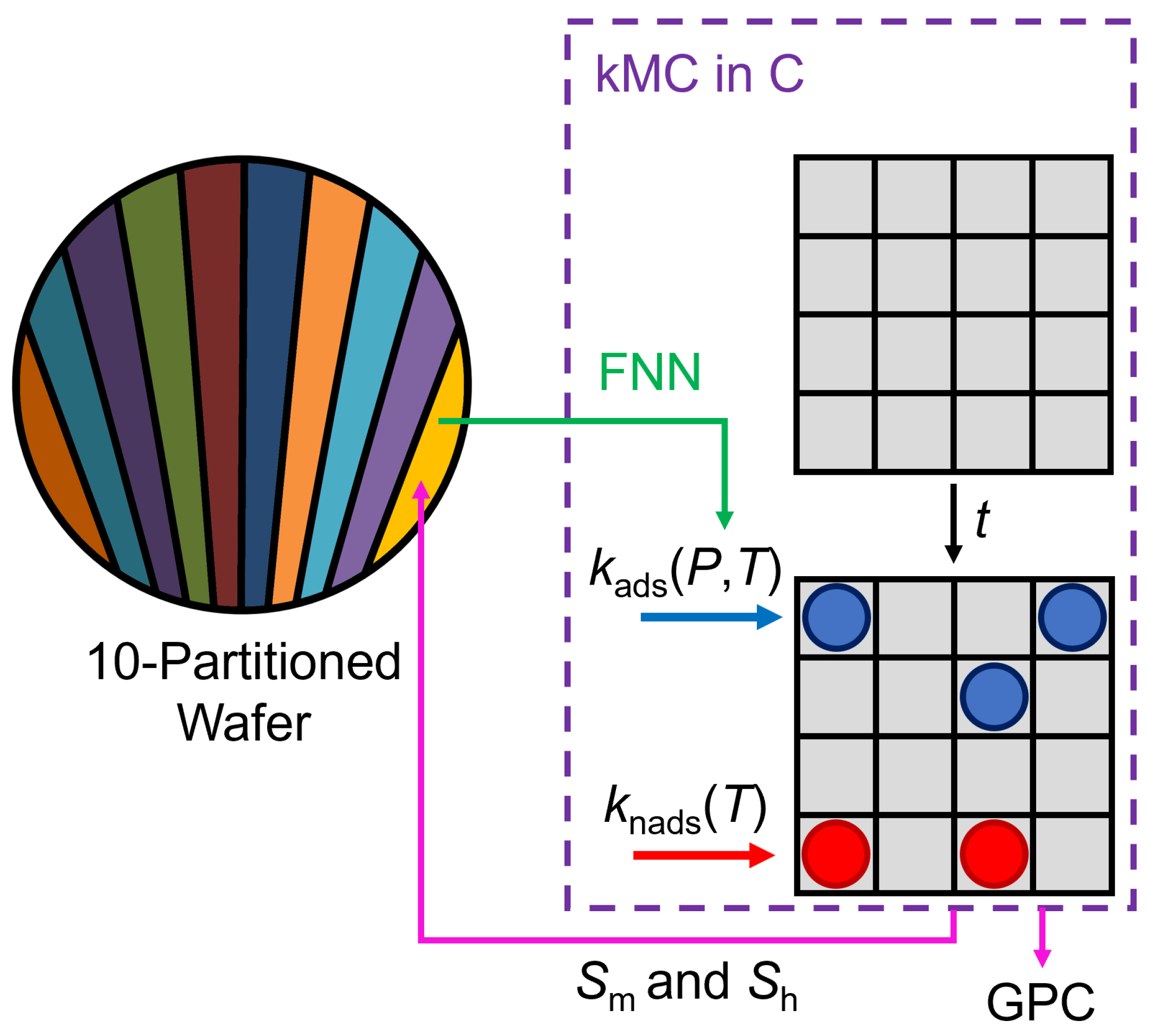
2.1. Atomistic Modeling

The development of an atomistic model is imperative for the calculation of reaction rate constants for rate-determining reactions involved in each step of the ABC, AS-ALD process. This work utilized an inhibitor, acetylacetone (Hacac), a precursor, bis(diethylamino)silane (BDEAS), and an oxidant, ozone (O₃) for a substrate composed of a non-growth area, aluminum oxide (Al₂O₃), and growth area, silicon oxide (SiO₂) where all reaction rate pathways are elucidated in several reference works [20,30]. The surface morphologies for Al₂O₃ and SiO₂ were assumed to be pure in the $\alpha$ [29] and $\beta$ [31] phases, respectively. Two types of reaction rate constants, the pressure and temperature-dependent adsorption, $k_{ads}(P,T)$, and temperature-dependent nonadsorption, $k_{nads}\left(T\right)$, are computed through Collision Theory and the Arrhenius equation, which depend on multiple variables including the sticking coefficient, $\sigma$, for adsorption reactions and the activation energy, $E_A$, and pre-exponential factor, $\nu$, (evaluated using Transition State Theory) for nonadsorption reactions. Equations for the pressure and temperature-dependent Collision Theory and the temperature-dependent Arrhenius model are described as follows:

$$k_{ads}=\frac{P{A}_{site}\sigma }{Z\sqrt{2\pi m{k}_{B}T}}$$

(1)

$$k_{nads}=\nu exp\left(-\frac{E_A}{RT}\right)$$

(2)

where P is the surface pressure of the reagent, $A_{site}$ is the surface area of the active site, Z is the coordination number, m is the atomic mass of the adsorbate species, $k_B$ is the Boltzmann constant, T is the ambient operating temperature of the reactor, and R is the ideal gas constant. Additionally, some thermophysical parameters of species such as the specific heat capacity, standard state enthalpy and entropy, density, dynamic viscosity, and thermal conductivity, are needed to reduce the degrees of freedom for the heat transfer dynamics in the macroscopic computational fluid dynamics (CFD) simulations. This work obtains sticking coefficient parameters for various species through an exhaustive literature search where the sticking coefficients for Hacac [13], BDEAS [32], and O₃ [33] were also determined by selecting sticking coefficients from species that are molecularly similar to the species in this work such as that of Hacac, which were validated with experimental processing times [30] to reach full coverage. Thermophysical property data were obtained from the National Institute of Standards and Technology (NIST) database and Material Safety Data Sheets (MSDS) from online references, experimental works, and databases through Ansys Chemkin. Thermophysical property data not found in literature references are calculated through first principles quantum mechanics computations using density functional theory (DFT), nudged elastic band (NEB) methods, and quasi-harmonic approximation (QHA) calculations through the open-source software, Quantum ESPRESSO. The reaction rate constant parameters and thermophysical property data are detailed by Yun et al. (2022a, 2023) [20,22].

2.2. Mesoscopic Modeling

The AS-ALD processing occurs when the surface of the substrate is exposed to a reagent along the wall-fluid boundary layer. To replicate the stochastic nature of the surface-scale kinetics, this work employs a modified kinetic Monte Carlo (kMC) method based on the algorithm proposed by Bortz, Kalos, and Lebowitz that is sometimes referred to as the n-fold way or BKL algorithm [34]. Whereas the classic BKL algorithm employs a Markov chain that advances the entire grid with each step, the modified kMC used in this project employs a Markov chain that only advances one site of the grid with each step. Specifically, the modified kMC randomly selects a site from the overall grid, followed by a random selection of a reaction pathway j, which then advances the internal timer of the kMC system with the following formulas:

$$k_{tot}=\sum _{i=1}^N{k}_i$$

(3a)

$$\sum _{i=1}^{j-1}{k}_i\le {\gamma }_1{k}_{tot}\le \sum _{i=1}^j{k}_i\mathrm{where}j=1,2,\dots ,N$$

(3b)

$$\delta t=-\frac{ln{\gamma }_2}{k_{tot}M}\mathrm{where}t\to t+\delta t$$

(3c)

where $k_{tot}$ is the sum of all possible reaction pathways for a single active site, ${\gamma }_1,{\gamma }_2\in (0,1]$ are uniformly chosen random numbers, $\delta t$ is the time evolution that is iteratively summed to the total process time t and represents the time for the active site to convert to the next state, and M is the number of total active sites. One advantageous modification to the conventional BKL approach is the inclusion of the number of available active sites (e.g., the number of active sites that have not reached a final state or are unoccupied) to the time evolution described by Equation (3c). With a decreasing number of available active sites, the probability of adsorption decreases to account for the fact that incoming reagents are less likely to encounter reactive substrate sites, thus causing the time evolution to increase. Additionally, M resembles the changing probability of unoccupied sites due to the nonspontaneous nature of the final reactions for Steps A, B, and C to form the terminated product. Since the number of unoccupied sites decreases with increasing process time, the probability of reagent adsorption will decrease, which builds on the assumptions made by Bortz et al. (1975) [34] and Gillespie (1976) [35]. For example, Kim et al. (2020) accounted for the role of unoccupied sites and steric hindrance effects in their Monte Carlo simulation through a random point searching methodology for an Al₂O₃/SiO₂ substrate [36]. Klement et al. (2021) also considered the role of adsorbate collisions and unoccupied active sites on the surface of the substrate for an AS-ALD process on a TiO₂/SiO₂ substrate [37]. This work similarly adopts the random site selection approach while including steric hindrance effects associated with the bulky properties of BDEAS and the free rotation of the adsorbed species, which has been addressed in prior work [20].

To optimize the simulation efficiency and compatibility with multiphysics software, Ansys Fluent, for computational fluid dynamics (CFD) simulations, the kMC script is conducted in the C programming language and utilized with various C compilers including GNU’s GCC and Intel oneAPI’s ICX, where CPU times are examined in Section 3. Additionally, C language has a stronger affinity for running parallel tasks compared to programming languages like Python, which further enhances the speed of the computation.

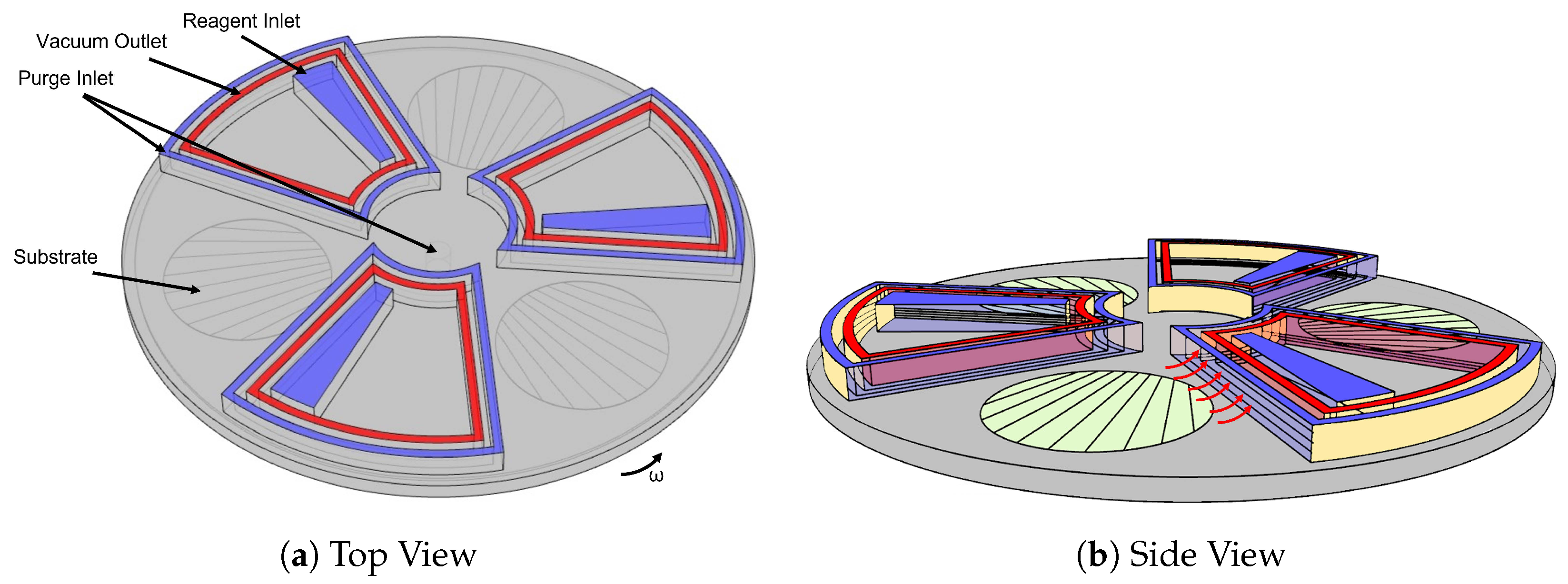
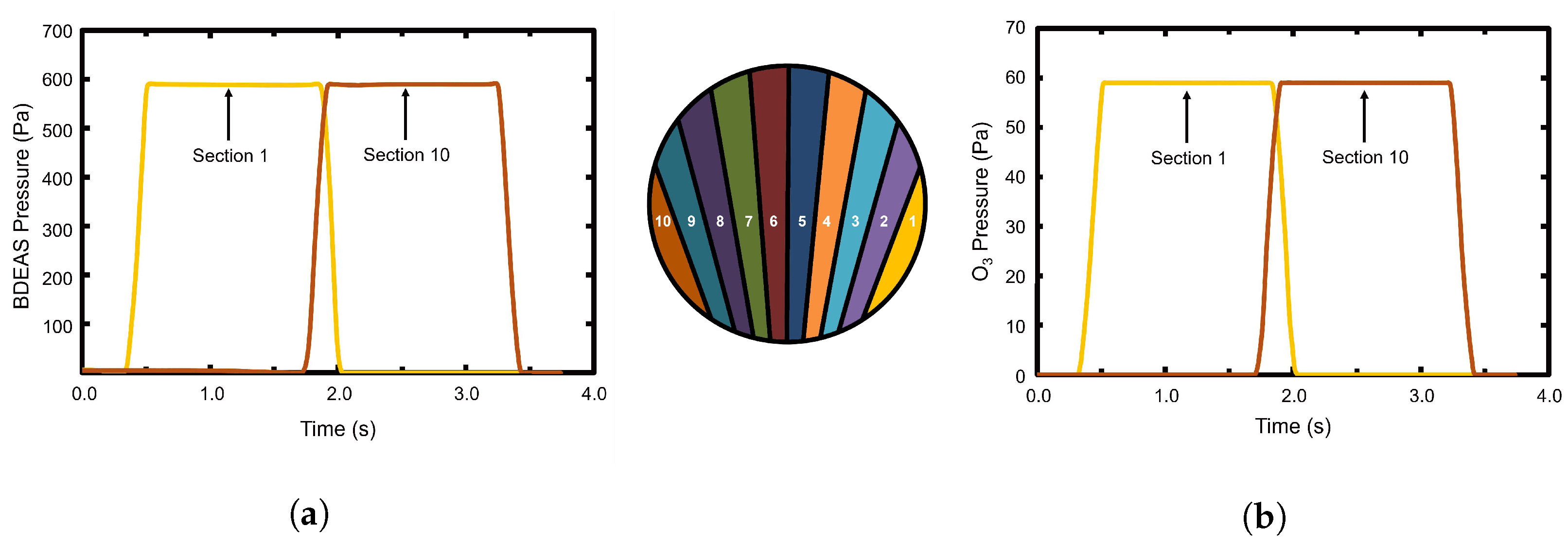
2.3. Macroscopic Modeling

The reaction rate constants used in the kMC simulation are dependent on the surface pressure and temperature, as well as whether the reactions are adsorption or nonadsorption reactions. The dynamics of the surface pressure and temperature depend on the design or geometry and the operating conditions of the reactor used to conduct the AS-ALD process. This work adopts a spatial, rotary reactor configuration that was previously developed [22] and illustrated in Figure 1. The three-dimensional (3D) reactor is optimized geometrically and the operating conditions are methodically chosen to reduce reagent intermixing while establishing uniform substrate exposure to reagent upon entry to the reaction zones. The reactor is operated under isothermal conditions; thus, the surface temperature profile is uniform and fixed spatiotemporally, and under isobaric conditions for total reactor pressure. Due to the small volume and sizing of the reactor with height in length scales of ${10}^{-3}$ m, a laminar model is specified for the fluid dynamics [38]. Additionally, constant inlet flow rates, reagent concentrations, outlet flow rates, and plate rotation speeds are defined with total inlet and outlet flow rates being equal, which are detailed in

Table 1. Operating conditions of the rotary reactor defined to the multiscale CFD simulation.

Operating Condition	Value
Reactor Pressure	1330 Pa
Reactor Temperature	523 K
BDEAS Mole Fraction	0.50
O3 Mole Fraction	0.05
Inlet Mass Flow Rate	2.00 × 10−5 kg/s

.

It is also illustrated that the substrate is partitioned into 10 sections to collect the spatiotemporal behavior of deposition rate and pressure field data. Each partitioned section is assigned an index for identification purposes that is depicted in Figure 2.

The rotary reactor is also discretized into a dynamic mesh comprising tetrahedral and triangular cells that are geometrically constructed through mesh quality criteria defined by the software, Ansys Fluent. A dynamic mesh is methodically defined to perform re-meshing steps that maintain the mesh quality through each movement of the mesh.

Computational fluid dynamics (CFD) is performed to study the characteristics of the reagent flow along the surface of the substrate by numerically and simultaneously solving the transport phenomena equations for mass, momentum, and heat, which are defined as follows:

$$\frac{\partial \rho }{\partial t}+\nabla ·\left(\rho \overrightarrow{v}\right)=S_m$$

(4)

$$\frac{\partial }{\partial t}\left(\rho \overrightarrow{v}\right)+\rho \left(\overrightarrow{v}·\nabla \right)\overrightarrow{v}=-\nabla P+\nabla ·(\stackrel{̿}{\tau })+\rho \overrightarrow{g}+\overrightarrow{F}$$

(5)

$$\frac{\partial }{\partial t}\left(\rho E\right)+\nabla \left(\overrightarrow{v}(\rho E+P)\right)=-\nabla (\sum h_j{\overrightarrow{J}}_j)+S_h$$

(6)

where $\rho$ represents the density of the reagent, $\overrightarrow{v}$ is the reagent velocity, $S_m$ is the reagent or byproduct consumption and generation source rate, respectively, P is the pressure of the gas-phase species, $\stackrel{̿}{\tau }$ is defined as the rank-two stress tensor, $\overrightarrow{g}$ is the gravitational constant, $\overrightarrow{F}$ is the body force subjected onto the gas-phase species, E is the internal energy of the system, $h_j$ is the sensible enthalpy of the species, j, $J_j$ is the mass diffusion flux rate of species, j, and $S_h$ is the heat transfer consumption or generation source rate. The CFD simulation employs a pressure-based coupled solver with a first-order, transient, and implicit numerical solver method with a fixed timestep size of 0.001 s.

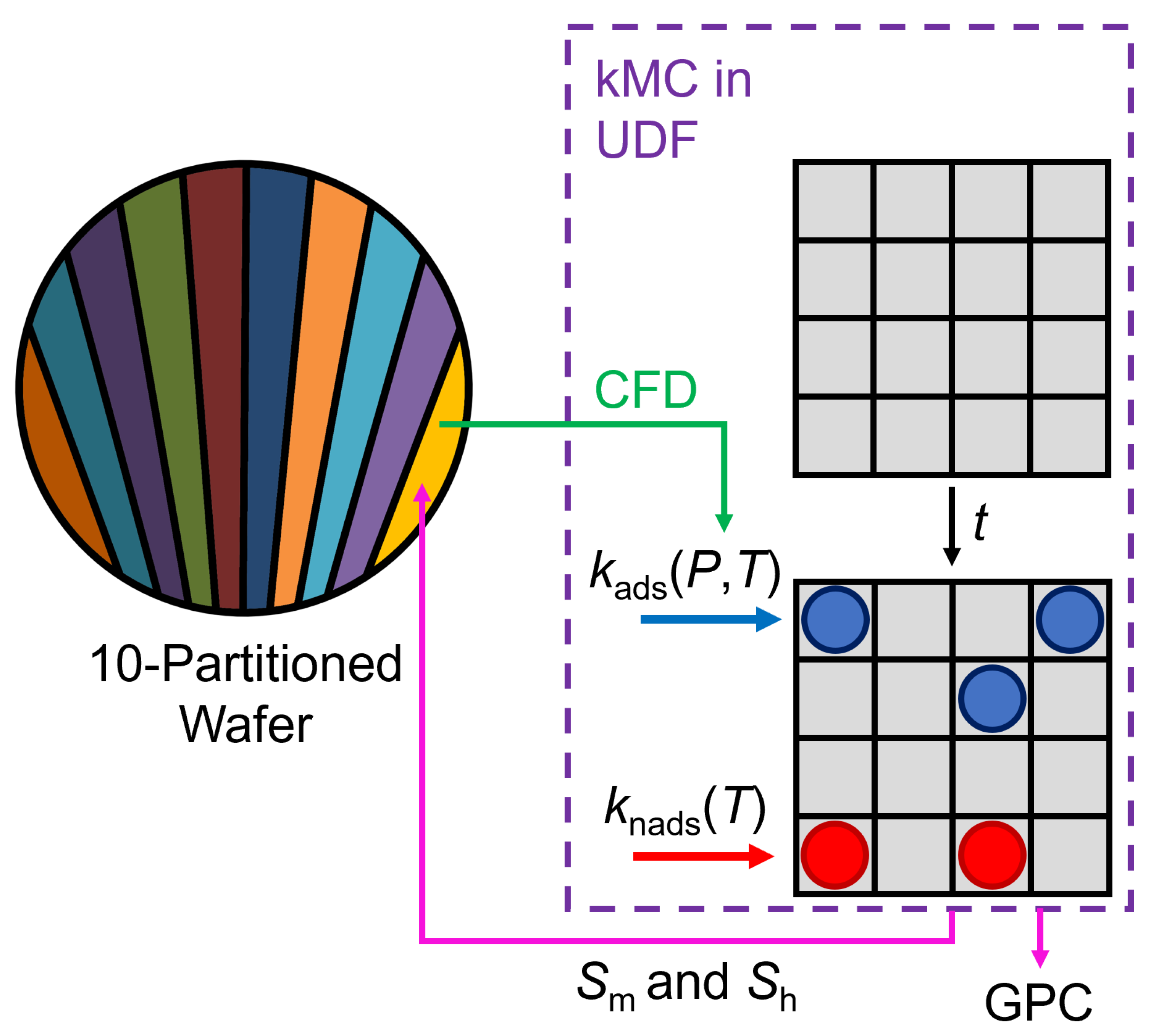
2.4. Multiscale Modeling

The conjunction of the atomistic, mesoscopic, and macroscopic simulations produces a multiscale model that enables various time and length scales to be examined. The multiscale model, depicted in Figure 2, is constructed through the application of a user-defined function (UDF) script that is written in the C programming language and integrates C-based macros that are inherent to the Ansys Fluent program. UDFs allow users to customize tasks for specific computations that are not available in the software client. To discuss the spatiotemporal aspects of the simulation, the program partitions the substrate into 10 sections in the radial direction of the center of mass of the rotary reactor, which is illustrated in Figure 1. The multiscale simulation begins by performing CFD for a timestep size of 0.001 s to calculate the pressure field data on the substrate surface, which is partitioned into 10 sections. This reagent pressure data are calculated through an area-averaged approach for each section on the wafer and is then sent to UDF to calculate reaction rate constants for adsorption and nonadsorption reactions. Next, the kMC script is executed for each wafer section in a parallel computation procedure until the processing time, t, reaches the timestep size of 0.001 s where the output, growth per cycle (GPC), and the source generation and consumption rates for mass and heat are calculated. It is notable that since the reactor is operating under isothermal conditions, heat generation and consumption rates are negligible for this work. Next, the source generation and consumption mass source rate is defined to the surface boundary condition for each section of the wafer, where the next iteration for the multiscale simulation is executed repetitively until the wafer exits the reaction zone. To ensure computational efficiency is sufficient, this work adopted various CPU (Central Processing Unit) nodes comprising 36 and 48 cores with 384 GB and 512 GB of RAM (Random Access Memory), respectively.

A consequence of the partitioning is that earlier sections of the wafer partition will enter the reaction zone before later sections of the wafer where a noticeable delay in complete saturation exposure would be observed. This consideration is depicted from the multiscale simulation results in Figure 3, which illustrates the spatiotemporal behavior of the area-averaged surface pressure for BDEAS and O₃ for a constant rotation speed of 0.56 rad/s.

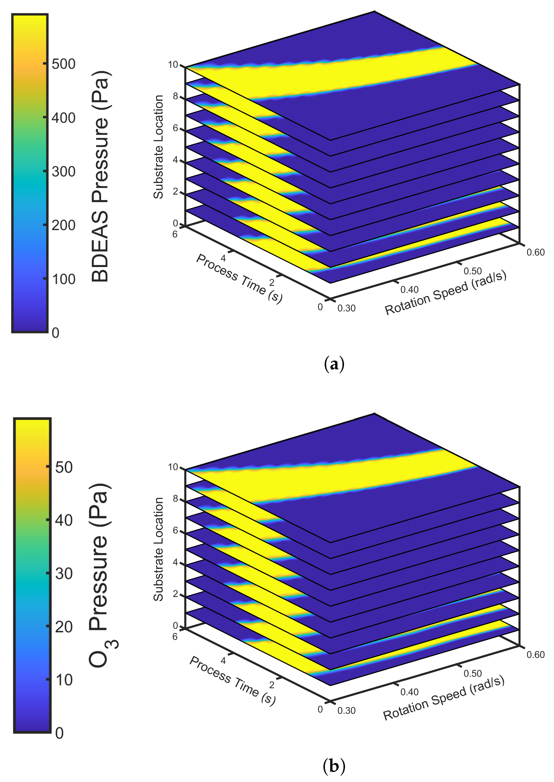
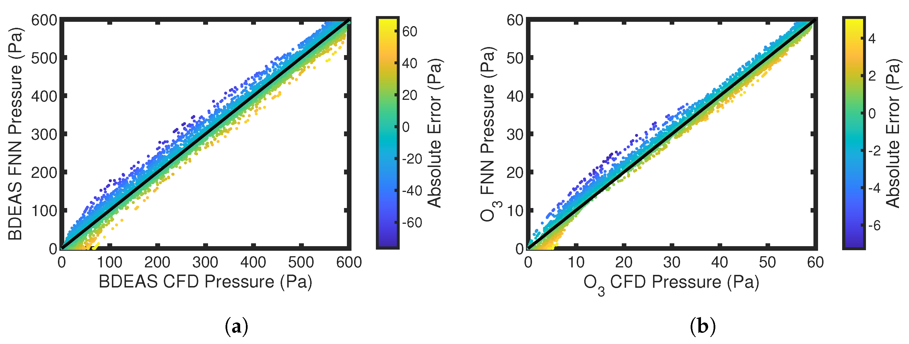
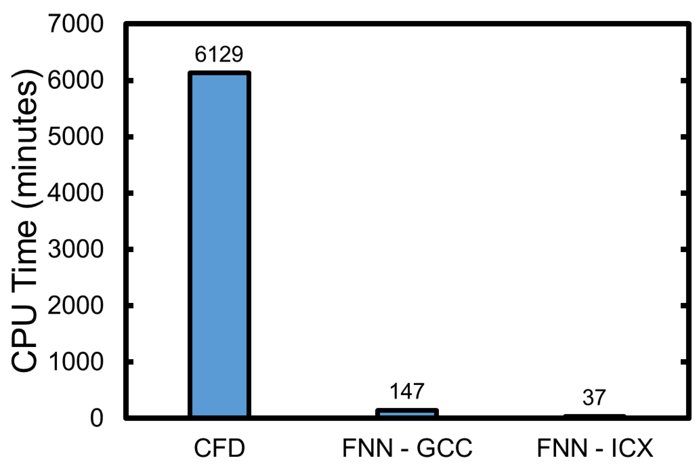
3. Pressure Field Generation through Machine Learning

One disadvantage of multiscale simulations is the computational complexity and inefficiency when data must be gathered in short time intervals. The multiscale model defined in Section 2 and shown in Figure 2 may require minimum simulation times of 3 days and maximum simulation times of 14 days, depending on the rotation speed of the wafer that is defined to the multiscale model. Lower rotation speeds increase the residence time of the wafer in the reaction zones, which increases the computation time. Thus, this work proposes a machine learning approach to correlate a multi-input-single-output (MISO) data set, to produce pressure field data in place of pressure field data generated through CFD.

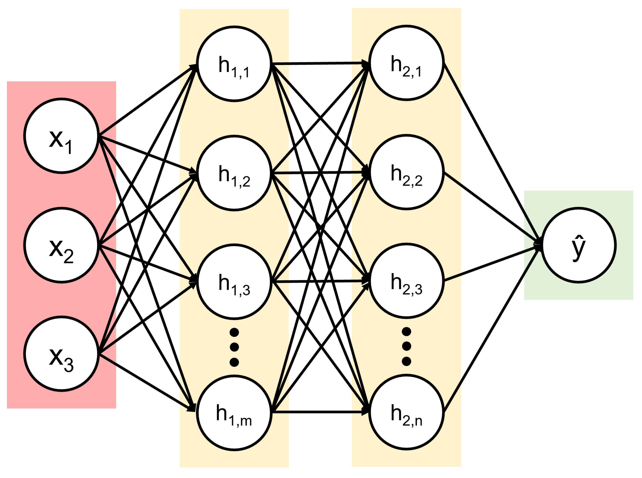
Feedforward Neural Network for MISO System

A feedforward neural network (FNN) model is generated for a multi-input system composed of three variables (rotation speed, process time, and substrate location) to calculate a single predicted output, the growth per cycle (GPC). This FNN model is illustrated in Figure 4, which describes the nodal connections that are conducted to train the FNN.

The FNN was constructed using two hidden layers, each including 30 neurons to train and test data sets of 240,000 and 120,000 data points for BDEAS and O₃ pressure, respectively. It is notable that the Hacac pressure is not included in this work, since the GPC is a measurement taken from the growth area of the substrate. A two-hidden layer FNN is described by the following equations that describe the training of the FNN:

$$\begin{array}{cc}\hfill \widehat{y}& =W_2{H}_2+B_2\hfill \\ \hfill H_2& =f(W_1{H}_1+B_1)\hfill \\ \hfill H_1& =f(W_{0}X+B_0)\hfill \end{array}$$

where $\widehat{y}$ is the predicted output, GPC, $X\in {\mathbb{R}}^m$ is the input vector comprising $m=3$ input parameters (rotation speed, process time, and substrate location), $W_0\in {\mathbb{R}}^{n\times m},W_1\in {\mathbb{R}}^{n\times n},W_2\in {\mathbb{R}}^n$ are weights where $n=30$ neurons for each hidden layer, $B_0\in {\mathbb{R}}^n,B_1\in {\mathbb{R}}^n,B_2\in \mathbb{R}$, and $f(·)$ is the rectified linear unit (ReLU) activation function. Additionally, the FNN models for BDEAS and O₃ were generated by using a training size of 90% and testing size of 10% using the Adam optimizer, a learning rate of 0.004, and by minimizing the mean squared error (MSE), which was conducted through the open-source Python library, TensorFlow.

Predicted BDEAS and O₃ pressure data from the FNN model are depicted in Figure 5 with the BDEAS and O₃ FNN models having MSEs of 0.0143 and 0.0121, respectively. Figure 3 illustrates that substrate location affects the processing time required for the substrate to become completely exposed to the reagent due to the time delays for the sections to enter the reaction zone. Furthermore, increasing rotation speed also increases the time needed for the substrate to observe full exposure to the reagent, which is reflective of the operation of the rotary reactor while the residence time of the wafer in the reaction zone increases with decreasing rotation speed. The precision and accuracy of the FNN model are presented in Figure 6, which plots a sample of all data points to illustrate the absolute error of the FNN predicted pressures to the multiscale CFD pressures for BDEAS and O₃. Results demonstrate that a majority of points have a marginal error, thus enabling the substitution of the FNN model in place of the pressure data generated from the multiscale CFD simulation.

Additionally, with the integration of the FNN model, the multiscale model outlined in Figure 2 substitutes FNN in place of CFD while retaining the conjunction to the kMC script, which is still presented in the C language while removing user-defined function macros from Ansys Fluent’s programming language in Figure 7. From the modified multiscale model, simulation time is dramatically reduced from timescales of days to minutes by employing TensorFlow and the Intel oneAPI ICX C compiler toolkit, which is conveyed in Figure 8. The efficiency of the modified multiscale model with FNN integration is sufficient to progress to control work, which requires abundant data generation to produce an accurate input-output model that is described in Section 4.

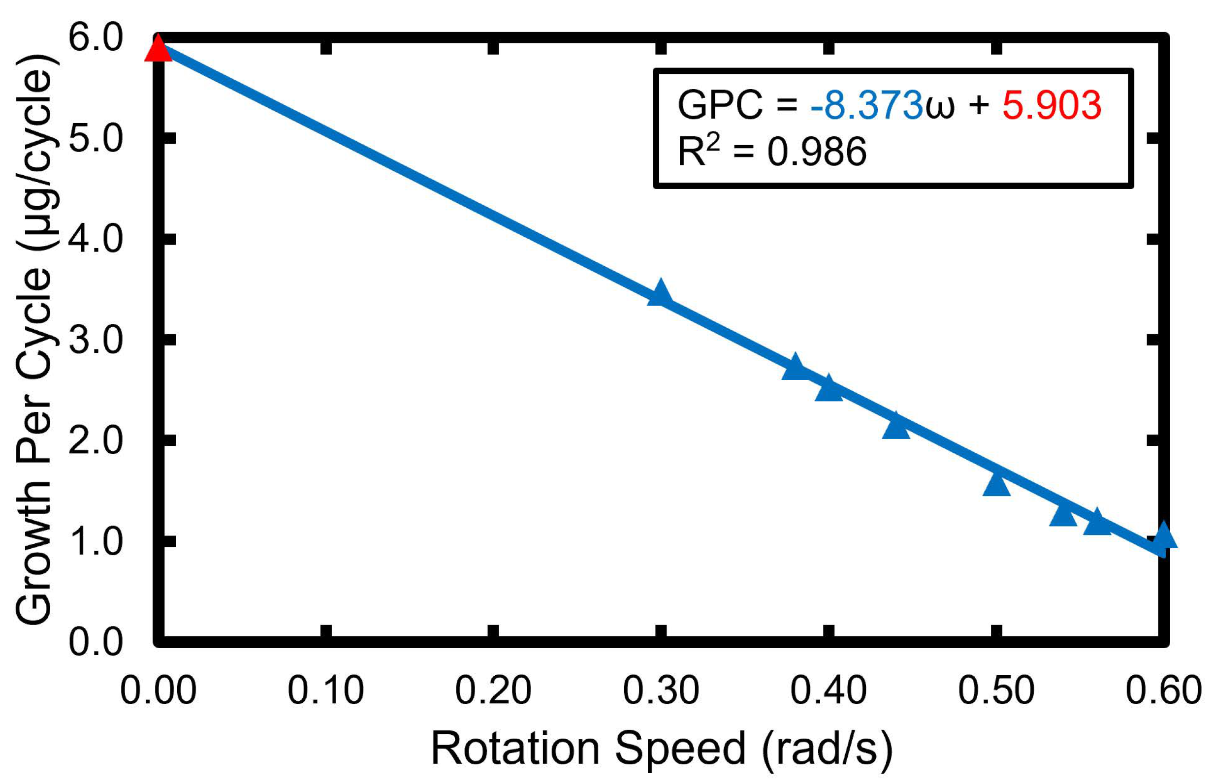
4. R2R Modeling of the SISO Process

To develop a paradigm for the control of AS-ALD, the general procedures conducted in in vitro environments are first examined to provide insight into the controller mechanism. Area-selective atomic layer deposition (AS-ALD) is a cyclical process composed of a three-step, ABC, procedure composed of inhibition, chemical adsorption, and oxidation sub-cycles that occur in short intervals. Due to these short intervals, which occur in the range of 1 to 5 s [29,39], in situ monitoring cannot be performed due to time delays associated with the controller. Thus, ex-situ statistical process control (SPC) methods such as run-to-run (R2R) control have been employed in the semiconductor manufacturing industry to regulate operating conditions by employing offline adjustments to the input parameter(s) [23] after completion of a batch run or in this work, a cycle of AS-ALD, to return the process to the setpoint. This work will study the impact of these disturbances on the growth per cycle (GPC) on the growth area of the substrate. Thus, Step A of the ABC AS-ALD process is not considered for this component of the R2R control framework.

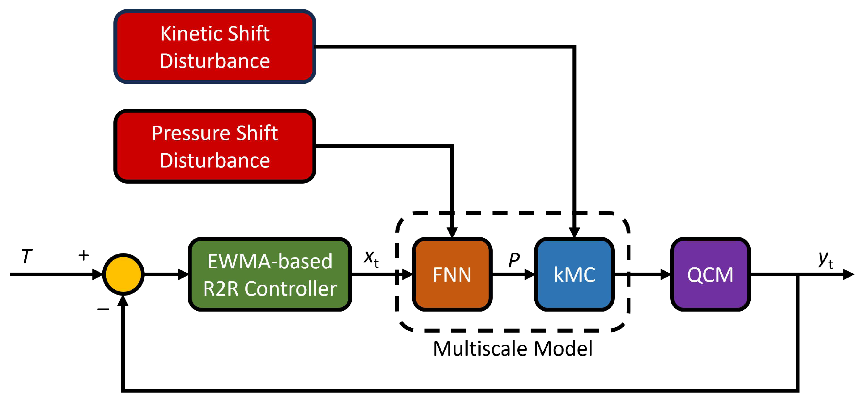
4.1. Run-to-Run Controller Framework

The R2R controller action is conducted by receiving measured output data that are produced from the multiscale model and portrayed in Figure 9. The multiscale simulation provides the substrate rotation speed as an input variable to evaluate surface pressure data for BDEAS and O₃. Additionally, constant shift disturbances are applied to the FNN or kMC components of the multiscale model in the form of a multiplicative factor to deviate the output, growth per cycle (GPC), from the setpoint. In industrial applications, a Quartz Crystal Microbalance (QCM) [40] is used to measure the GPC by taking the reactor system offline. The resulting GPC is then sent to the R2R controller where an exponentially weighted moving average method is performed to calculate an updated rotation speed for the subsequent batch run, where the formulation is discussed in greater detail in Section 4.2.

4.2. Exponentially Weighted Moving Average Approach to Run-to-Run Control

Each R2R controller uses a statistical algorithm such as the exponentially weighted moving average (EWMA), the double exponentially weighted moving average (dEWMA), and the autoregressive moving averages (ARMA), to perform controller correction based on the error of the measured output parameter from the target or setpoint. This work will employ the EWMA method to implement controller action due to its capability of detecting and mitigating small-magnitude shift disturbances [41].

The EWMA method relies on a linear regression model of multiscale data of the output variable, growth per cycle (GPC) on the growth area of the substrate, for a range of the input variable, substrate rotation speed, which are obtained offline [42]. The linear regression model is defined as follows:

$$\widehat{y}=\alpha +\beta u$$

(7)

where $\widehat{y}$ is the estimated deposition rate evaluated by the linear regression model, $\alpha$ is the bias or intercept, $\beta$ is the process gain or slope, and u is the input variable. The linear model produced from open-loop data produced from the multiscale simulation of the output, GPC, and input, rotation speed, is presented in Figure 10. The controller-adjusted input variable, ${\mu }_t$ will then be calculated based on the deviation of the output variable from the setpoint, T.

$${\mu }_t=\frac{T-a_t}{b}$$

(8)

where $b=\beta$ and $a_t$ is the adjusted bias at batch run t where $\alpha =a_0$, which is evaluated through an exponentially weighted moving average. A predicted intercept is evaluated by recursively summing the errors from each batch run [23], and is defined by the following expression:

$$a_t=\lambda (y_t-b{u}_{t-1})+(1-\lambda )a_{t-1}$$

(9)

where $y_t$ is the measured GPC evaluated from the multiscale modeling simulation and $\lambda \in (0,1]$ is a self-determined weighting parameter that is used to preferentially balance the impact of older data on newer data [43]. $\lambda$ also has a significant role in controlling oscillatory behavior, which is analogous to the role that integral action conducts in proportional-integral (PI) controllers. Thus, lower $\lambda$ is suggested for the detection of small-magnitude shift disturbances, as recommended by Montgomery (2013) [44] and Lucas and Saccucci (1990) [45]. An important characteristic of performing an EWMA weight of the intercept of the linear model is the ability to tune modeling data to implement controller action by assuming a constant slope [42]. Such methodology is established by the assumption that disturbances will generally affect all elements of the data-fitted model, thereby translating all points in the model in the form of a tuning strategy. The adoption of this methodology enables all model-fitted open-loop data to impact the controller update to the input parameters without requiring the generation of a new model for each observation of a disturbance, which may require an abundance of data generation.

4.3. Limitations of the EWMA-Based R2R Controller

Arguably, the EWMA approach has some limitations that are notable for this work. For instance, the EWMA method will utilize a constant $\lambda$, which must be determined through extensive experimental studies and is dependent on the magnitude of the shift disturbances [44]. For example, if a large-magnitude error is produced from a shift disturbance with a low $\lambda$, additional batch runs would be required for the controller to implement sufficient controller action to minimize the offset. In realistic settings, the magnitude of the shift disturbance is unpredictable, which is why this work focuses on the integration of a constant and minor shift disturbance only. This particular EWMA method also neglects the potential for noise and drift disturbances, which are frequent issues often encountered in industrial applications for semiconductor processing and are attributed to sudden changes in the operation of the reactor [46]. Additionally, this EWMA approach assumes that complete feedback control is implemented for each batch run, thus the reactor will be required to be taken offline after each batch run to measure the output parameter using a Quartz Crystal Microbalance to measure the GPC. This procedure may be impractical for realistic control and is inefficient for achieving high-throughput semiconductor generation, but serves as a starting point towards controller models that implement controller action using an open-loop approach, such as the previously proposed self-tuning model [46]. It is notable that self-tuning strategies using ARMA models are beneficial for mitigating disturbances for drift and noise, but are ineffective for bringing process stability toward the setpoint but rather maintain the process within standard deviations from the setpoint [47].

4.4. Compensation of Shift Disturbances

This work considers the effects of two shift disturbances that are intended to deviate the reactor operation from idealistic conditions. One of these shift disturbances includes a pressure shift disturbance that negatively or positively impacts the GPC of the system by including a constant shift variable intended to decrease or increase the magnitude of the pressure field data in the FNN model. Recall that the GPC is a parameter that is evaluated from the surface coverage computation from the kMC simulation. The reaction rate constants for nonadsorption and adsorption reactions are computed from the temperature-dependent Arrhenius model and the temperature- and pressure-dependent Collision Theory model, respectively. The integration of pressure and kinetic shift disturbance is intended to increase or decrease the magnitude of the reaction rate constants for the adsorption and nonadsorption reactions, thereby increasing or decreasing the computed surface coverage. For the pressure disturbance, a coefficient is introduced to the machine learning model to increase or decrease the pressure field data while for the kinetic disturbance, a coefficient is introduced to the computation of the total reaction rate constant, $k_{tot}$, which affects the time advanced computation in Equation (3c). It is notable that the kinetic shift disturbance is intended to perturb all reaction rate constants (adsorption and nonadsorption), by introducing a constant shift variable intended to decrease or increase their magnitude. The introduction of the pressure shift disturbance reflects the changes in the operating conditions such as that in the input, and kinetic disturbances resemble potential shift disturbances that may be unaccounted for during the AS-ALD process such as equipment failure.

5. Closed-Loop Simulation Results

The objective of the R2R controller is to manipulate the rotation speed of the wafer, which congruently affects the residence time of the substrate within the reaction zone. The residence time is a direct indicator of how much reagent is deposited onto the surface of the substrate, where GPC increases with increasing residence time. By subjecting the AS-ALD process to pressure and kinetic shift disturbances in the multiscale model, the R2R controller must minimize the error from the setpoint by adjusting the rotation speed. This section will examine the response of the R2R controller to various disturbances that positively and negatively affect the GPC on the substrate.

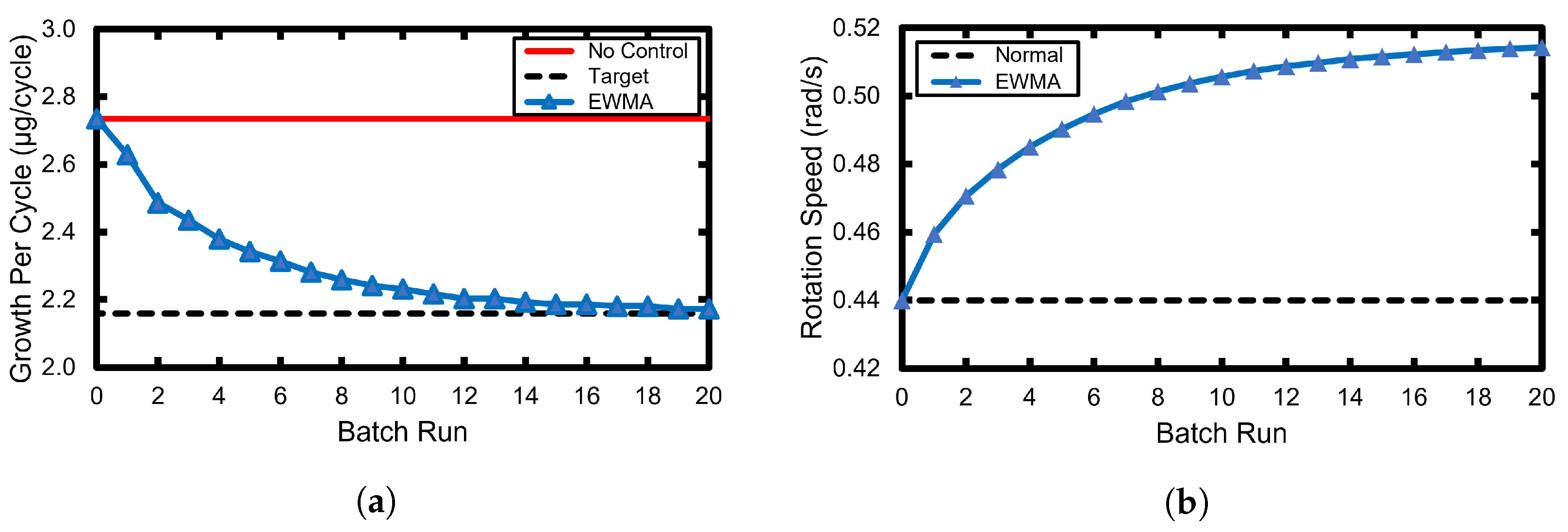
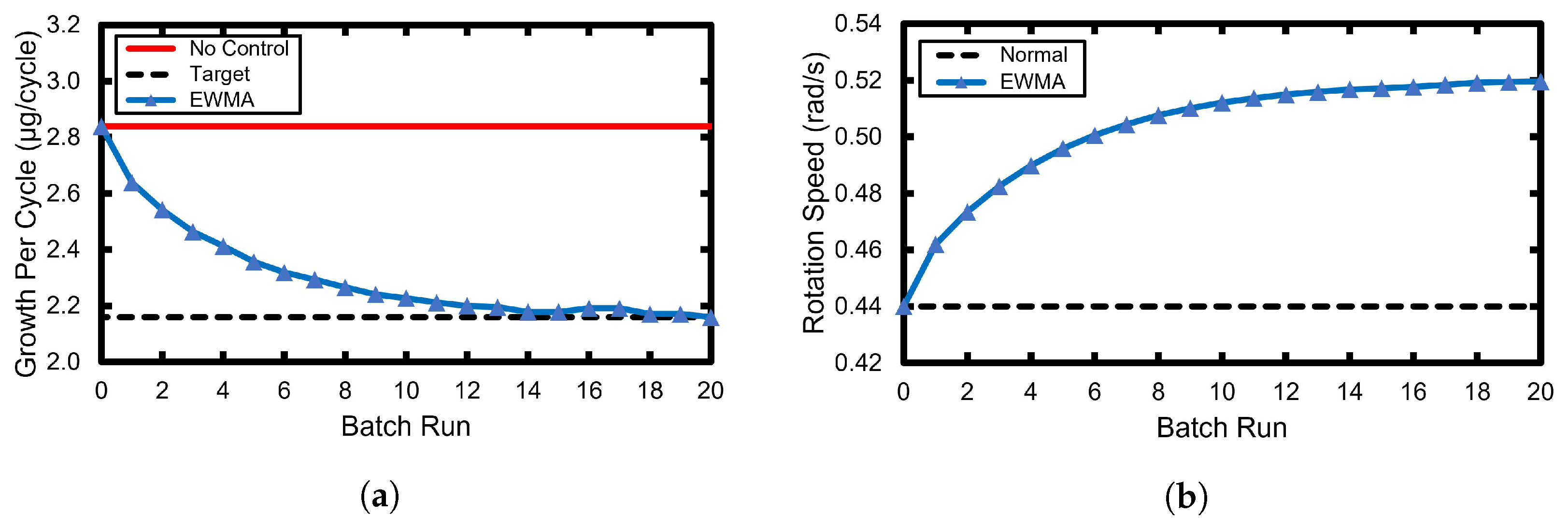
5.1. Closed-Loop Response to Pressure Disturbances

Pressure disturbances are oftentimes encountered in semiconductor fabrication due to potential changes in the fluid dynamics that are attributed to byproduct generation or changes to the inlet conditions. The pressure has a profound impact on the ability for adsorbates like BDEAS and O₃ to interact with the substrate surface via Collision Theory. Positive shift disturbances on the BDEAS and O₃ pressures were introduced to the FNN model for factors of 0.2 and 0.1, respectively, and their response is illustrated in Figure 11 using an EWMA weight of $\lambda =0.2$. Findings illustrate that the EWMA approach successfully overcomes the effects of the disturbance within 19 batch runs in Figure 11a by increasing the rotation speed of the wafer depicted in Figure 11b in order to reduce the residence of the wafer in the reaction zone. The results decrease the GPC to the desired setpoint. However, the result suggests that a substantial initial response is needed for the controller to mitigate the effects of the disturbance by requiring lesser batch runs to reach the setpoint. In addition to positive shift disturbances on the BDEAS and O₃ pressures, negative shift disturbances were introduced to the FNN model for pressure generation using factors of 0.2 and 0.1, respectively. The results of the R2R controller action are presented in Figure 12 using an EWMA weight of $\lambda =0.2$. It is observed that the R2R controller detects the minor shift disturbances induced to the GPC by decreasing the rotation speed in Figure 12b thereby increasing the residence time of the wafer in the reaction zone. The result is depicted by a steady increase in the GPC in Figure 13a where the setpoint is reached at 14 batch runs.

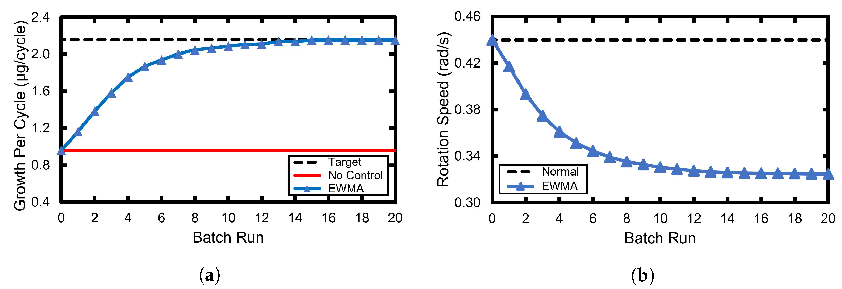
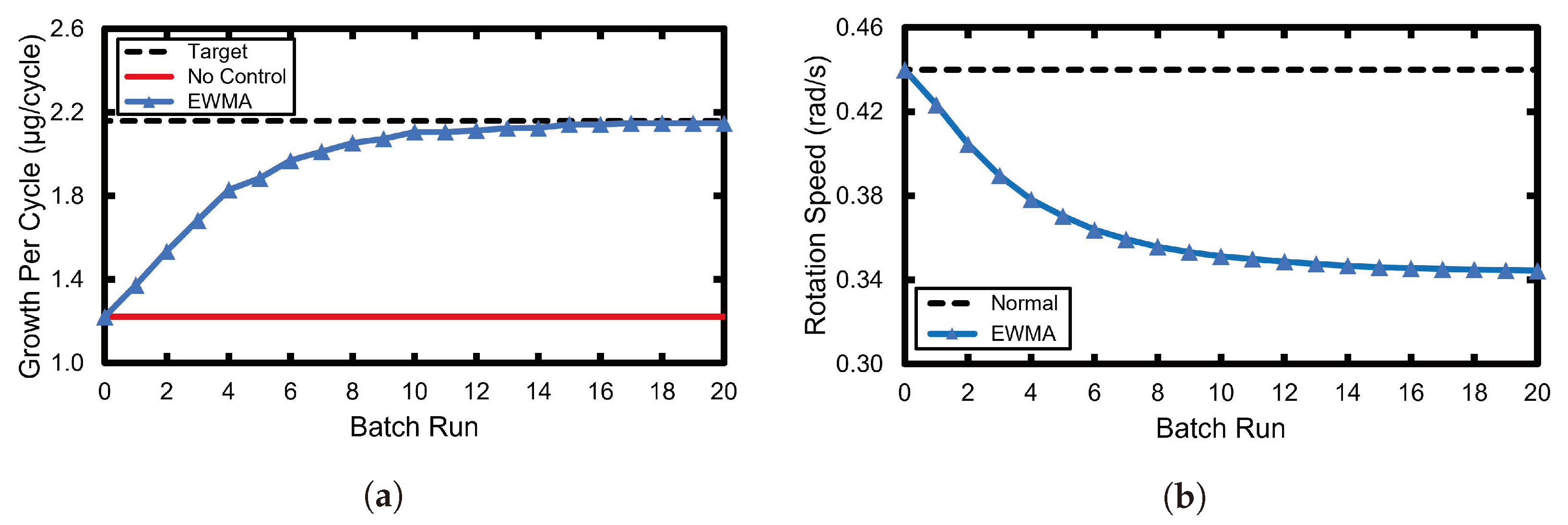
5.2. Closed-Loop Response to Kinetic Disturbances

Kinetic disturbance factors were applied to the kMC simulations for Steps B and C of the AS-ALD process to represent the perturbation of unknown disturbances that are applied to all reactions (adsorption and nonadsorption). Figure 13 illustrates the R2R controller response when subjecting the kMC simulations for Steps B and C to a constant kinetic disturbance factor that increases the GPC from the desired setpoint. The R2R controller uses an EWMA weight of $\lambda =0.2$, which indicates that the setpoint is reached at 14 batch runs in Figure 13a by increasing the rotation speed presented in Figure 13b to compensate for the excess deposition onto the growth area of the substrate. In addition to subjecting the reaction rate constants to positive shift disturbances, negative shift disturbances were also applied separately to Steps B and C kMC simulations, with results pictured in Figure 14. An R2R controller with an EWMA weight of $\lambda =0.2$ increased the residence time of the substrate in the reaction zone by decreasing the rotation speed of the wafer depicted in Figure 14b. The result of the adjustment increases the GPC to the setpoint after 16 batch runs, which is shown in Figure 14a.

6. Conclusions

This work developed a run-to-run controller with an exponentially weighted moving average approach to overcome the effects of various pressure and kinetic shift disturbances for an area-selective atomic layer deposition rotary reactor, which are often observed in industrial applications for semiconductor manufacturing. To facilitate the process of generating data, this work developed an in silico multiscale model that integrates machine learning through a feedforward neural network to generate surface pressure data that are conjoined to a kinetic Monte Carlo simulation written in the C programming language that evaluates the growth per cycle on the growth areas of a semiconductor substrate. An advantageous product of machine learning and C programming language integration for multiscale modeling is the substantial reduction in computation time from timescales of days to minutes. The run-to-run controller implemented input adjustment to the rotation speed of the rotary reactor to regulate the residence time of the substrate within the reaction zones, thereby allowing the controller to bring the process back to the setpoint within a minimum of 14 batch runs.

References

1. Bhalla, A. Silicon carbide semiconductors with wide bandgap for electric vehicles. ATZelectronics Worldw. 2021, 16, 18–21. [Google Scholar]
2. Anitha, V.C.; Banerjee, A.N.; Joo, S.W. Recent developments in TiO2 as n- and p-type transparent semiconductors: Synthesis, modification, properties, and energy-related applications. J. Mater. Sci. 2015, 50, 7495–7536. [Google Scholar] [CrossRef]
3. Petti, L.; Münzenrieder, N.; Vogt, C.; Faber, H.; Büthe, L.; Cantarella, G.; Bottacchi, F.; Anthopoulos, T.D.; Tröster, G. Metal oxide semiconductor thin-film transistors for flexible electronics. Appl. Phys. Rev. 2016, 3, 021303. [Google Scholar] [CrossRef]
4. Khakifirooz, M.; Fathi, M.; Wu, K. Development of smart semiconductor manufacturing: Operations research and data science perspectives. IEEE Access 2019, 7, 108419–108430. [Google Scholar] [CrossRef]
5. Zhang, A.; Lieber, C.M. Nano-bioelectronics. Chem. Rev. 2016, 116, 215–257. [Google Scholar] [CrossRef] [PubMed]
6. Chhowalla, M.; Jena, D.; Zhang, H. Two-dimensional semiconductors for transistors. Nat. Rev. Mater. 2016, 1, 16052. [Google Scholar] [CrossRef]
7. Khanna, V.K. Integrated Nanoelectronics: Nanoscale CMOS, Post-CMOS and Allied Nanotechnologies; Springer: New Delhi, India, 2016. [Google Scholar]
8. Loubet, N.; Hook, T.; Montanini, P.; Yeung, C.W.; Kanakasabapathy, S.; Guillom, M.; Yamashita, T.; Zhang, J.; Miao, X.; Wang, J.; et al. Stacked nanosheet gate-all-around transistor to enable scaling beyond FinFET. In Proceedings of the 2017 Symposium on VLSI Technology, Kyoto, Japan, 5–8 June 2017; pp. T230–T231. [Google Scholar]
9. Frieske, B.; Stieler, S. The “semiconductor crisis” as a result of the COVID-19 pandemic and impacts on the automotive industry and its supply chains. World Electr. Veh. J. 2022, 13, 189. [Google Scholar] [CrossRef]
10. Mohammad, W.; Elomri, A.; Kerbache, L. The global semiconductor chip shortage: Causes, implications, and potential remedies. IFAC-Pap. 2022, 55, 476–483. [Google Scholar] [CrossRef]
11. Shattuck, T.J. Stuck in the middle: Taiwan’s semiconductor industry, the U.S.-China tech fight, and cross-strait stability. Orbis 2021, 65, 101–117. [Google Scholar] [CrossRef]
12. Voas, J.; Kshetri, N.; DeFranco, J.F. Scarcity and global insecurity: The semiconductor shortage. IT Prof. 2021, 23, 78–82. [Google Scholar] [CrossRef]
13. George, S.M. Atomic layer deposition: An overview. Chem. Rev. 2010, 110, 111–131. [Google Scholar] [CrossRef] [PubMed]
14. Johnson, R.W.; Hultqvist, A.; Bent, S.F. A brief review of atomic layer deposition: From fundamentals to applications. Mater. Today 2014, 17, 236–246. [Google Scholar] [CrossRef]
15. Carver, C.T.; Plombon, J.J.; Romero, P.E.; Suri, S.; Tronic, T.A.; Turkot, R.B. Atomic layer etching: An industry perspective. ECS J. Solid State Sci. Technol. 2015, 4, N5005. [Google Scholar] [CrossRef]
16. Kanarik, K.J.; Lill, T.; Hudson, E.A.; Sriraman, S.; Tan, S.; Marks, J.; Vahedi, V.; Gottscho, R.A. Overview of atomic layer etching in the semiconductor industry. J. Vac. Sci. Technol. A 2015, 33, 020802. [Google Scholar] [CrossRef]
17. Chen, R.; Kim, H.; McIntyre, P.C.; Porter, D.W.; Bent, S.F. Achieving area-selective atomic layer deposition on patterned substrates by selective surface modification. Appl. Phys. Lett. 2005, 86, 191910. [Google Scholar] [CrossRef]
18. Chen, R.; Bent, S.F. Chemistry for positive pattern transfer using area-selective atomic layer deposition. Adv. Mater. 2006, 18, 1086–1090. [Google Scholar] [CrossRef]
19. Mackus, A.J.M.; Merkx, M.J.M.; Kessels, W.M.M. From the bottom-up: Toward area-selective atomic layer deposition with high selectivity. Chem. Mater. 2019, 31, 2–12. [Google Scholar] [CrossRef]
20. Yun, S.; Ou, F.; Wang, H.; Tom, M.; Orkoulas, G.; Christofides, P.D. Atomistic-mesoscopic modeling of area-selective thermal atomic layer deposition. Chem. Eng. Res. Des. 2022, 188, 271–286. [Google Scholar] [CrossRef]
21. Tom, M.; Yun, S.; Wang, H.; Ou, F.; Orkoulas, G.; Christofides, P.D. Multiscale modeling of spatial area-selective thermal atomic layer deposition. In 33rd European Symposium on Computer Aided Process Engineering; Kokossis, A.C., Georgiadis, M.C., Pistikopoulos, E., Eds.; Elsevier: Athens, Greece, 2023; Volume 52, Computer Aided Chemical Engineering; pp. 71–76. [Google Scholar]
22. Yun, S.; Wang, H.; Tom, M.; Ou, F.; Orkoulas, G.; Christofides, P.D. Multiscale CFD modeling of area-selective atomic layer deposition: Application to reactor design and operating condition calculation. Coatings 2023, 13, 558. [Google Scholar] [CrossRef]
23. Moyne, J.; Del Castillo, E.; Hurwitz, A.M. Run-to-Run Control in Semiconductor Manufacturing; CRC Press: Boca Raton, FL, USA, 2018. [Google Scholar]
24. Andrews, M. Critical Manufacturing redefines semiconductor MES. Silicon Semicond. 2022, 43, 38–41. [Google Scholar]
25. Tom, M.; Yun, S.; Wang, H.; Ou, F.; Orkoulas, G.; Christofides, P.D. Machine learning-based run-to-run control of a spatial thermal atomic layer etching reactor. Comput. Chem. Eng. 2022, 168, 108044. [Google Scholar] [CrossRef]
26. Yun, S.; Tom, M.; Ou, F.; Orkoulas, G.; Christofides, P.D. Multivariable run-to-run control of thermal atomic layer etching of aluminum oxide thin films. Chem. Eng. Res. Des. 2022, 182, 1–12. [Google Scholar] [CrossRef]
27. Yun, S.; Ding, Y.; Zhang, Y.; Christofides, P.D. Integration of feedback control and run-to-run control for plasma enhanced atomic layer deposition of hafnium oxide thin films. Comput. Chem. Eng. 2021, 148, 107267. [Google Scholar] [CrossRef]
28. Zhang, Y.; Ding, Y.; Christofides, P.D. Integrating feedback control and run-to-run control in multi-wafer thermal atomic layer deposition of thin films. Processes 2019, 8, 18. [Google Scholar] [CrossRef]
29. Mameli, A.; Merkx, M.J.M.; Karasulu, B.; Roozeboom, F.; Kessels, W.E.M.M.; Mackus, A.J.M. Area-selective atomic layer deposition of SiO2 using acetylacetone as a chemoselective inhibitor in an ABC-type cycle. ACS Nano 2017, 11, 9303–9311. [Google Scholar] [CrossRef] [PubMed]
30. Merkx, M.J.M.; Sandoval, T.E.; Hausmann, D.M.; Kessels, W.M.M.; Mackus, A.J.M. Mechanism of precursor blocking by acetylacetone inhibitor molecules during area-selective atomic layer deposition of SiO2. Chem. Mater. 2020, 32, 3335–3345. [Google Scholar] [CrossRef]
31. Roh, H.; Kim, H.L.; Khumaini, K.; Son, H.; Shin, D.; Lee, W.J. Effect of deposition temperature and surface reactions in atomic layer deposition of silicon oxide using Bis(diethylamino)silane and ozone. Appl. Surf. Sci. 2022, 571, 151231. [Google Scholar] [CrossRef]
32. Schwille, M.C.; Schössler, T.; Schön, F.; Oettel, M.; Bartha, J.W. Temperature dependence of the sticking coefficients of bis-diethyl aminosilane and trimethylaluminum in atomic layer deposition. J. Vac. Sci. Technol. A 2017, 35, 01B119. [Google Scholar] [CrossRef]
33. Lee, G.; Lee, B.; Kim, J.; Cho, K. Ozone Adsorption on Graphene: Ab Initio Study and Experimental Validation. J. Phys. Chem. C 2009, 113, 14225–14229. [Google Scholar] [CrossRef]
34. Bortz, A.B.; Kalos, M.H.; Lebowitz, J.L. A new algorithm for Monte Carlo simulation of Ising spin systems. J. Comput. Phys. 1975, 17, 10–18. [Google Scholar] [CrossRef]
35. Gillespie, D.T. A general method for numerically simulating the stochastic time evolution of coupled chemical reactions. J. Comput. Phys. 1976, 22, 403–434. [Google Scholar] [CrossRef]
36. Kim, H.G.; Kim, M.; Gu, B.; Khan, M.R.; Ko, B.G.; Yasmeen, S.; Kim, C.S.; Kwon, S.H.; Kim, J.; Kwon, J.; et al. Effects of Al precursors on deposition selectivity of atomic layer deposition of Al2O3 using ethanethiol inhibitor. Chem. Mater. 2020, 32, 8921–8929. [Google Scholar] [CrossRef]
37. Klement, P.; Anders, D.; Gümbel, L.; Bastianello, M.; Michel, F.; Schörmann, J.; Elm, M.T.; Heiliger, C.; Chatterjee, S. Surface diffusion control enables tailored-aspect-ratio nanostructures in area-selective atomic layer deposition. ACS Appl. Mater. Interfaces 2021, 13, 19398–19405. [Google Scholar] [CrossRef] [PubMed]
38. Ponraj, J.S.; Attolini, G.; Bosi, M. Review on atomic layer deposition and applications of oxide thin films. Crit. Rev. Solid State Mater. Sci. 2013, 38, 203–233. [Google Scholar] [CrossRef]
39. Lee, J.M.; Lee, J.; Oh, H.; Kim, J.; Shong, B.; Park, T.J.; Kim, W.H. Inhibitor-free area-selective atomic layer deposition of SiO2 through chemoselective adsorption of an aminodisilane precursor on oxide versus nitride substrates. Appl. Surf. Sci. 2022, 589, 152939. [Google Scholar] [CrossRef]
40. Song, S.K.; Saare, H.; Parsons, G.N. Integrated isothermal atomic layer deposition/atomic layer etching supercycles for area-selective deposition of TiO2. Chem. Mater. 2019, 31, 4793–4804. [Google Scholar] [CrossRef]
41. Carson, P.K.; Yeh, A.B. Exponentially weighted moving average (EWMA) control charts for monitoring an analytical process. Ind. Eng. Chem. Res. 2008, 47, 405–411. [Google Scholar] [CrossRef]
42. Del Castillo, E.; Hurwitz, A.M. Run-to-run process control: Literature review and extensions. J. Qual. Technol. 1997, 29, 184–196. [Google Scholar] [CrossRef]
43. Liu, K.; Chen, Y.; Zhang, T.; Tian, S.; Zhang, X. A survey of run-to-run control for batch processes. ISA Trans. 2018, 83, 107–125. [Google Scholar] [CrossRef]
44. Montgomery, D.C. Introduction to Statistical Quality Control, 7th ed.; John Wiley & Sons: Hoboken, NJ, USA, 2013. [Google Scholar]
45. Lucas, J.M.; Saccucci, M.S. Exponentially weighted moving average control schemes: Properties and enhancements. Technometrics 1990, 32, 27–29. [Google Scholar]
46. Del Castillo, E. A multivariate self-tuning controller for run-to-run process control under shift and trend disturbances. IIE Trans. 1996, 28, 1011–1021. [Google Scholar] [CrossRef]
47. Wang, C. A study of R2R control improvement using adjustment limit to reduce frequency of control. S. Afr. J. Ind. Eng. 2013, 24, 102–110. [Google Scholar] [CrossRef]
Figure 1. Schematic of the spatial, rotary reactor used for the AS-ALD process that illustrates the transfer of the wafer through reaction zones by a rotating plate moving at ω rad/s.
Coatings 14 00038 g001
Figure 2. The multiscale process diagram begins with CFD simulation to calculate area-averaged surface pressure and temperature data for evaluating reaction rate constants in the UDF script. Then, the kMC simulation is performed until the simulation reaches the CFD timestep size of 0.001 s to calculate the growth per cycle, GPC, and the source generation terms for mass and heat, S m and S h , respectively, which are then defined to the boundary condition on the wafer, which is partitioned into 10 sections.
Coatings 14 00038 g002
Figure 3. Multiscale modeling results for a constant rotation speed of 0.56 rad/s that depicts the time delay for later sections of the 10-partitioned wafer to observe maximum reagent exposure to (a) BDEAS and (b) O3. The wafer number is synonymous with the substrate location, which is examined in Section 3.
Coatings 14 00038 g003
Figure 4. A feedforward neural network with two hidden layers for a three-input-single-output model containing three inputs (rotation speed, process time, and substrate location) and output (growth per cycle).
Coatings 14 00038 g004
Figure 5. Contours of predicted pressure field data for (a) BDEAS and (b) O3 generated from the FNN model for inputs of rotations speed, process time, and substrate location (identified by the partitioned wafer in Figure 3). The FNN models for BDEAS and O3 have MSE values of 0.0143 and 0.0121, respectively.
Coatings 14 00038 g005
Figure 6. Comparison of surface pressure data produced from the FNN predicted model and the multiscale CFD model for (a) BDEAS and (b) O3 to illustrate the absolute errors from a sample of the total points used to generate the FNN model.
Coatings 14 00038 g006
Figure 7. The modified multiscale process diagram substitutes the FNN model for pressure data generation in place of CFD. Additionally, the kMC code is executed in C programming language without the aid of UDFs in Ansys Fluent.
Coatings 14 00038 g007
Figure 8. Comparison of simulation times with the conventional multiscale CFD simulation to the modified multiscale model with FNN integration using various C compilers, including GNU’s GCC and Intel oneAPI’s ICX. The CPU time is reduced from timescales of days to minutes through the integration of the FNN model and optimizer tools in the Intel oneAPI toolkits.
Coatings 14 00038 g008
Figure 9. Process flow diagram depicting the conjunction of the R2R controller to the multiscale model. The addition of shift disturbances is introduced to the multiscale model in the form of pressure or kinetic perturbations. From industrial perspectives, the deposition process is stopped to measure the output ( y t ) growth per cycle offline via a Quartz Crystal Microbalance (QCM). The error generated from the deviation from the setpoint, T is applied to the R2R controller that uses the EWMA method to evaluate an input ( x t ), rotation speed, for the subsequent run.
Coatings 14 00038 g009
Figure 10. The linear model of the output, GPC, and input, rotation speed, from offline multiscale data for evaluating the process gain, β , and bias, α .
Coatings 14 00038 g010
Figure 11. R2R controller action using λ = 0.2 when perturbing the pressure fields for BDEAS and O3 with a positive pressure disturbance by factors of 0.2 and 0.1, respectively. The GPC reaches the setpoint at 19 batch runs shown in (a) and the controller action increases the rotation speed illustrated in (b) to reduce the substrate residence time in the reactor. The rate of the rotation speed per batch run also decreases to minimize potential oscillations in the GPC output.
Coatings 14 00038 g011
Figure 12. R2R controller action using λ = 0.2 when perturbing the pressure fields for BDEAS and O3 with a negative pressure disturbance by factors of 0.2 and 0.1, respectively. The GPC reaches the setpoint at 14 batch runs shown in (a) and the controller action reduces the rotation speed illustrated in (b) to reduce the substrate residence time in the reactor. The rate of the rotation speed per batch run also increases to minimize potential oscillations in the GPC output.
Coatings 14 00038 g012
Figure 13. R2R controller action using λ = 0.2 when perturbing the reaction rate constants for Steps B and C with a positive kinetic disturbance by factors of 0.1. The GPC reaches the setpoint at 15 batch runs shown in (a) and the controller action increases the rotation speed illustrated in (b) to reduce the substrate residence time in the reactor. The rate of the rotation speed per batch run also decreases to minimize potential oscillations in the GPC output.
Coatings 14 00038 g013
Figure 14. R2R controller action using λ = 0.2 when perturbing the reaction rate constants for Steps B and C with a negative kinetic disturbance by factors of 0.1. The GPC reaches the setpoint at 16 batch runs shown in (a) and the controller action decreases the rotation speed illustrated in (b) to increase the substrate residence time in the reactor. The rate of the rotation speed per batch run also increases to minimize potential oscillations in the GPC output.
Coatings 14 00038 g014