Prediction of Short Fiber Composite Properties by an Artificial Neural Network Trained on an RVE Database


Leibniz-Institut für Polymerforschung Dresden e.V. (IPF), Hohe Straße 6, 01069 Dresden, Germany
*
Author to whom correspondence should be addressed.
Fibers 2021, 9(2), 8; https://0-doi-org.brum.beds.ac.uk/10.3390/fib9020008
Submission received: 22 December 2020
/
Revised: 15 January 2021
/
Accepted: 23 January 2021
/
Published: 1 February 2021
(This article belongs to the Special Issue Simulation of Short-Fiber-Reinforced Polymers)
Abstract
:In this study, an artificial neural network is designed and trained to predict the elastic properties of short fiber reinforced plastics. The results of finite element simulations of three-dimensional representative volume elements are used as a data basis for the neural network. The fiber volume fraction, fiber length, matrix-phase properties, and fiber orientation are varied so that the neural network can be used within a very wide range of parameters. A comparison of the predictions of the neural network with additional finite element simulations shows that the stiffnesses of short fiber reinforced plastics can be predicted very well by the neural network. The average prediction accuracy is equal or better than by a two-step homogenization using the classical method of Mori and Tanaka. Moreover, it is shown that the training of the neural network on an extended data set works well and that particularly calculation-intensive data points can be avoided without loss of prediction quality.
1. Introduction
The reliable and proper design of composite components consisting of short fiber reinforced plastics (SFRP) is still a big challenge. Especially the fact that the multi-phase microstructure of the SFRP composite and the composite properties are largely influenced by the manufacturing process further complicates the design process. One possibility of a reliable prediction of the composite properties can be achieved by using material models that take the microstructure of the composite into account. A frequently applied and established approach is the method of Mori and Tanaka [1]. This method is easy to implement and the predictions can be calculated relatively fast. However, it is based on some assumptions, such as the uniform matrix stress or an ellipsoidal fiber geometry, which may be questioned in some cases. To improve the model predictions, it is often attempted to model the microstructure in more detail to integrate more information of the microstructure into the material models and thus use fewer assumptions. This means that the microstructure is modeled in more detail to achieve a more precise material model of the composite. The term representative volume element (RVE) is widely used in this context [2,3,4]. It defines a certain volume of the microstructure which is considered to describe the microstructure statistically. To determine effective composite properties based on an RVE, the local state variables, such as stress and strain, are numerically calculated and then homogenized. The finite element method (FEM) [5] is suitable for this purpose. A fundamental problem, however, is the required calculation time. Even with today’s available computing power, detailed RVEs can result in unacceptable calculation times. Especially with the FE2 Method [6], the required calculation time of complex technical components can be extreme. Within this method, an RVE is considered and solved with a finite element analysis (FEA) for each point of an FEA of a technical component.
The tremendous numerical effort of the FE2 Method could be overcome by neural networks. With neural networks, it is possible to approximate complex mathematical relations by very fast evaluable functions. Necessary for this is a sufficiently large amount of data about the relation, which will be approximated.
The modeling of composite properties by neural networks based on RVEs appears therefore to be reasonable. Using neural networks, the required computation time of technical components can be significantly reduced compared to a FE2 approach and the results will still be based on detailed RVEs requiring less assumptions compared to homogenization methods like the method of Mori–Tanaka.
Recently, several studies have been presented that investigate material properties or material modeling of composite materials using neural networks. In [7] linearly elastic, two-dimensional RVEs for generic composites are used by Liu et al. to create a database, and then a neural network is used to reproduce the data. In [8] Chen et al. investigate the prediction of the strength of metal–matrix composites by neural networks, also based on two-dimensional RVEs. Rao and Liu demonstrate that with convolutional neural networks it is possible to predict the resulting stiffness for specific arrangements of spherical inclusions [9]. In [10] nonlinear stress–strain relations of (binary) RVEs are used by Yang et al. as a database for a neural network. A viscoelastic, one-dimensional material model is investigated in [11] by Jung and Ghaboussi.
Elasto–plastic modeling is also found in some investigations. A proof-of-concept study is carried out in [12]. It is demonstrated that it is feasible to describe the stress–strain relationship of a von Mises material through a neural network model. A comparison between a classical mesoscale constitutive, a hyper-reduction and neural networks is presented [13]. It is found that neural networks are fast and can reproduce general stress conditions and can be re-trained to use additional data. However, it is mentioned that neural networks require proper architecture and training and are not well suited to be used for extrapolation of their training base.
Wu et al. analyze the implementation of a neural network for cyclic and non-proportional load paths [14]. Viscoplasticity is also modeled on the micro-scale with recurrent neural networks in [15] by Ghavamian and Simone. Anisotropic, elastoplastic modeling is presented by Settast et al. for two-dimensional foam structures in [16] and in [17]. Multi-axial, path-dependent modeling of two-dimensional foam structures is presented in [18] by Gorji and Mozaffar. Properties that are determined by transformation processes of the microstructure can also be modeled [19]. Electrical and electrical–mechanical coupled properties are investigated in [20,21] for carbon nanotube composites.
All these investigations show that neural networks can be used to precisely predict complex material properties if a sufficient database exists. However, there is still research necessary before neural networks can be used for the design process of technical components. In this paper, the existing list of investigations will be extended for SFRP, especially for glass-fibers. The focus is particularly on a larger database of three-dimensional linear-elastic properties as a function of microstructure and matrix properties. In total six independent parameters are varied. RVEs are used to generate the database. The aim is to design an optimal neural network under the aspect of absolute accuracy, robustness, and computational effort. Furthermore, the creation of the database is also focused on in this study. It is investigated to reduce the numerical effort without compromising the quality of the predictions.
2. Materials and Methods
In this section, the used methods are presented. This includes the creation of the database using FEA to calculate the local stress and strain fields under defined boundary conditions in RVEs (e.g., periodic boundary conditions). Furthermore, the development and training of the neural network are presented.
The first step in modeling RVE’s is to create the microstructure. For this purpose, n fibers with a diameter d and a length l are considered. In this study, the diameter for each fiber in each RVE is set to a constant value of 10 µm. The length of every fiber in one single RVE is also constant but can vary for different RVEs. This length is determined by an aspect ratio . In principle, a length distribution in one RVE is also possible, but to reduce the calculation effort a constant aspect ratio per RVE is used. Next, a volume is created for the placement of the fibers. This must be dimensioned in such a way that the considered fibers will take up a specific fraction of the volume, which is called fiber volume fraction . For the exact procedure of dimensioning please refer to a previous work [22].
After the volume of the RVE is created, the fibers are randomly distributed in the volume and rotated according to an orientation density function (ODF). Fibers protruding from the volume are periodically attached to the opposite side of protruding, generating a periodic microstructure. The generation of a deformation of the RVE is done by periodic boundary conditions:
where describes the displacement of each node of the finite element mesh in direction . and denote the opposite surfaces of the RVE. describes the displacement applied at a reference point. To avoid badly shaped elements, the mesh may not be periodic; in this case, an interpolation of the periodic boundary conditions is used. For more details, please refer again to [22].
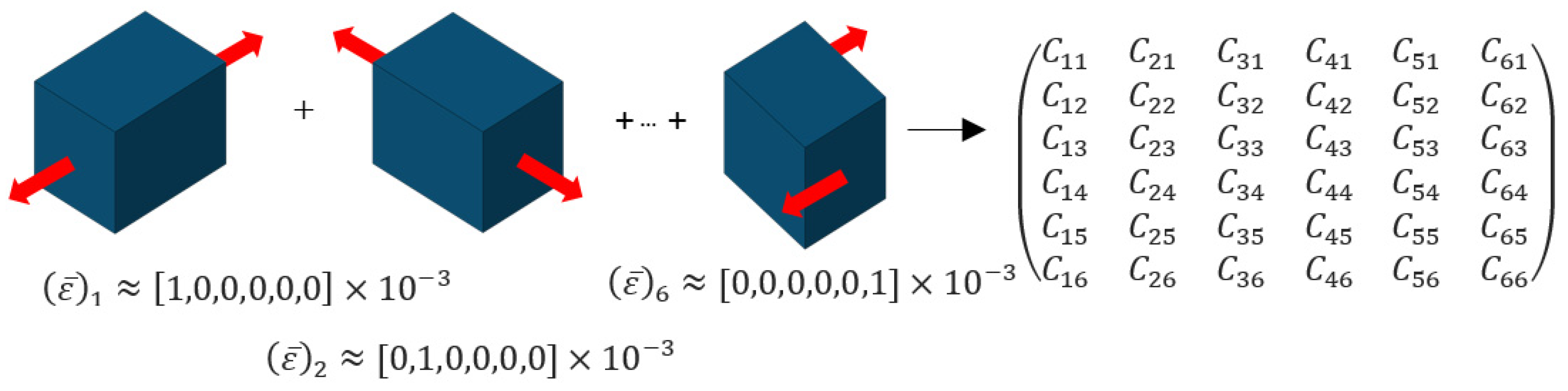
In this study, the complete effective stiffness tensor is to be used as a database, so that six independent simulations with different load directions must be performed with one RVE. Three tensile deformations and three shear deformations in each principal direction are carried out. For each simulation, , the stress and strain fields of the FEA are averaged by a homogenization scheme:
for the stress in direction and
for the strain . With the volume-averaged stresses from the six simulations, the effective stiffness tensor
is calculated. The procedure to determine the effective stiffness tensor is illustrated in Figure 1.
The effective stiffness tensor of one RVE depending on the input parameters of the creation represents a single data point of the database. As a first assumption, these individual data points should be distributed uniformly. For this reason, each input parameter for each RVE is randomly selected in an interval. The input parameters include the Young’s modulus and Poisson’s ratio of the matrix, the aspect ratio, the fiber volume fraction, and the second ordered fiber orientation tensor . To reduce the input parameters in this study only glass-fibers are considered. Therefore, the mechanical properties of the fibers are set to be constant with a Young’s Moduluse of 70,000 MPa and a Poisson’s ratio of 0.2. As beforementioned, the ODF is required for the rotation of the fibers within the volume of an RVE. Therefore, the ODF is reconstructed from the input parameter using the method of maximum entropy. Within this method a Bingham distribution is modified in such a way that the second order fiber orientation tensor calculated of the modified distribution corresponds to the given second order fiber orientation tensor. For more information, please refer to [22]. It must be noted that the normalization property of the fiber orientation tensor should be considered for the entries to distribute the possible fiber orientations properly. Independent random numbers for all three entries would lead to an overrepresentation of the isotropic case. Therefore, the entries are generated by
with
and
is a random variable, which is equally distributed between 0 and 1.
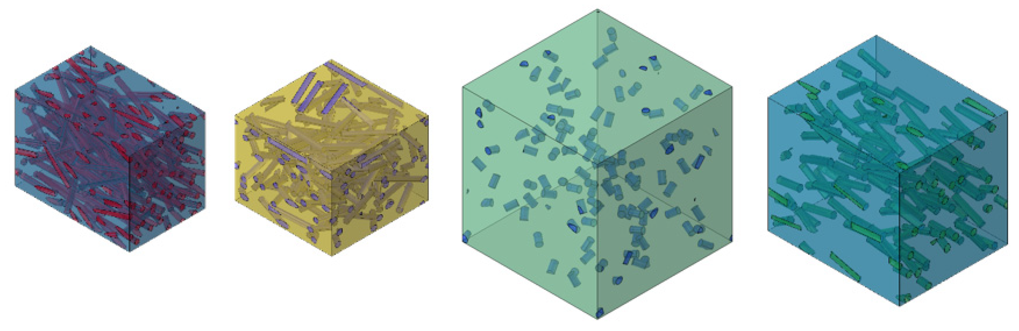
Figure 2 shows an example of 4 different RVEs with various input parameters. In this study, each RVE consist of 100 fibers. With different fiber volume fractions and aspect ratios and an identical number of fibers, the RVE’s volume can therefore be very different. However, based on preliminary tests by a convergence study, the used mesh size of the FEA is always identical. In the convergency study, the entries of the effective stiffness tensor show a maximum deviation of 1% from a converged reference solution. The used mesh size for this is 8 with a deviation factor of 0.1 and a minimum size factor of 0.1. The same mesh size and various volume sizes result in a very different number of elements. For example, with a low aspect ratio and high fiber volume fraction approximately 100,000 nodes per RVE are required but with a high aspect ratio and low fiber volume content about 4,000,000 nodes can be necessary. This also means that computing costs are different for each data point. Therefore, it might seem reasonable to prefer combinations of input parameters that results in lower computational effort, for example avoiding low volume fraction in combination with high aspect ratios. However, this conflicts with the reasonable demand for uniform distribution of data points. Therefore, this study evaluates if data sets must be distributed randomly or if they can be composed more favorable for cheaper data points to save computing time without loss of prediction quality of the neural network.
Within the scope of this investigation two datasets are generated, in which the input parameters are distributed uniformly as described but with different limits. With this division, it shall be shown that, for the elastic behavior of SFRP, a lot of computing time can be saved. Therefore, compared to the first dataset, in the second dataset the minimum fiber volume fraction is increased, as this is the parameter with the highest impact on computing time. Moreover, the two datasets demonstrate the case that an existing dataset is extended by one more input parameter. The considered case of expanding an existing dataset is thereby very important because the data set creation is extremely time-consuming. An extension of an existing data set would therefore offer an enormous time advantage for new investigations if less new data must be created. However, extending the data set has no direct benefit for this study, as it is one single study, but shows the possibility to reuse the data set in further studies, making the data creation much faster. In the first dataset, the Poisson’s ratio is set to a fixed value while in the second dataset the Poisson’s ratio is a random number. Table 1 summarizes the input parameters and lists the limits.
In Figure 3, all data points of the two datasets are shown as a correlation plot between each parameter pair. On the diagonal is also a histogram of the respective parameter. Both exclude a direct correlation between two input parameters per dataset due to an incorrect RVE creation. This would be recognizable here by empty regions in the correlation plots. Note that a uniform distribution of has a triangular shape, as they are not independent of each other. The differences between the two data sets are also visible in the figure. The constant Poisson’s ratio of dataset 1 can be seen, as well as the missing data points with a fiber volume fraction of less than 0.05 in dataset 2. A total of 1015 individual RVE’s are examined in total, 596 of which are contained in dataset 1 and 419 in dataset 2.
The next part of the section describes the neural network used. The implementation is carried out with Keras 2.3.1 [23] based on Tensorflow 1.14.
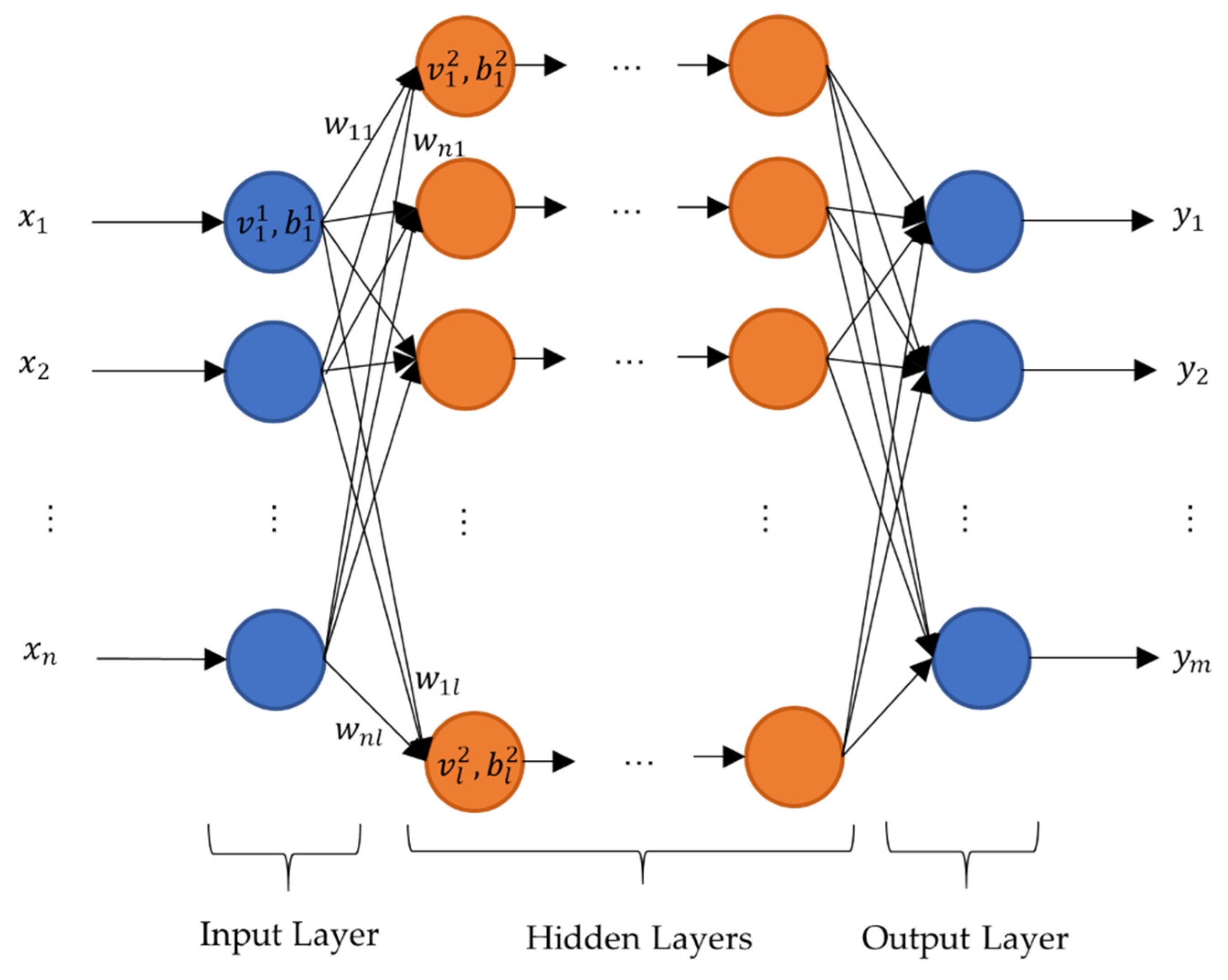
In general, a neural network consists of layers, each consisting of a set of neurons. Each neuron represents a numeric value . The number of neurons per layer can be different. The first layer is usually called the input layer with the input . Here the parameters for the creation of the RVEs are used as input parameters. The last layer is called the output layer with the output . Here the effective stiffness tensor of the RVEs is used as output. The layers in between are referred to as hidden layers. The hidden layers can be designed to be able to approximate any mathematical functions. The principal design is shown schematically in Figure 4. In this study, only dense layers are used. In dense layers the value of a neuron in one layer is linked to all neurons of the previous layer. The calculation of is done by an activation function with weights and [21,23]:
The weights and are also associated with a neuron. These weights can be fitted by numerical algorithms in such a way that a target function is minimized. This procedure is called training.
In this investigation, the “NAdam” algorithm [23] is used with the numerical parameters set to and . The mean square error between predictions and data provided by the RVEs is used as the target function [23]:
This target function is chosen to provide an average-based prediction. In Monte-Carlo simulations where only the position of the fibers within an RVE is varied, the calculated effective stiffness can be shown to be subject to statistical variation. This variation depends on the size of the RVE [24,25,26]. For the component design, however, a mean value of the effective stiffness is more appropriate. For this reason, the above-mentioned target function is used to train the neural network to an average value between the RVEs. To achieve training the average value, the architecture of the neural network must be suitable for this specific case, and overfitting must be avoided. Overfitting is referred to as the numerical behavior with which training data can be reproduced very well by the neural network, but new data cannot. A technique to check and control the overfitting is to split all data into training and validation data. Only the training data are used for the numerical adjustment of the weights. The evaluation of the target function is carried out for both separately.
In this study, all data are divided in the ratio ¾ into training data and ¼ into validation data. Furthermore, the division is performed randomly (for each data point) to create different sets of training and validation data if needed. All output is further normalized to the interval acc. to:
This step is necessary to treat the different entries of the stiffness tensor equally. Otherwise, the training could be favored for entries of higher stiffnesses such as the normal directions compared to other entries e.g., . For the input, it is not necessary.
As described in Section 2 the datasets 1 and 2 are used in combination. That means there is no separate evaluation for the two data sets. The objective of separate data sets is to be able to extend datasets. Therefore, a combined dataset is used.
In pre-trials the activation function was tested with
Here denotes a scalar and the input of a neuron. This function is referred to as “Elu” [23,27] and was found to be promising; hence, it is used for all hidden layers in this work. For input and output layers linear layers are used. For the input layer, 7 neurons are used according to the database for the input parameters , , , , , , . For the output, 9 neurons are used for the stiffness values , , , , , , , , . This reduction is justified based on symmetrical stiffness tensors and negligible tensile-shear coupling.
3. Results and Discussion
In this section the results are presented and discussed. This includes the development of an optimal structure of the neural network, accuracy of the neural network and a comparison with the classical method of Mori–Tanaka.
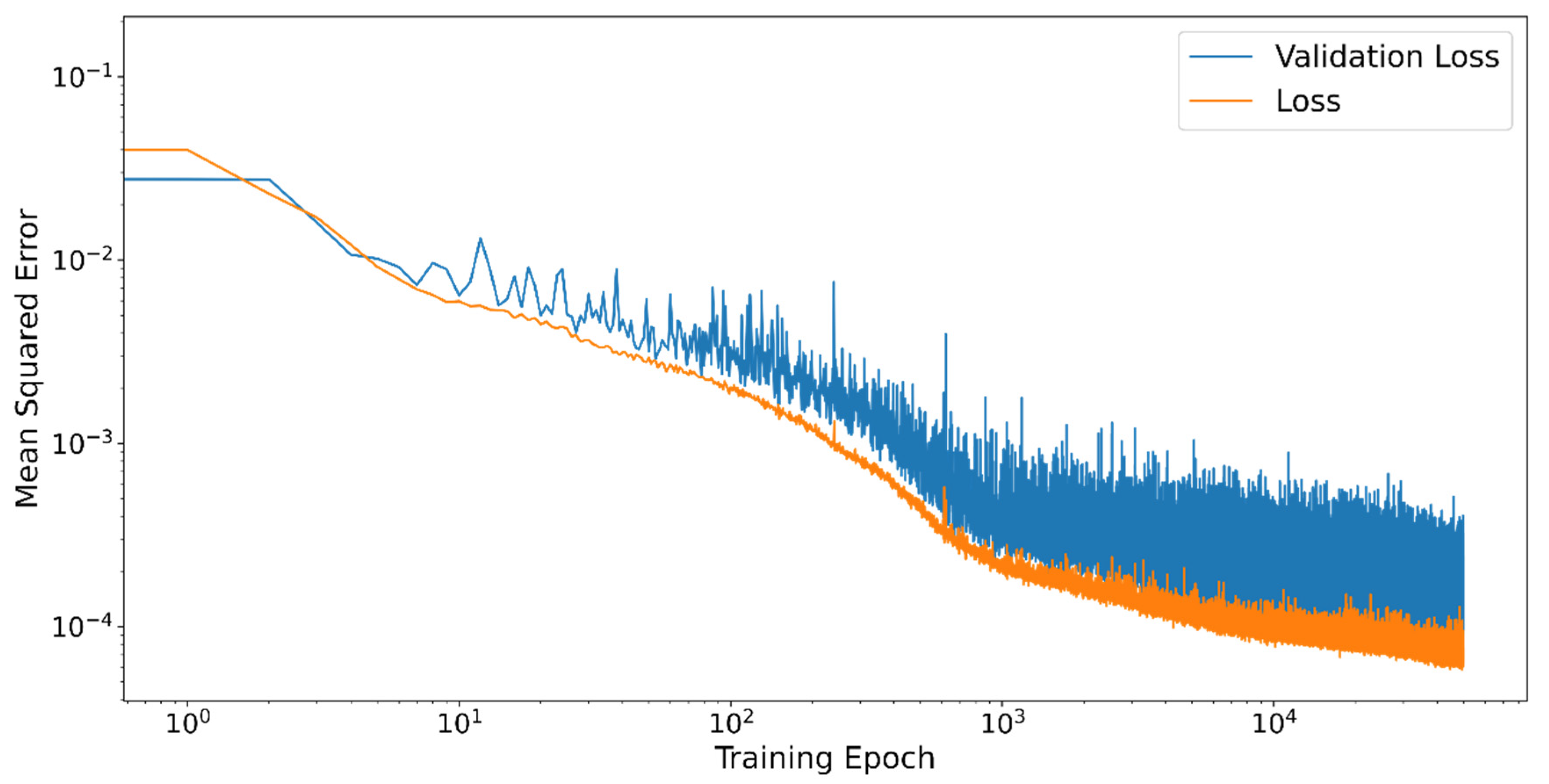
A typical training behavior for one layer and nine neurons is shown in Figure 5. The evaluations of the target function are plotted for the training data (Loss) and the validation data (Validation Loss) in double logarithmic order. From approximately epochs onwards the learning success becomes much more difficult and especially the Validation Loss is subject to strong fluctuations per epoch. Overfitting cannot be detected here.
In general, the neural network’s design is one of the most important factors in determining how it performs in terms of prediction accuracy, numerical robustness, and evaluation time. A neural network design with more layers and more neurons leads to a lower Loss and higher training time. If too many layers and neurons are used, overfitting may also be problematic. Therefore, a full factorial design of experiments (DOE) is performed to develop an optimal architecture of the neural network. The number of hidden layers is varied for 1, 2, 3, and 5 layers as well as the number of neurons per hidden layer with 9, 12, 15, and 18. A total of epochs are trained for each architecture. For the evaluation of the DOE, the epoch in which the absolute minimum of the Validation Loss is achieved is used. Due to the random division into training and validation data and the random initial weights [23], each neural network architecture is trained and evaluated for the DOE in a total repetition of 10. Figure 6 shows the result of the DOE as a boxplot of the minimum Validation Loss for each neural network architecture. Furthermore, each boxplot is color-coded with the average learning time per epoch. The training takes place on an Nvidia Tesla T4 16 GB.
For one and two layers it can be concluded that more neurons result in a lower minimum validation loss. With more layers, the number of neurons becomes less important. Furthermore, both the mean value and the variance of the minimum Validation Loss is significantly higher with one layer than with more layers. The conclusion is that with more layers the network becomes more robust and more accurate. Furthermore, it can be shown that here only the number of layers and not the number of neurons has a significant influence on the training time. In the later application with two hidden layers and 18 neurons, it is possible to calculate about 117,000 predictions per second with the neural network on an average PC (AMD Ryzen 3600 @ 4.1 GHz). For further investigation, an architecture of two hidden layers with 18 neurons each was used since it provides a low time of training and a low minimum Validation Loss. As a first evaluation, the validation data were compared with the predictions of the neural network. Furthermore, the predictions by a two-step homogenization are additionally performed to better judge the achieved accuracy of the neural network. The input parameters used for both methods are identical. In the first step of the two-step homogenization, the method of Mori–Tanaka is used [1]. A single ellipsoidal inclusion in a homogeneously stressed matrix is assumed. In the second step, the stiffness of the composite is composed of the stiffnesses for the individual directions of an ODF using the Voigt approach [28]. For the ODF, the method of maximum entropy [29] is used like for the creation of the RVEs (see Section 2). The neural network method is abbreviated with NN and the two-step homogenization with the Mori–Tanaka Method as MT in the following.
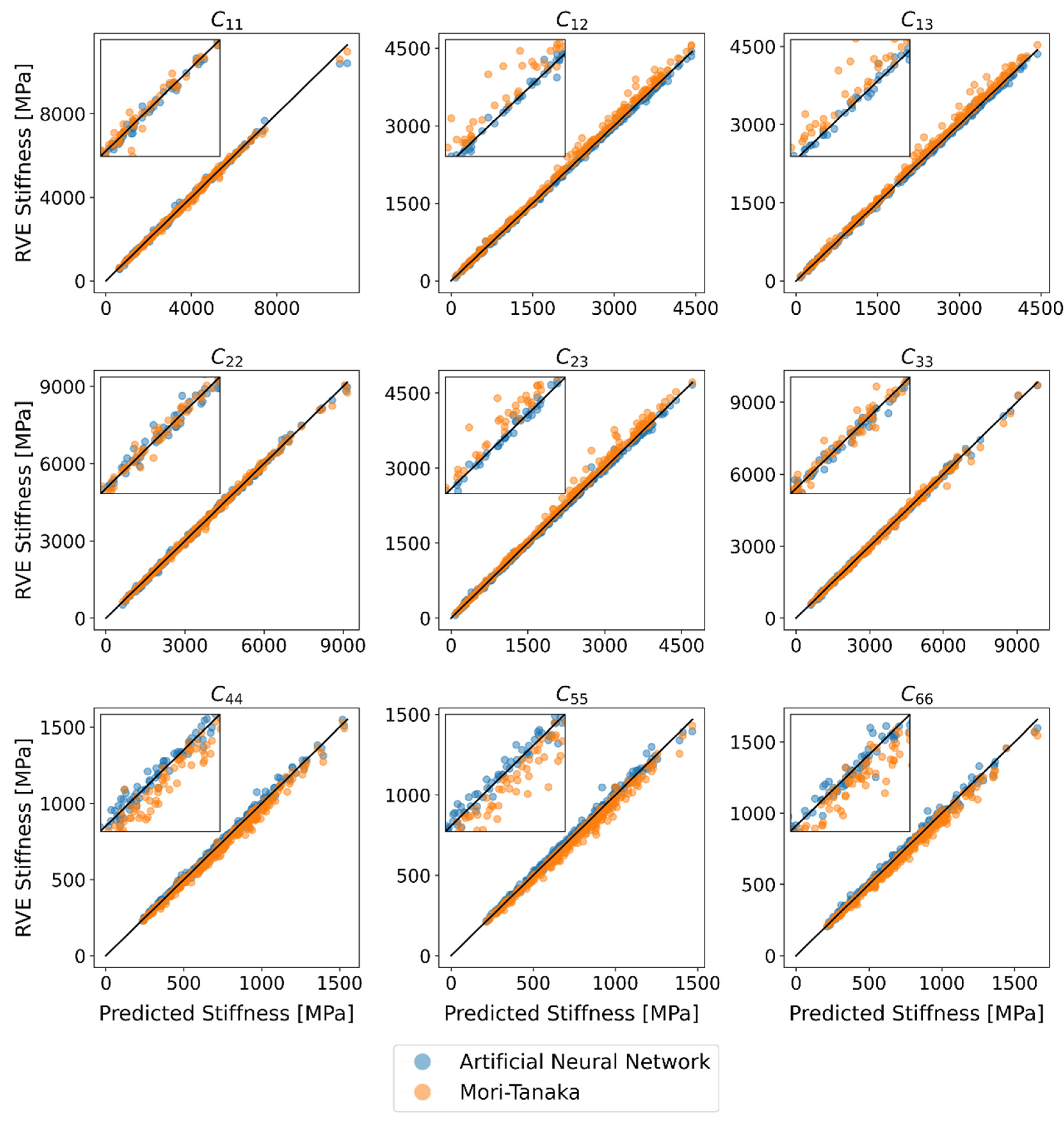
Figure 7 shows the predictions of NN and MT against the validation data. Ideally, the predictions would lie on one line. For better visibility of the data points, a small section from the center is shown enlarged. In general, it can be concluded that both NN and MT can reproduce the values of the RVE with a small error. Systematic errors, such as a greater deviation with higher stiffness, cannot be determined here for the NN.
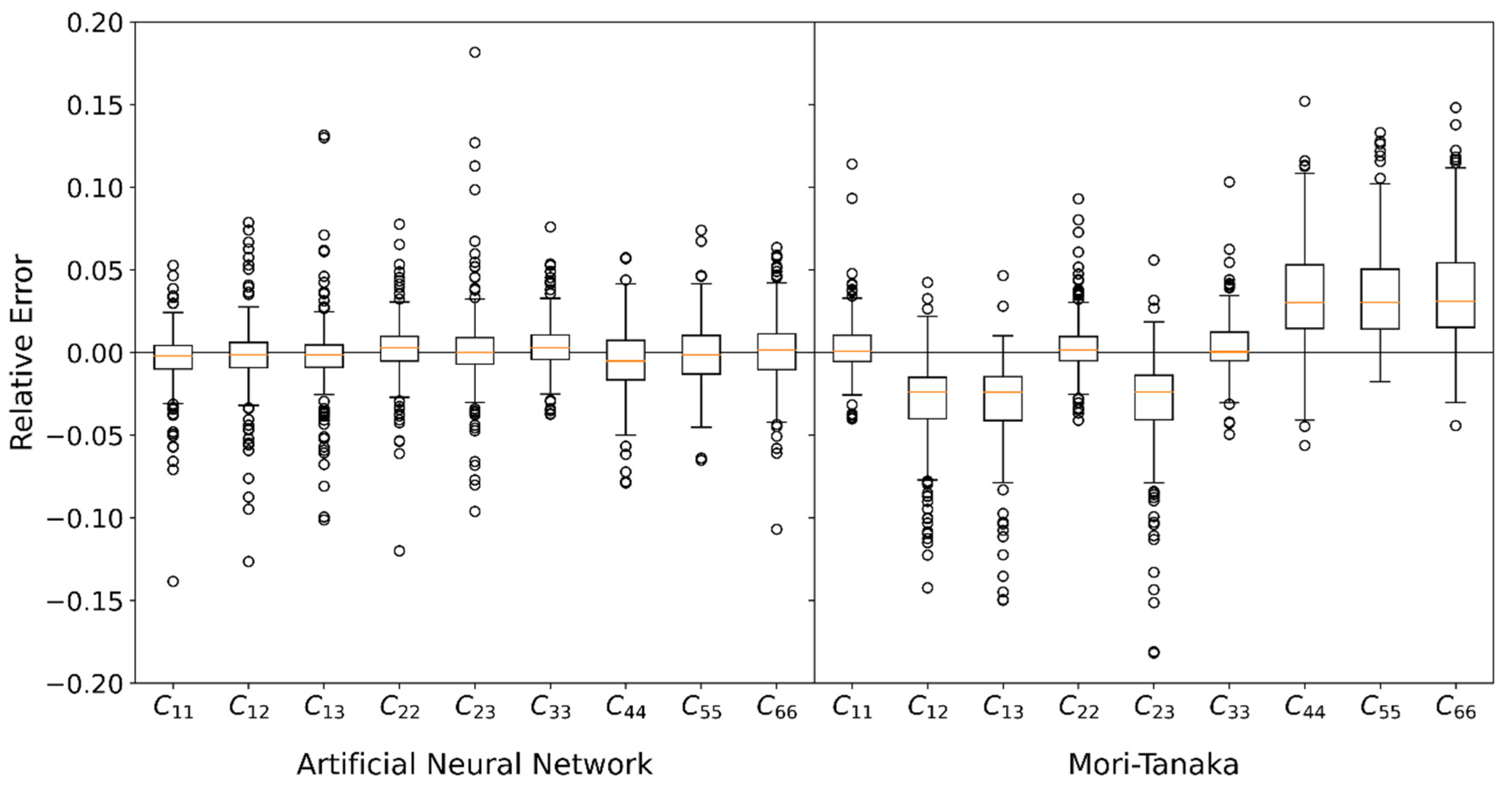
Further information about the accuracy of the NN in comparison with the MT method can be obtained in Figure 8. Here, for each stiffness entry a box plot with the relative error
is shown. is provided by the RVEs and only validation data are used.
With the NN method, the median of all relative errors is approximately zero, the interquartile distance is between 1.5% and 2.2%. Some outliers are in the range of 2.5% to 15 %. Note that the statistic distribution of relative errors is not only based on insufficient prediction, but also on the statistical deviation of the RVEs (see Section 2). Therefore, it can be concluded that NN is very well suited to predict the average stiffness of short fiber reinforced plastics.
With MT the absolute value of the mean error for the off-diagonal entries (, , ) and the shear entries (, , ) is approximately 3%. While the values are too high for the off-diagonal entries, they are too low for the shear entries. Moreover, the interquartile distances of 3.6–4.4% for the shear entries are significantly larger than those of the main entries (, , ) with 1.4–1.6%. As with the NN, the outliers also lie in a range from 5% to 20%. Comparing both methods with each other shows that the NN is on average more precise than the MT. Moreover, with the NN there is no systematic deviation for the median error. In normal directions, both methods perform similarly.
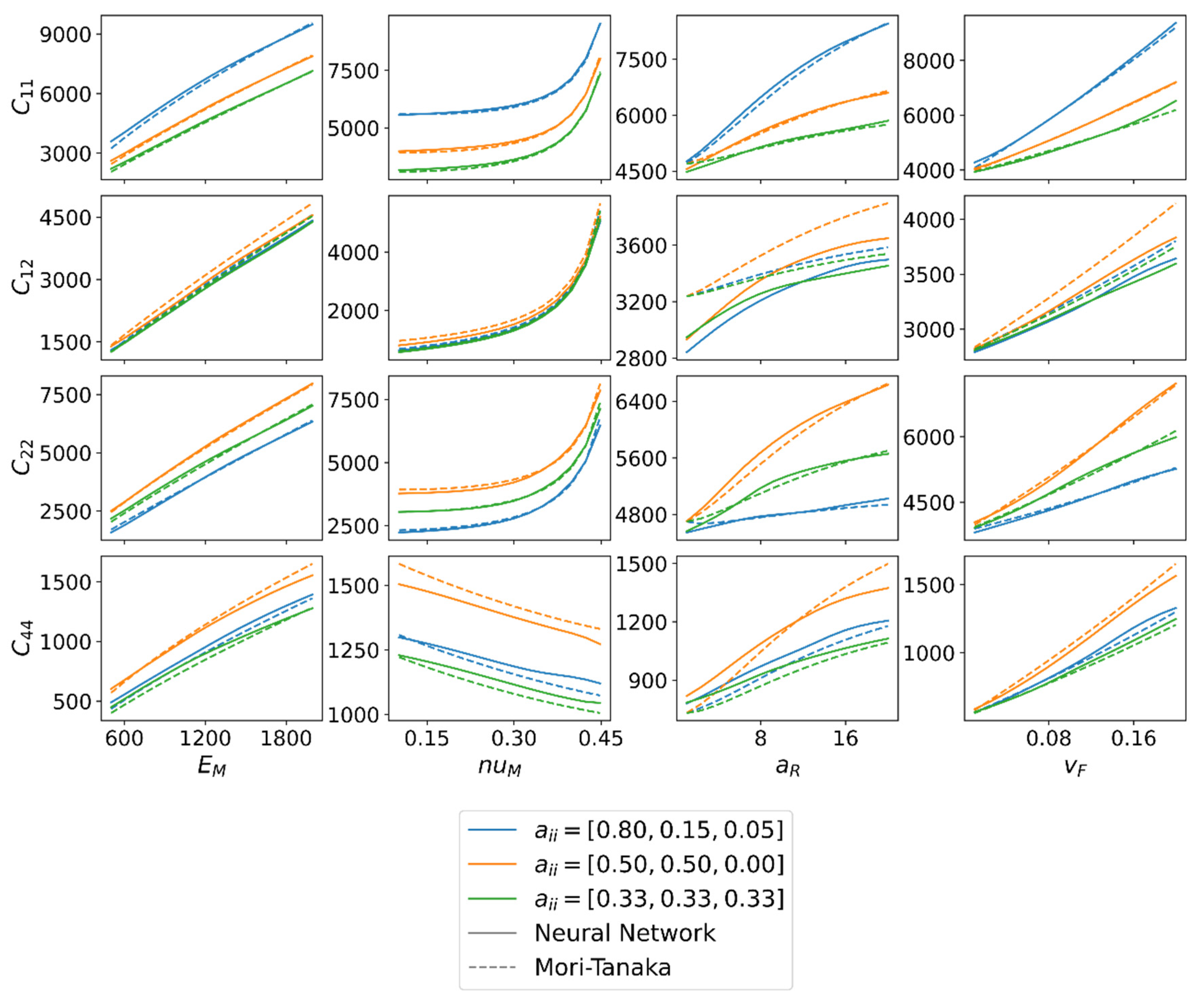
Figure 9 further clarifies the difference between predictions of NN and MT. A matrix of comparisons with the stiffness values (, , , ) in the rows and the input parameters (, , , ) in the columns is shown. These input parameters are constant for one entry of the matrix except that one which is varied in the associated column. The fiber orientation is chosen to be represented by three typical orientations (almost transversal isotropic, planar isotropic, and isotropic). The input parameters for the prediction are presented in Table 2.
Figure 9 shows that both methods provide almost identical predictions of the stiffness entry and for all input parameters. Larger differences can be observed for depending on the aspect ratio and the fiber volume fraction .
In both cases, the calculated stiffness value of MT is greater than that of NN. A possible explanation for the differences may be the assumptions of MT. On the one hand, the ellipsoid fiber geometry, especially with small aspect ratios, could lead to the deviation from the NN for . On the other hand, the assumption of homogeneous matrix stress is an explanation for the differences with increasing fiber volume content. However, it is interesting here that this is much more pronounced for off-diagonal entries than for the other stiffness entries. Further differences can be found in . Here, apart from , a difference can generally be found, usually with the higher values for the MT method. An exception is the prediction for aspect ratio with planar isotropic fiber orientation. Finally, the question of whether a combined dataset (cf. Section 2) is applicable can be answered. Neither in Figure 7 nor Figure 8 are systematic errors of the NN to be recognized. This indicates that no overfitting occurs at a Poisson’s ratio of 0.42 at the expense of other Poisson’s ratios. This is also supported by Figure 9, where the calculated values , and independent of the Poisson’s ratio do not deviate much from the MT. Only for the shear entry can larger deviations be recognized. However, these are more likely to be attributed to the general deviation (compared to the RVEs) of the MT prediction of . In addition, no statistically significant deviations of the NN can be found with a fiber volume fraction of less than 0.05. Therefore, it can be validated that an existing dataset can be extended by one more input parameter and numerically costly combinations of input parameters can be avoided if already enough data are available.
4. Conclusions
In this paper, an artificial neural network is developed and trained to predict the elastic properties of short fiber reinforced plastics. Representative volume elements are used as a data basis for this. For an input parameter field as wide as possible, Young’s modulus of the matrix, Poisson’s ratio of the matrix, aspect ratio, fiber volume fraction, and fiber orientation are varied.
With two separate data sets, it can be validated that an existing dataset can be extended by more input parameters without a loss of prediction accuracy. Moreover, it is shown that numerically costly combinations for the RVE creation can be avoided.
In principle, the prediction of the effective composite properties with the neural network is very accurate and robust. An optimal architecture of the neural network is found with 2 hidden layers, each with 18 neurons and an “Elu” activation function. The input and output layers are implemented with a linear activation function.
Compared to a two-step homogenization using the Mori–Tanaka method, the neural network performs equally () or slightly better () in calculating the mean elastic properties of short fiber-reinforced composites.
Furthermore, the evaluation shows a special strength of neural networks concerning material modeling: information on the micro-scale can be incorporated to make predictions more precise without generating uneconomical computational time on the macro-scale.
Author Contributions
Methodology, K.B., M.S.; software, K.B.; writing—original draft preparation, K.B.; writing—review and editing, M.S. supervision, M.S. All authors have read and agreed to the published version of the manuscript.
Funding
Funded by the Deutsche Forschungsgemeinschaft (DFG, German Research Foundation) STO 910/13-1.
Institutional Review Board Statement
Not applicable.
Informed Consent Statement
Not applicable.
Data Availability Statement
The data is not publicly available.
Conflicts of Interest
The authors declare no conflict of interest. The funders had no role in the design of the study; in the collection, analyses, or interpretation of data; in the writing of the manuscript, or in the decision to publish the results.
References
- Mori, T.; Tanaka, K. Average stress in matrix and average elastic energy of materials with misfitting inclusions. Acta Metall. 1973, 21, 571–574. [Google Scholar] [CrossRef]
- Hill, R. Elastic properties of reinforced solids: Some theoretical principles. J. Mech. Phys. Solids 1963, 11, 357–372. [Google Scholar] [CrossRef]
- Drugan, W.J.; Willis, J.R. A micromechanics-based nonlocal constitutive equation and estimates of representative volume element size for elastic composites. J. Mech. Phys. Solids 1996, 44, 497–524. [Google Scholar] [CrossRef]
- Gitman, I.M.; Askes, H.; Sluys, L.J. Representative volume: Existence and size determination. Eng. Fract. Mech. 2007, 74, 2518–2534. [Google Scholar] [CrossRef]
- Sun, C.T.; Vaidya, R.S. Prediction of composite properties from a representative volume element. Compos. Sci. Technol. 1996, 56, 171–179. [Google Scholar] [CrossRef]
- Feyel, F. Multiscale FE2 elastoviscoplastic analysis of composite structures. Comput. Mater. Sci. 1999, 16, 344–354. [Google Scholar] [CrossRef]
- Liu, Z.; Wu, C.T.; Koishi, M. A deep material network for multiscale topology learning and accelerated nonlinear modeling of heterogeneous materials. Comput. Methods Appl. Mech. Eng. 2019, 345, 1138–1168. [Google Scholar] [CrossRef] [Green Version]
- Chen, G.; Wang, H.; Bezold, A.; Broeckmann, C.; Weichert, D.; Zhang, L. Strengths prediction of particulate reinforced metal matrix composites (PRMMCs) using direct method and artificial neural network. Compos. Struct. 2019, 223, 110951. [Google Scholar] [CrossRef]
- Rao, C.; Liu, Y. Three-dimensional convolutional neural network (3D-CNN) for heterogeneous material homogenization. Comput. Mater. Sci. 2020, 184, 109850. [Google Scholar] [CrossRef]
- Yang, C.; Kim, Y.; Ryu, S.; Gu, G.X. Prediction of composite microstructure stress-strain curves using convolutional neural networks. Mater. Des. 2020, 189, 108509. [Google Scholar] [CrossRef]
- Jung, S.; Ghaboussi, J. Neural network constitutive model for rate-dependent materials. Comput. Struct. 2006, 84, 955–963. [Google Scholar] [CrossRef]
- Zhang, A.; Mohr, D. Using neural networks to represent von Mises plasticity with isotropic hardening. Int. J. Plast. 2020, 132, 102732. [Google Scholar] [CrossRef]
- Rocha, I.B.C.M.; Kerfriden, P.; van der Meer, F.P. Micromechanics-based surrogate models for the response of composites: A critical comparison between a classical mesoscale constitutive model, hyper-reduction and neural networks. Eur. J. Mech. A Solids 2020, 82, 103995. [Google Scholar] [CrossRef]
- Wu, L.; van Nguyen, D.; Kilingar, N.G.; Noels, L. A recurrent neural network-accelerated multi-scale model for elasto-plastic heterogeneous materials subjected to random cyclic and non-proportional loading paths. Comput. Methods Appl. Mech. Eng. 2020, 369, 113234. [Google Scholar] [CrossRef]
- Ghavamian, F.; Simone, A. Accelerating multiscale finite element simulations of history-dependent materials using a recurrent neural network. Comput. Methods Appl. Mech. Eng. 2019, 357, 112594. [Google Scholar] [CrossRef]
- Settgast, C.; Hütter, G.; Kuna, M.; Abendroth, M. A hybrid approach to simulate the homogenized irreversible elastic–plastic deformations and damage of foams by neural networks. Int. J. Plast. 2019, 102624. [Google Scholar] [CrossRef] [Green Version]
- Settgast, C.; Abendroth, M.; Kuna, M. Constitutive modeling of plastic deformation behavior of open-cell foam structures using neural networks. Mech. Mater. 2019, 131, 1–10. [Google Scholar] [CrossRef]
- Gorji, M.B.; Mozaffar, M.; Heidenreich, J.N.; Cao, J.; Mohr, D. On the potential of recurrent neural networks for modeling path dependent plasticity. J. Mech. Phys. Solids 2020, 143, 103972. [Google Scholar] [CrossRef]
- Zhang, X.; Garikipati, K. Machine learning materials physics: Multi-resolution neural networks learn the free energy and nonlinear elastic response of evolving microstructures. Comput. Methods Appl. Mech. Eng. 2020, 372, 113362. [Google Scholar] [CrossRef]
- Matos, M.A.S.; Pinho, S.T.; Tagarielli, V.L. Predictions of the electrical conductivity of composites of polymers and carbon nanotubes by an artificial neural network. Scr. Mater. 2019, 166, 117–121. [Google Scholar] [CrossRef]
- Matos, M.A.S.; Pinho, S.T.; Tagarielli, V.L. Application of machine learning to predict the multiaxial strain-sensing response of CNT-polymer composites. Carbon 2019, 146, 265–275. [Google Scholar] [CrossRef]
- Breuer, K.; Stommel, M. RVE Modelling of Short Fiber Reinforced Thermoplastics with Discrete Fiber Orientation and Fiber Length Distribution. SN Appl. Sci. 2020, 2, 91. [Google Scholar] [CrossRef] [Green Version]
- Chollet, F. Keras. 2015. Available online: https://keras.io (accessed on 26 January 2021).
- Kanit, T.; Forest, S.; Galliet, I.; Mounoury, V.; Jeulin, D. Determination of the size of the representative volume element for random composites: Statistical and numerical approach. Int. J. Solids Struct. 2003, 40, 3647–3679. [Google Scholar] [CrossRef]
- Hazanov, S.; Huet, C. Order relationships for boundary conditions effect in heterogeneous bodies smaller than the representative volume. J. Mech. Phys. Solids 1994, 42, 1995–2011. [Google Scholar] [CrossRef]
- Huet, C. Application of variational concepts to size effects in elastic heterogeneous bodies. J. Mech. Phys. Solids 1990, 38, 813–841. [Google Scholar] [CrossRef]
- Clevert, D.-A.; Unterthiner, T.; Hochreiter, S. Fast and Accurate Deep Network Learning by Exponential Linear Units (ELUs), 2015. ICLR 2016, 5, 1–14. Available online: http://arxiv.org/pdf/1511.07289v5 (accessed on 26 January 2021).
- Voigt, W. Ueber die Beziehung zwischen den beiden Elasticitätsconstanten isotroper Körper. Ann. Phys. 1889, 274, 573–587. [Google Scholar] [CrossRef] [Green Version]
- Breuer, K.; Stommel, M.; Korte, W. Analysis and Evaluation of Fiber Orientation Reconstruction Methods. J. Compos. Sci. 2019, 3, 67. [Google Scholar] [CrossRef] [Green Version]
Figure 1.
Illustration of combined deformations to determine complete stiffness tensor.

Figure 2.
Illustration of four representative volume elements (RVEs) (each with 100 fibers) with different random parameters of the microstructure.
Figure 2.
Illustration of four representative volume elements (RVEs) (each with 100 fibers) with different random parameters of the microstructure.

Figure 3.
Correlation plot between all parameters of the RVE’s for two different input datasets. Dataset 1 features a constant Poisson’s ratio of the matrix material and Dataset 2 has a higher minimum fiber volume fraction.
Figure 3.
Correlation plot between all parameters of the RVE’s for two different input datasets. Dataset 1 features a constant Poisson’s ratio of the matrix material and Dataset 2 has a higher minimum fiber volume fraction.

Figure 4.
Schematic design of neural network with dense layers.

Figure 5.
Training behavior of the neural network for each training epoch. The neural network is evaluated by the objective function for the training data (Loss) and the validation data (Validation Loss).
Figure 5.
Training behavior of the neural network for each training epoch. The neural network is evaluated by the objective function for the training data (Loss) and the validation data (Validation Loss).

Figure 6.
Boxplot of minimum Validation Loss and mean training time per epoch for each architecture.
Figure 6.
Boxplot of minimum Validation Loss and mean training time per epoch for each architecture.

Figure 7.
Comparison between Stiffness by RVE and Stiffness predictions by the neural network method (NN) and Mori–Tanaka Method (MT).
Figure 7.
Comparison between Stiffness by RVE and Stiffness predictions by the neural network method (NN) and Mori–Tanaka Method (MT).

Figure 8.
Boxplot of relative Error by NN and MT.

Figure 9.
Direct comparison between model predictions of NN and MT for different input parameters. All input parameters are constant (see Table 2) except that one which is varied in the associated column.
Figure 9.
Direct comparison between model predictions of NN and MT for different input parameters. All input parameters are constant (see Table 2) except that one which is varied in the associated column.


Table 1.
Range of the parameters of the two datasets.
| Parameter | Dataset 1 | Dataset 2 |
|---|---|---|
| 500–2000 MPa | 500–2000 MPa | |
| 0.42 | 0.1–0.45 | |
| 1–20 | 1–20 | |
| 0.01–0.2 | 0.05–0.2 | |
| 0–1 | 0–1 |
Table 2.
Input parameter for the prediction.
| Parameter | Constant Value |
|---|---|
| 1500 MPa | |
| 0.42 | |
| 15 | |
| 0.15 | |
| 0.8, 0.5 and 0.33 | |
| 0.15, 0.5 and 0.33 | |
| 0.05, 0.0 and 0.33 |
Publisher’s Note: MDPI stays neutral with regard to jurisdictional claims in published maps and institutional affiliations. |
© 2021 by the authors. Licensee MDPI, Basel, Switzerland. This article is an open access article distributed under the terms and conditions of the Creative Commons Attribution (CC BY) license (http://creativecommons.org/licenses/by/4.0/).
Share and Cite
MDPI and ACS Style
Breuer, K.; Stommel, M. Prediction of Short Fiber Composite Properties by an Artificial Neural Network Trained on an RVE Database. Fibers 2021, 9, 8. https://0-doi-org.brum.beds.ac.uk/10.3390/fib9020008
AMA Style
Breuer K, Stommel M. Prediction of Short Fiber Composite Properties by an Artificial Neural Network Trained on an RVE Database. Fibers. 2021; 9(2):8. https://0-doi-org.brum.beds.ac.uk/10.3390/fib9020008
Chicago/Turabian StyleBreuer, Kevin, and Markus Stommel. 2021. "Prediction of Short Fiber Composite Properties by an Artificial Neural Network Trained on an RVE Database" Fibers 9, no. 2: 8. https://0-doi-org.brum.beds.ac.uk/10.3390/fib9020008
Note that from the first issue of 2016, this journal uses article numbers instead of page numbers. See further details here.