Multiproduct Economic Lot Scheduling Problem with Returns and Sorting Line


Department of Mechanical and Industrial Engineering, University of Brescia, Via Branze, 38-25123 Brescia, Italy
Systems 2020, 8(2), 16; https://0-doi-org.brum.beds.ac.uk/10.3390/systems8020016
Submission received: 18 March 2020
/
Revised: 18 April 2020
/
Accepted: 20 May 2020
/
Published: 26 May 2020
(This article belongs to the Special Issue Industry 4.0 and Energy-Efficient Production Planning)
Abstract
:This work studies a hybrid manufacturing–remanufacturing system with a sorting line and disposal. In particular, it models a company that collects used product, remanufactures returned products that have been evaluated as suitable to be recovered, and manufactures new products to satisfy customer demand. Specifically, the system is modeled as a multilevel inventory system, with three types of stock (used products inventory, recoverable inventory, and serviceable inventory), each characterized by an inventory holding cost, and three limited capacity resources: a sorting line, which enables the company to distinguish those returns that are remanufacturable from those that are not; a remanufacturing line to carry out operations on sorted remanufacturable returns; and a manufacturing line to produce new products in order to satisfy customer demand. Each resource is characterized by a setup cost, as well as a constant production rate, while each type of stock is associated with an inventory holding cost. The aim of the paper is to develop a model for the considered production system in order to minimize the setup and inventory holding costs. In particular, the objective is to evaluate the behavior of a controllable disposal rate with the minimization of the total cost function, by considering the effect on the remanufacturing and manufacturing lines.
1. Introduction
In recent years, the reuse of products and materials has been given increasing attention due to (1) the increasing environmental sensibilization of producers and consumers, (2) the development of specific environmental legislation based on the reuse of products and materials at the end of their life cycle, (3) the possibility of making a profit from the management of the reverse flow in the supply chain. In this last case, the profitability is based on the possibility of making the reused products or materials as good as new. This situation introduces remanufacturing systems and the production and inventory problems connected to the management of manufacturing and remanufacturing resources. In fact, the demand for final products typically outweighs returns, so it is necessary to use both types of resources.
In this system it is possible to include a disposal option, whereby the reused products are controlled and eventually discarded before starting the remanufacturing process. The disposal option makes the system more difficult to control and analyze, but may lead to a cost reduction [1]. In fact, the disposal option will lead to a reduction in the number of returned products because many will not be of the quality necessary to obtain a good-as-new product [2] after the remanufacturing process. In general, in this kind of system the disposal options are executed in a sorting line, which enables the company to distinguish those returns that are remanufacturable from those that are not. Obviously, it is necessary to consider the costs related to the sorting line and the effect on the total costs of the system of the disposal options. The objective of this research is to consider the sorting line in the hybrid manufacturing–remanufacturing schema in order to optimize the lot sizing of the different operations by minimizing the production costs (setup and inventory). In particular, to minimize the total production costs, it is important to evaluate the effects of the disposal percentage (i.e., the percentage of returned products that are disposed of and thus do not proceed through the remanufacturing process) with respect to the utilization of the limited c resources involved in the system.
The economic lot scheduling problem with returns (ELSPR), introduced by [3], arises from the need to accommodate several items in production at once by undertaking manufacturing and remanufacturing operations on returned items on a single line, with the goal of minimizing the total setup and holding costs.
The ELSPR model is based on the ELSP model developed by [4], who identified the need for scheduling items at a single production center in order to minimize the total setup and holding costs by defining their Economic Lot Quantity (ELQ). Ref. [5] described a system wherein EOQ-type formulations (Economic Order Quantity) were used for controlling repairable inventories, which has to do with what was later defined as the ELSP problem “with returns”.
Ref. [6] proposed an EOQ-type formula for this kind of problem, presuming a fixed cost for manufacturing and remanufacturing lots, as well as inventory holding costs for repairable and newly manufactured products. Ref. [7,8,9] presented EOQ repair and waste disposal models with variable setup numbers n and m for production and repair, respectively. A share of the used products is collected and later repaired; the other products are disposed of. Meanwhile, some collection time intervals are considered. The goal is the minimization of the total cost function. Ref. [10,11] investigated a production–recycling system. A constant demand can be satisfied by production and recycling. The used items are bought back and then recycled. The nonrecycled products are disposed of. Two types of models have been analyzed. The first model examines the EOQ-related costs and minimizes the relevant costs. The second model generalizes the first model with the introduction of the cost function with linear waste disposal, recycling, production, and buyback costs.
Ref. [12] studied a deterministic EOQ model of an inventory system with items that can be recovered (repaired/refurbished/remanufactured). He used different holding cost rates for manufactured and recovered items and included disposal. He derived simple square root EOQ formulas for both the manufacturing batch quantity and the recovery batch quantity. Then, ref. [13] analyzed inventory systems with product recovery. Recovered items are as good as new and satisfy the same demands as new items. The demand rate and return fraction are deterministic. The relevant costs are those for ordering recovery lots, for ordering production lots, for holding recoverable items in stock, and for holding new/recovered items in stock. He derived simple formulae that determine the optimal lot sizes for the production/procurement of new items and for the recovery of returned items. These formulae are valid for finite and infinite production and recovery rates.
Ref. [1] studied a single item hybrid production system with manufacturing and remanufacturing. They assumed that remanufacturing is profitable and that, on average, there is more demand than there are returns. They investigated, using a simulation, how the cost changes when having a disposal option for returned items. Ref. [14] modeled a hybrid system whereby the remanufactured and manufactured items are managed separately at the serviceable inventory level and the component inventory control decisions are coordinated; in their model, the control of the remanufacturable and new component inventories is through the control of disposal and new component order: such decisions are based on the total system costs. Also, ref. [15] suggested that returned products from customers could be kept in remanufacturable inventory, but only a portion of them will be remanufactured and the rest will be disposed of. Ref. [16] observed that, when the conditions of the collected used products are variable, remanufacturing them could be more expensive than disposing of them: this implies that the number of used products acquired should be greater than the number of remanufactured products required. The result is a remanufacturing “yield,” defined as the percentage of the used products acquired that are actually remanufactured; the firm acknowledges that increasing selectivity in its sorting (i.e., accepting fewer products for remanufacturing) will have two effects: (1) yield will decrease, requiring the acquisition of more used products to meet the demand, and (2) the remanufacturing cost will decrease since the used products sorted for remanufacturing will be, on average, in better condition.
Ref. [17] proposed two procedures to find the optimal lot sizing solution in a deterministic scenario remanufacturing system, and three solution procedures for the related stochastic scenario environment. One of the main goals of their work was to determine the optimal solution assessment of manufacturing and remanufacturing lots, where a constant demand of components has to be satisfied over an infinite planning horizon in a cyclic pattern.
Ref. [18] proposed a mathematical model for the ELSP with reworks using the common cycle approach in which only one manufacturing lot and only one rework lot for each product exist during a common cycle. In order to solve this problem, they proposed two heuristics that not only search for the optimal cycle time and an optimal production sequence, but also utilize a simple scheduling heuristic to schedule the starting time of all the manufacturing and rework lots so as to minimize the average total cost. In [19], production, remanufacture, and waste disposal EPQ (economic production quantity) type models are developed and analyzed, where a manufacturer serves a stationary demand by producing new items as well as remanufacturing collected used/returned items. Regarding disposal operations related to production/remanufacturing systems, ref. [20,21] proposed a model considering production, remanufacturing, and disposal operations; they showed when and why systems with planned disposal (disposal of items that are in principle remanufacturable) are economically more efficient than systems in which no planned disposal occurs.
Ref. [3] minimized the average total cost by optimizing the acquisition lot size and scheduling the remanufacturing sequence. First, they scheduled the remanufacturing sequence for an independent remanufacturing system, and subsequently extended the model to a hybrid manufacturing–remanufacturing system. The benefit of scheduling the remanufacturing sequence is the low holding cost for storing returns and postponing the remanufacturing process to when they are needed.
Ref. [22], by relaxing the constraint of common cycle time and a single (re)manufacturing lot for each item in each cycle, proposed a simple, easy-to-implement algorithm, based on [23], to solve the model using a basic period policy.
Ref. [24] modeled the Economic Lot Scheduling problem with returns (ELSPR) under the basic period (BP) policy with power-of-two (PoT) multipliers, and solved it with a discrete artificial bee colony (DABC) algorithm. The numerical study suggests that the proposed algorithm performs well under the BP–PoT policy and has the potential of improving the best-known solutions when we relax BP, PoT, and independently managed serviceable inventory restrictions in the future.
In this work the role of controllable disposal is investigated, extending the work of [21] to the ELSPR problem. Moreover, as presented in [16], the number of used products acquired should be greater than the number of remanufactured products required: this result is a remanufacturing “yield,” defined as the percentage of the used products acquired that are actually remanufactured. The problem is formulated as a multi-item ELSPR problem, with multiple limited-capacity manufacturing/remanufacturing resources, as proposed by [25,26], and also an inspection/sorting process on a further limited capacity resource, extending the work of [27]. Table 1 summarizes the main assumptions of the present work, indicating the previous contributions. In our opinion, the literature offers only partial solutions to the problem addressed in this work, which also proposes the extension of the ELSPR methodology to a hybrid manufacturing–remanufacturing system with a sorting line and disposal option.
2. Problem Definition
A company that collects used product, remanufactures returned products that have been evaluated as suitable to be recovered, and manufactures new products to satisfy customer demand is the background for the problem setting. The system is modeled as a multilevel inventory system, with three stages (Returned products inventory—U, Recoverable inventory—R, Serviceable inventory—S) and three limited capacity resources (Sorting Line—SL, Remanufacturing Line—RL, Manufacturing Line—ML).
The focus is on a certain number of items, which are collected in the first stock, named the Returned products inventory (U); then all products are sorted in the first system resource, the Sorting Line (SL), to distinguish “remanufacturable” returns from those that are not; these are then sent to the disposal system, while the others are first stocked by the Recoverable inventory (R) and then remanufactured on what we name the Remanufacturing Line (RL); after remanufacturing operations, remanufactured products are stored by the Serviceable inventory (S), together with newly manufactured products made on the Manufacturing Line (ML), before being sold on the market. Remanufacturing operations make remanufactured returns “as good as new.” Figure 1 shows the system main flows.
The customer demand for final products is assumed to be constant and depletes the finished goods inventory (S) continuously by a constant rate of Di units per time unit (index i denotes item i). In order to satisfy that demand, the company manufactures the final product.
When a customer has no further use for an item or product, s/he has the opportunity to return it to the company: as the return rate βi depends on the customer’s decision to give back the useless item to the company, the fraction βiDi of the products in the market usually is not constant over time, even if we can say that it depends on the demand rate Di, which is supposed to be constant over time; thus, we assume that both βi and Di are deterministic and constant over time.
After their arrival at the Returned products inventory (U), which is continuously filled by a returned rate βiDi of products, returns have to be examined, in order to verify the possibility of remanufacturing them. These operations are performed by the Sorting line (SL) resource: non remanufacturable returns are sent to the disposal system; otherwise, they fill the Recoverable inventory (R) after a sorting process time, which depends on the return rate βiDi and the sorting rate (psi) of the resource, for the considered item i. The remanufacturable returns percentage is denoted λi, so that the flow of items reaching the Recoverable inventory can be denoted λiβiDi; accordingly, (1λi)βiDi represents the disposal rate. The Remanufacturing line (RL) empties the Recoverable inventory and, after a remanufacturing process time, fills the Serviceable inventory (S). In order to satisfy customer demand, it is necessary that the Serviceable inventory “emptying rate” equals the demand rate Di: this means that the Manufacturing line (ML) fills the Serviceable inventory at a rate of (1 − λiβi)Di, which is the disposal rate increased by the “nonreturn” rate (1 − βi)Di, as reported in the following:
- Disposal rate: (1 − λi)βiDi (for all i).
- “Nonreturn” rate: (1 − βi)Di (for all i).
- (1 − λi)βiDi + (1 − βi)Di = (1 − λiβi)Di (for all i).
All sorting, manufacturing, and remanufacturing operations should be scheduled during the cycle time T, which is common for all the production lines (SL, ML, and RL).
The flow of items reaching the Recoverable inventory, denoted as λiβiDi, usually involves a certain utilization of the Remanufacturing line RL, and consequently of the Manufacturing line ML: one of the objectives of this work is to consider a controllable disposal rate that can allow the minimization of the total cost of the whole production system. That means that the value of the parameter λi is the one allowing such a cost minimization. In fact, remanufacturing all the items that have been evaluated as suitable for that kind of operation is usually less profitable than disposing of a certain amount of them and producing a new product on the ML; the choice of how much to dispose of (and so how much to manufacture and remanufacture) influences the utilization of the two production lines. The amount of returns that have been evaluated as suitable for remanufacturing operations is usually quite high (as the collection of returns itself involves a selection of items), so it should be possible to decide to dispose of a certain quantity of returns and accept for remanufacturing operations only a lower rate λiβiDi (which will flow into the Recoverable inventory), where λi has to be determined with the aim of minimizing the total cost of the whole system, also considering the costs related to the production of new products on ML.
As it is proven that more value is added to the components on each inventory level, holding costs are connected by the following inequality, when considering a three-level inventory system: holding costfirst_level < holding costsecond_level < holding costthird_level, which means that for the considered system we assume that hui < hri < hsi (for all item i). A detailed discussion of how to set holding cost parameters can be found in [28].
In order to improve the system performance in terms of holding costs, we should assume that the Serviceable inventory (S), related to item i, is filled only by one production line (RL or ML) at a time: this can avoid extra holding costs related to filling the Serviceable inventory with a lot of item i worked out by RL (or ML) when its inventory level is not zero.
In order to configure a system based on the optimality of related costs, the following assumptions should be considered:
- If the Remanufacturing Line (RL) is performing operations on item i, the Manufacturing Line (ML) is performing operations on a different item j, in order to fill the Serviceable inventory (S) only with lots of item i worked out by RL or by ML (not from both lines simultaneously). It should also be specified that it is not necessary that at any time some items i should come to S: it is only requested that during the cycle time T, demand Di is satisfied for all items at any time.
- When the production of item i is scheduled on RL and ML, it should be considered that the time spent for operations on RL and ML, together with the time spent for consuming the produced quantity (emptying the Serviceable inventory), should be equal to cycle time T.
Fixed and holding costs can be balanced by applying an average cost approach to the model. This is common for one-level as well as multilevel inventory systems, adopting the well-known EOQ-model formulation and respecting its assumptions (infinite planning horizon with constant costs over time). As a result, an optimal cyclic pattern can be obtained by minimizing the average cost per time unit.
In order to control the system, a certain number of decision variables are required for each item kind, including frequency values on the three production lines, and, most important, the cycle length T value must be determined as a common value for the three lines for all items.
3. Model Formulation
In this section, a model that allows for the evaluation of the optimal time dedicated to sorting, remanufacturing, and manufacturing operations during a cycle time T is introduced.
3.1. Notation
The following notation is used throughout the paper:
| N | number of items |
| i | item index |
| Di | demand rate for item i in units per unit time (production days) |
| βi | return rate of item i (percentage) |
| (1 − λi) | controllable disposal rate of item i (λi is the percentage of returned products that are selected for remanufacturing operations) |
| psi | production rate of item i on the Sorting Line (SL) |
| pri | production rate of item i on the Remanufacturing Line (RL) |
| pmi | production rate of item i on the Manufacturing Line (ML) |
| s | setup time (time units) for any production lines, for any item lot |
| hui | inventory holding cost of item i for Returned products inventory (U) per unit and time unit |
| hri | inventory holding cost of item i for Recoverable inventory (R) per unit and time unit |
| hsi | inventory holding cost of item i for Serviceable inventory (S) per unit and time unit |
| Ai | setup cost for any production lines, for each lot of item i |
| T | cycle time length (in time units) |
| fiSL | production frequency of item i on Sorting Line (number of lots of item i worked out by SL) |
| fiRL | production frequency of item i on Remanufacturing Line (number of lots of item i worked out by RL) |
| fiML | production frequency of item i on Manufacturing Line (number of lots of item i worked out by ML). |
Moreover, the following main assumptions are adopted for the development of the model:
Equation (1) assures that the Serviceable inventory (S) follows the typical saw-tooth pattern, as it will be detailed in the next paragraph, while Equations (2)–(4) ensure that setup times do not interfere with any production activities. Equations (5)–(10) define the time slots.
3.2. The Total Cost Function
Returned products inventory (U) and Sorting Line (SL)
The Returned products inventory (U) is continuously filled by returned products at rate βiDi and emptied by the only action of SL at a rate (psi − βiDi), where psi is the production rate of the Sorting Line SL on item i.
The inventory holding cost related to the Retuned products inventory (U) is the following:
while the total setup cost related to SL is:
where tSi represents the time interval during which sorting activities are performed on lot(s) of item i, and fiSL is the number of lots of item i worked out on SL.
Recoverable inventory (R)
The behavior of the Recoverable inventory (R) is determined by the simultaneously working of the Sorting Line SL and the Remanufacturing Line RL. One can distinguish between four different situations:
- sorting activities are performed on a certain lot of item i, and no remanufacturing operations on the same lot are performed; the Recoverable inventory (R) is filled at a rate λipsi;
- remanufacturing activities are performed on a certain lot of item i, and no sorting activities are carried out on the same lot; the Recoverable inventory (R) is emptied at a rate of pri, which is the remanufacturing rate of item i on RL;
- no sorting activities, as well as no remanufacturing operations are carried out on a certain lot of item I; the Recoverable inventory (R) level does not change until SL and/or RL starts operation on the same item i;
- both SL and RL carry out operations simultaneously on a certain lot of item i; Recoverable inventory (R) is filled or emptied depending on the relationship between λipsi and pri (i.e., whether λipsi > pri or λipsi < pri).
It can be demonstrated that the minimum Recoverable inventory holding costs can be found only if fiRL = fiSL: for this reason, decision variables fiRSL are introduced, representing the production frequency of item i, on both SL and RL. As a consequence, Equations (11) and (12) can be corrected as follows:
The expressions for the Recoverable inventory holding costs computation (item i) are the following:
- for all i, if λi,psi = pri
- for all i, if λi,psi > pri
- for all i, if λi,psi < pri
Manufacturing line (ML), Remanufacturing line (RL) and Serviceable inventory (S)
The Manufacturing line ML receives two different input flows: the first flow (1 − λi)βiDi represents the flow of item i necessary to substitute the returns that have been sent to the disposal system by the previous action of SL, while the second flow (1 − βi)Di represents the flow of item i necessary to substitute the nonreturned products.
As stated at the beginning of this section, as a multi-item system model is developed, it is necessary that a single manufacturing/remanufacturing resource performs operations only one item at a time, so that during (re)manufacturing time of item i lot(s), the other resource is performing operations on item j lot(s). In other words, item i lot(s) could not be worked out on both ML and RL simultaneously, or similarly, ML and RL are performing operations on different items during the same time interval.
The costs involved in this third subsystem are expressed by the following equations:
Equation (18) represents inventory holding cost for the Serviceable inventory, while Equations (19) and (20) represent the setup cost on RL and ML, respectively, considering the production (remanufacturing) frequencies fiRSL (fiML).
3.3. Feasibility Conditions
Given an instance, characterized by a list of given instance parameter values (and under the assumptions expressed in the previous paragraphs), a feasible solution exists only if the two following conditions are both satisfied.
- Capacity utilization must not exceed 100% on any production line, which means:wherewhere represents the capacity utilization of the specified production line [X].
Moreover, when N (number of items) is greater than 2 (N > 2), some “interferences” could arise on the operations (sorting/production/remanufacturing) scheduling, and so a further condition has to be verified in order to declare the feasibility of the considered solution.
- 2.
- NO interference on any production line (for all items) has to arise.
E.g., given the following numerical example, the following situation arises (Figure 2).
As can be seen, there is interference on ML involving the second lot of item 2 and the lot of item 3: this is what we call an “interfered” solution, which is unfeasible. In fact, looking at Figure 3, showing the Serviceable inventory of the three items (only lots worked out by ML) and the required manufacturing process times, one can see that ML should start operations on the second lot of item 2 at t6 as its Serviceable inventory level has reached zero, but unfortunately ML has not finished operations on the lot of item 3, which started at t5 and continue until t8.
3.4. Lot Sizing and Scheduling
The standard ELSP problem can be divided into two main subproblems: the first is related to the lot sizing and the second one is related to the production scheduling.
Considering the lot sizing problem, its objective is to minimize the total cost, computed as the sum of setup and inventory holding costs experienced by the overall system. In order to reach this objective, a certain number of lots related to the same item could be worked out on a production line, in order to balance the two main cost components involved into the total cost function: in fact, it is proven that the minimum cost is reached when the setup and inventory holding costs are equal.
The scheduling problem refers to the problem of deciding the sequence of items on the considered production line: if setup times and costs are sequence-independent, the scheduling does not affect the minimum cost determination, but it could affect the feasibility of the solution, as some interferences may arise.
So, in order to compute the minimum cost, we have to solve the lot sizing problem, and then, after determining its related production scheduling on all production lines, in case a solution is not feasible as there are some interferences, some modifications in the scheduling should be implemented so as to seek for feasible solutions.
As it is proven that ELSP is NP-hard, to find optimal solutions in terms of lot sizing and scheduling, it is not convenient to compute the global optimum considering all the possible sets {f} and all the possible scheduling solutions when the number of items involved is more than two or three. A more efficient procedure is to search for production frequencies capable of balancing the setup and inventory holding costs related to each item (see [23]).
3.4.1. Production Frequencies’ Determination
In order to determine the optimal or near-optimal set of production frequencies {f}, a simple rule that involves the balancing of setup and holding costs related to the considered system is introduced. In fact, based on the EOQ formulation, it can be proven that the minimum cost is reached when the setup and holding costs are equal.
Once the best set of production frequencies is determined by the balancing of setup and holding costs, the feasibility of the solution has to be satisfied, verifying both conditions as explained in Section 3.3, and briefly listed here:
- capacity utilization of production lines has to be less than 100%;
- no interferences (see Section 3.3) of production times have to arise on any production lines.
If at least one of the feasibility conditions is not satisfied, it is necessary to modify the best (but not feasible) found set {f} starting from such a set.
3.4.2. Optimal Cycle Time Length T Determination
Given the set {f} (the set of all fiRSL and fiML, for all items), we can adopt an analytic expression to determine the optimal cycle time length T. By the first-order derivative of the total cost (TC) function, it is possible to determine optimal T (as the total cost function is strictly convex in T, as proven in many EOQ-type formulation models in the literature).
Total cost (TC) is given by the sum of different cost components, listed in Table 2.
The expressions listed above can be rewritten in order to declare the T-dependence of the different cost components involved in TC:
4. Numerical Analysis
Using an adaptation of the numerical example proposed by [25] related to an auto parts company, in this section we present the main results of a numerical analysis performed.
Table 3 shows data for the considered case study, involving three identical items (N = 3).
As reported in Table 3, all items involve the same parameter values; they have been chosen for the sake of simplicity without a loss of generality.
In order to evaluate the influence of the controllable disposal rate (1 − λi) for all items, a numerical analysis has been carried out, the goal of which was to determine all the λi values that minimize the total cost TC.
First of all, given the values of λi for all i, the best production frequencies have been determined according to the feasibility conditions given in Section 3.3; for each feasible set of frequencies, the total cost TC has been computed, and so the set of frequencies that minimizes TC has been selected as best set {f}. By comparing the best TC values obtained for different λi values, it is possible to choose the values that correspond to the minimum possible TC.
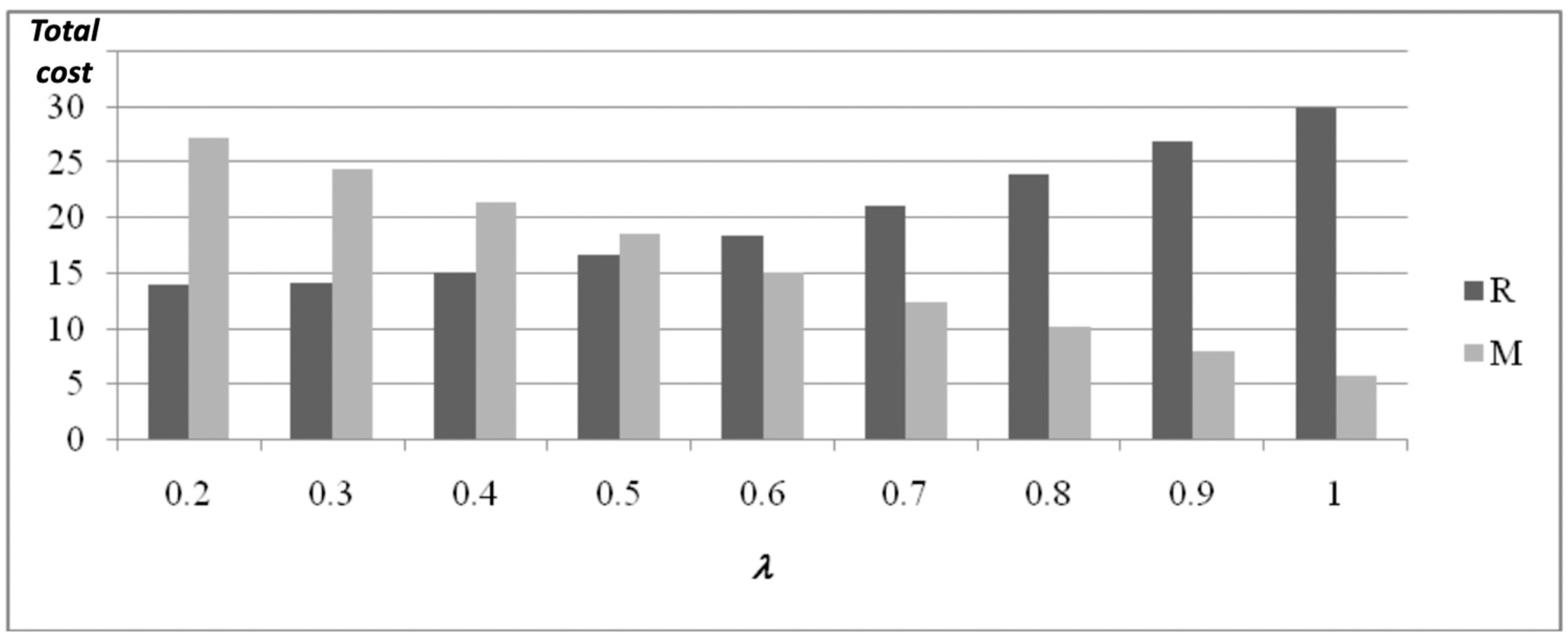
R (remanufacturing flow) represents the sum of cost components related inventory holding cost of Returned products inventory, Recoverable inventory, and Serviceable inventory filled by RL, as well as setup costs on SL and RL. M (manufacturing flow) represents the inventory holding cost of Serviceable inventory filled by ML, plus ML setup costs (see Figure 4).
In Figure 5, the two main flows’ cost components (R and M) are presented for different λ values (where λ1 = λ2 = λ3 = λ, without a loss of generality, as all parameter values have been made equal for the three items).
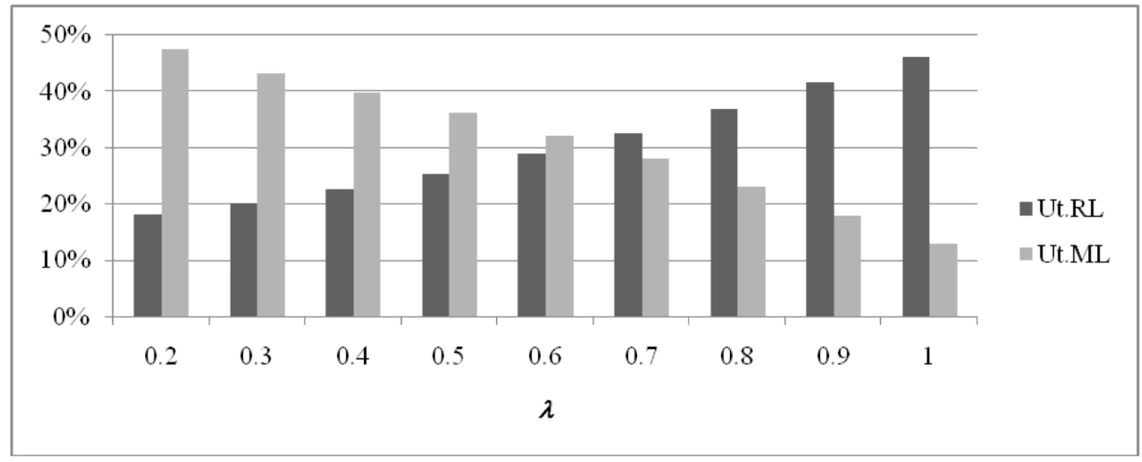
As shown in Figure 5, the cost related to the remanufacturing flow R increases for increasing values of λ, while for the behavior of the manufacturing flow M related cost the relationship is the opposite (it decreases for increasing values of λ). This is mainly due to the utilization of resources on the two flows. When the λ value is small, a few products are remanufactured, while almost all the demand is satisfied by new products, manufactured on ML. By increasing values of λ, the utilization of the remanufacturing flow increases, and also its related costs, while the cost associated with the manufacturing flow decreases, together with its utilization. This is presented in Figure 6.
The results suggest that there is a value λ*, which is the value of disposal rate that minimizes total system cost TC. When the amount of returns that have been deemed suitable for remanufacturing operations is greater than λi*βiDi, it is more convenient to dispose of the excess quantity and to pay for the production of new products.
In Figure 7, the different cost components solutions obtained for the minimum, best, and maximum values of λ are illustrated. Solutions presented as λ = 0.2 and λ = 1.0 seem to be not so balanced as the best solution found for λ* = 0.7, as presented in Figure 7.
In fact, starting from the setup costs, in the solution that involves λ* = 0.7 they are all equal on the three production lines, while they are not balanced in the solutions (the lowest and the highest value of λ, respectively). Looking at inventory holding cost (excluding Returned products and Recoverable inventories, whose holding costs are almost negligible in all presented solutions), the Serviceable inventory part filled by RL and ML is more balanced for λ* = 0.7 than for the other two proposed solutions. In order to confirm the balancing of costs, we must determine the best production frequencies (which allows for cost minimization) because it enables the determination of the best disposal rate to implement in the system, with the aim of minimizing TC.
Moreover, in order to understand how the production rate (or, as in this case, the remanufacturing rate) influences the total system cost, a sensitivity analysis on the production rate on RL is proposed.
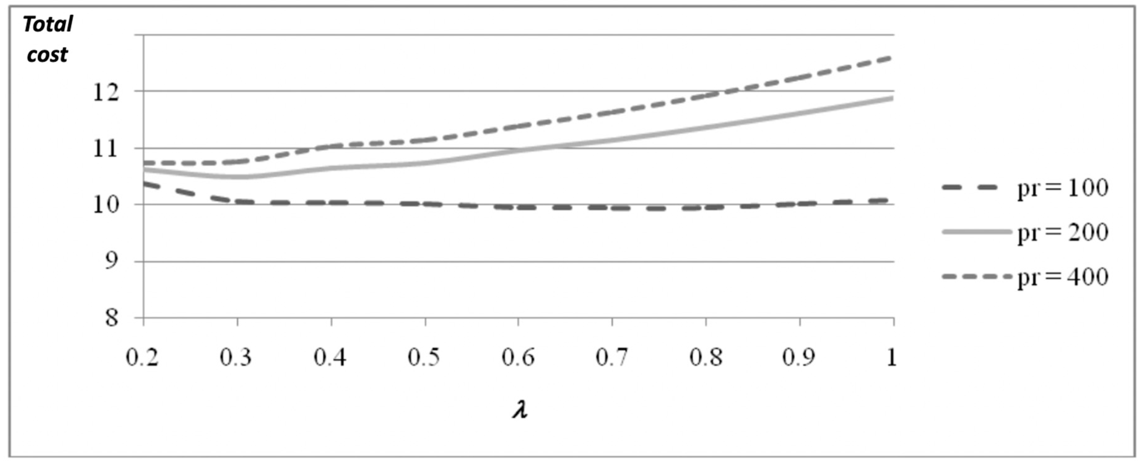
In Figure 8 the behavior of TC for different values of pr and λ is presented. For the case pr = 100, no feasible solutions have been found for values of λ greater than 0.7, due to the high values of RL utilization that can be detected.
For pr = 200 and pr = 400, such high values of RL utilization do not appear, and so the maximum value of λ that can be considered is 1 (100% of returned products are selected to be remanufactured). The value λ* = 0.7 has been found to be the best for the three considered cases, and the different cost components associated with such solutions are presented in Figure 9.
Once again, from Figure 9, Figure 10 and Figure 11, and considering that Figure 9 presents the best solution, related to λ* = 0.7, the better balancing of the two components of the Serviceable inventory holding cost (one related to the part filled by RL, and the other filled by ML), allows for a better solution, i.e., a smaller TC value. (In Figure 11 the case pr = 100 is absent, as this value does not generate feasible solutions for λ > 0.7). Utilization values for pr = 100 and 400 pr = 400 are illustrated in Figure 12 and Figure 13, respectively.
In all presented results and figures, TC and its components are considered for the discussion of the influence of λ and pr values, considering the sum of costs related to all items. The same conclusions on the effects of λ and pr are also valid for single items; the analysis presented in Appendix A is the proof.
5. Conclusions and Future Research
When sorting activities and manufacturing–remanufacturing operations are performed in a multi-item production system, adopting an optimized lot sizing policy determined by the best values of production frequencies on all production lines involved in the system could be very useful instead of implementing what is named the Common Cycle policy, which only allows the production of one lot of each item on each production line.
Using an adaptation of the data presented by [25] related to a real auto parts company, a model with three different production lines and a three-level inventory system has been developed.
For the specific case study, the optimal production frequencies of all items were determined for all production lines, on the basis of the balancing of setup and inventory holding costs related to the overall system and according to two fundamental feasibility conditions, i.e., the maximum allowed capacity utilization of resources (production lines) and the absence of production interference among lots of different items for each resource.
In this model, return rates and disposal percentage have been considered, and the effects of the disposal percentage λ has been studied on the utilization of the limited capacity of the resources involved in the system. The results show that there is always a best value of λ that minimizes the total cost of the manufacturing–remanufacturing system. Moreover, such results are valid for both a single-item system and a multi-item one, considering different remanufacturing rates; in fact, it has been found that in all performed numerical analyses, when increasing the disposal rate the utilization of RL increases, together with the costs associated with the so-called Remanufacturing flow (R) of the system, while the costs related to ML and Manufacturing flow decrease.
A possible direction for further studies could be represented by considering variable production rates on manufacturing and remanufacturing production lines, whose values will be assumed as decision variables of the model. The objective function that must be minimized is the system total cost; such an issue could also be related to the energy consumption reduction area (see [29,30,31,32]), which is involved in the energy efficiency management framework. Another possible research direction could be to consider the shortage cost component in total cost function for the different stocks present in the production line considered.
Funding
This research received no external funding.
Conflicts of Interest
The author declares no conflict of interest.
Appendix A
For the single-item case (Figure A1, Figure A2 and Figure A3), RL utilization increases for increasing values of λ, while ML utilization decreases. In this case, also for pr = 100, it is possible to obtain a feasible solution with λ > 0.7, thanks to the lower utilization of resources (single item).
Figure A1.
RL and ML utilization values for a single item (pr = 100).

Figure A2.
RL and ML utilization values for a single item (pr = 200).

Figure A3.
RL and ML utilization values for a single item (pr = 400).

For increasing values of pr (Figure A4), the optimal TC increases; for pr = 100, the best planned disposal rate involves a value of λ = 0.7, for pr = 200, the best value of λ is found at 0.3, and for pr = 400 the optimal TC is determined with λ = 0.2.
Figure A4.
Total cost for different values of pr and λ, for a single item.

For the case pr = 100, the best TC value has been found for λ = 0.7. As illustrated in Figure A5, when λ = 0.7, all the cost components are better balanced than in the other two solutions, where λ = 0.2 and λ = 1.0, respectively.
Figure A5.
Total cost components for different values of λ (pr = 100).

Look, for example, at the Serviceable inventory holding cost: the two light gray columns representing the Serviceable inventory filled by RL and ML are quite similar; in fact, looking at the black columns (corresponding to λ = 0.2), one can see that the Serviceable inventory filled by RL is much smaller than the other part, while for the dark gray columns associated with the solution where λ = 1.0, the situation is the opposite (more Serviceable inventory is filled by ML).
Also, the three setup cost components are better balanced for the solution with λ = 0.7; on the other hand, for λ = 0.2, ML-associated costs are higher than those related to RL, while for the solution associated with λ = 1.0 the situation is the opposite: higher cost components are related to RL.
References
- Teunter, R.H.; Vlachos, D. On the necessity of a disposal option for returned products that can be remanufactured. Int. J. Prod. Econ. 2002, 75, 257–266. [Google Scholar] [CrossRef]
- Dekker, R.; Fleischmann, M.; Inderfuth, K.; Van Wassenhove, L.N. Reverse Logistics: Quantitative Models for Closed Loop Supply Chains; Springer: Berlin/Heidelberg, Germany, 2004. [Google Scholar]
- Tang, O.; Teunter, R. Economic Lot Scheduling Problem with Returns. Prod. Oper. Manag. 2006, 15, 488–497. [Google Scholar] [CrossRef]
- Rogers, J. A Computational Approach to the Economic Lot Scheduling Problem. Manag. Sci. 1958, 4, 264–291. [Google Scholar] [CrossRef]
- Mabini, M.C.; Pintelon, L.M.; Gelders, L.F. EOQ type formulations for controlling repairable inventories. Int. J. Prod. Econ. 1992, 28, 21–33. [Google Scholar] [CrossRef]
- Schrady, D.A. A deterministic inventory model for repairable items. Nav. Res. Logist. Q. 1967, 14, 391–398. [Google Scholar] [CrossRef]
- Richter, K. The EOQ repair and waste disposal model with variable setup numbers. Eur. J. Oper. Res. 1996, 96, 313–324. [Google Scholar] [CrossRef]
- Richter, K. The extended EOQ repair and waste disposal model. Int. J. Prod. Econ. 1996, 45, 443–447. [Google Scholar] [CrossRef]
- Richter, K.; Dobos, I. Analysis of the EOQ repair and waste disposal problem with integer setup numbers. Int. J. Prod. Econ. 1999, 59, 463–467. [Google Scholar] [CrossRef]
- Dobos, I.; Richter, K. A production/recycling model with stationary demand and return rates. Cent. Eur. J. Oper. Res. 2003, 11, 35–46. [Google Scholar] [CrossRef]
- Dobos, I.; Richter, K. An extended production/recycling model with stationary demand and return rates. Int. J. Prod. Econ. 2004, 90, 311–323. [Google Scholar] [CrossRef]
- Teunter, R.H. Economic Ordering Quantities for Recoverable Item Inventory Systems. Nav. Res. Logist. 2001, 48, 484–495. [Google Scholar] [CrossRef]
- Teunter, R.H. Lot-sizing for inventory systems with product recovery. Comput. Ind. Eng. 2004, 46, 431–441. [Google Scholar] [CrossRef] [Green Version]
- Aras, N.; Verter, V.; Boyaci, T. Coordination and Priority Decisions in Hybrid Manufacturing/Remanufacturing Systems. Prod. Oper. Manag. 2006, 15, 528–543. [Google Scholar] [CrossRef]
- Yuan, K.; Gao, Y. Manufacturing and Remanufacturing Lot-size Model with Backordering and Disposal. In Proceedings of the 4th International Conference on Wireless Communications, Networking and Mobile Computing, WiCOM’08, Dalian, China, 12–17 October 2008. [Google Scholar]
- Galbreth, M.R.; Blackburn, J.D. Optimal Acquisition and Sorting Policies for Remanufacturing. Prod. Oper. Manag. 2009, 15, 384–392. [Google Scholar] [CrossRef]
- Schulz, T.; Ferretti, I. On the alignment of lot sizing decisions in a remanufacturing system in the presence of random yield. J. Remanuf. 2011, 1, 3. [Google Scholar] [CrossRef] [Green Version]
- Chang, Y.J.; Yao, M.J. New Heuristics for Solving the Economic Lot Scheduling Problem with Reworks. J. Ind. Manag. Optim. 2011, 7, 229–251. [Google Scholar] [CrossRef]
- El Saadany, A.M.A.; Jaber, M.Y. A production/remanufacturing inventory model with price and quality dependant return rate. Comput. Ind. Eng. 2010, 58, 352–362. [Google Scholar] [CrossRef]
- van der Laan, E.; Dekker, R.; Salomon, M. Product remanufacturing and disposal: A numerical comparison of alternative control strategies. Int. J. Prod. Econ. 1996, 45, 489–498. [Google Scholar] [CrossRef] [Green Version]
- van der Laan, E.; Salomon, M. Production planning and inventory control with remanufacturing and disposal. Eur. J. Oper. Res. 1997, 102, 264–278. [Google Scholar] [CrossRef] [Green Version]
- Zanoni, S.; Segerstedt, A.; Tang, O.; Mazzoldi, L. Multi-product economic lot scheduling problem with manufacturing and remanufacturing using a basic period policy. Comput. Ind. Eng. 2012, 62, 1025–1033. [Google Scholar] [CrossRef] [Green Version]
- Segerstedt, A. Lot sizes in a capacity constrained facility with available initial inventories. Int. J. Prod. Econ. 1999, 59, 469–475. [Google Scholar] [CrossRef]
- Berut, O.; Tasgetiren, M.F. A discrete artificial bee colony algorithm for the Economic Lot Scheduling problem with returns. In Proceedings of the 2014 IEEE Congress on Evolutionary Computation, CEC 2014, Beijing, China, 6–11 July 2014. [Google Scholar]
- Teunter, R.; Kaparis, K.; Tang, O. Multi-product economic lot scheduling problem with separate production lines for manufacturing and remanufacturing. Eur. J. Oper. Res. 2008, 191, 1241–1253. [Google Scholar] [CrossRef] [Green Version]
- Teunter, R.; Tang, O.; Kaparis, K. Heuristics for the economic lot scheduling problem with returns. Int. J. Prod. Econ. 2009, 118, 323–330. [Google Scholar] [CrossRef] [Green Version]
- Konstantaras, I.; Skouri, K.; Jaber, M.Y. Lot sizing for a recoverable product with inspection and sorting. Comput. Ind. Eng. 2010, 58, 452–462. [Google Scholar] [CrossRef]
- Teunter, R.H.; van der Laan Eand Inderfurth, K. How to set the holding cost rates in average cost inventory models with reverse logistics. Omega 2000, 28, 409–415. [Google Scholar] [CrossRef]
- Gutowski, T.G.; Branham, M.S.; Dahmus, J.B.; Jones, A.J.; Thiriez, A.; Sekulic, D.P. Thermodynamic Analysis of Resources Used in Manufacturing Processes. Environ. Sci. Technol. 2009, 43, 1584–1590. [Google Scholar] [CrossRef] [PubMed]
- Zanoni, S.; Ferretti, I.; Zavanella, L.E. Energy Value Stream methods with auxiliary systems. In Proceedings of the Eceee Industrial Summer Study Proceedings, Berlin, Germany, 11–13 June 2018; pp. 281–291. [Google Scholar]
- Zavanella, L.E.; Zanoni, S.; Ferretti, I.; Mazzoldi, L. Energy demand in production systems: A queuing theory perspective. Int. J. Prod. Econ. 2015, 170, 393–400. [Google Scholar] [CrossRef]
- Zavanella, L.E.; Ferretti, I.; Zanoni, S.; Bettoni, L. A queuing approach for energy supply in manufacturing facilities. IFIP Adv. Inf. Commun. Technol. 2013, 459, 670–679. [Google Scholar]
Figure 1.
The manufacturing–remanufacturing system with sorting.

Figure 2.
Production lines’ activation scheduling.

Figure 3.
The serviceable inventory related to ML action.

Figure 4.
The system main flows.

Figure 5.
Main flows cost components (pri = 200, ∀i).

Figure 6.
RL and ML utilization values (pri = 200, ∀i).

Figure 7.
Total cost components (pri = 200, ∀i).

Figure 8.
Total cost for different values of pr and λ.

Figure 9.
Total cost components for different values of pr (λ* = 0.7).

Figure 10.
Total cost components for different values of pr (λ = 0.2).

Figure 11.
Total cost components for different values of pr (λ = 1.0).

Figure 12.
RL and ML utilization values (pr = 100).

Figure 13.
RL and ML utilization values (pr = 400).


Table 1.
The existing literature on the addressed model features.
| Manufacturing Option | Remanufacturing Option | EOQ Approach | Basic Period Approach | Common Cycle Approach | Sorting Line and Disposal Option | |
|---|---|---|---|---|---|---|
| Teunter et al. 2008 | x | x | x | |||
| Konstantaras et al. 2010 | x | x | x | |||
| Zanoni et al. 2012 | x | x | x | |||
| This work | x | x | x | x |
Table 2.
Cost components.
| Costs | Equation |
|---|---|
| Setup Costs of SL | Equation (14) |
| Setup Costs of RL | Equation (19) |
| Setup Costs of ML | Equation (20) |
| Inventory Holding Costs of Returned Products Inventory | Equation (13) |
| Inventory Holding Costs of Recoverable Inventory λipsi = pri | Equation (15) |
| Inventory Holding Costs of Recoverable Inventory λipsi > pri | Equation (16) |
| Inventory Holding Costs of Recoverable Inventory λpsi < pri | Equation (17) |
| Inventory Holding Costs of Serviceable Inventory | Equation (18) |
Table 3.
Numerical analysis: data (N = 3).
| Item 1 | Item 2 | Item 3 | |
|---|---|---|---|
| Di | 50 | 50 | 50 |
| pmi | 400 | 400 | 400 |
| pri | 200 | 200 | 200 |
| psi | 500 | 500 | 500 |
| hsi | 0.02 | 0.02 | 0.02 |
| hri | 0.014 | 0.014 | 0.014 |
| hui | 0.0098 | 0.0098 | 0.0098 |
| Ai | 50 | 50 | 50 |
| si | 1 | 1 | 1 |
| βi | 0.8 | 0.8 | 0.8 |
© 2020 by the author. Licensee MDPI, Basel, Switzerland. This article is an open access article distributed under the terms and conditions of the Creative Commons Attribution (CC BY) license (http://creativecommons.org/licenses/by/4.0/).
Share and Cite
MDPI and ACS Style
Ferretti, I. Multiproduct Economic Lot Scheduling Problem with Returns and Sorting Line. Systems 2020, 8, 16. https://0-doi-org.brum.beds.ac.uk/10.3390/systems8020016
AMA Style
Ferretti I. Multiproduct Economic Lot Scheduling Problem with Returns and Sorting Line. Systems. 2020; 8(2):16. https://0-doi-org.brum.beds.ac.uk/10.3390/systems8020016
Chicago/Turabian StyleFerretti, Ivan. 2020. "Multiproduct Economic Lot Scheduling Problem with Returns and Sorting Line" Systems 8, no. 2: 16. https://0-doi-org.brum.beds.ac.uk/10.3390/systems8020016
Note that from the first issue of 2016, this journal uses article numbers instead of page numbers. See further details here.