
CFD Simulation of an Internally Cooled Biomass Fixed-Bed Combustion Plant


Grupo de Tecnología Energética (GTE), CINTECX, Universidade de Vigo, 36310 Vigo, Spain
*
Author to whom correspondence should be addressed.
Resources 2021, 10(8), 77; https://0-doi-org.brum.beds.ac.uk/10.3390/resources10080077
Submission received: 18 June 2021
/
Revised: 14 July 2021
/
Accepted: 20 July 2021
/
Published: 23 July 2021
(This article belongs to the Special Issue Waste-to-Energy Systems in Standalone, Integrated and Hybrid Configurations)
Abstract
:The reduction of bed temperature in fixed-bed biomass combustion is an effective measure to lower pollutant emissions. Air staging and bed cooling solutions are active strategies to decrease the fuel bed temperature. This work presents a CFD study of a biomass fixed-bed combustion plant that is equipped with an internal cooling bed system. Eight different cases are calculated to analyze the effect of the total airflow, air staging ratios and bed cooling system on biomass combustion. The findings are validated against experimental data from the literature. The results show good accordance between the numerical results and the experimental data. The primary airflow rate has the biggest influence on the bed’s maximum temperatures. The internal bed cooling system is able to achieve an average bed temperature reduction of 21%, slowing the biomass thermal conversion processes. Bed cooling techniques can be combined with air staging and primary airflow reduction to reduce bed temperatures in order to reduce pollutant emissions and other undesirable phenomena, such as fouling or slagging.
1. Introduction
Biomass has been the main source of energy for heating and cooking since ancient times, due to its diversity, worldwide availability and usability [1,2]. Over the last few decades, interest in biomass as an alternative energy source to fossil fuels has grown significantly. From a sustainability point of view, the combustion of solid biomass to convert into heat and power has attracted great interest, since it allows industries to obtain energy from wastes in an energy-efficient way [2].
However, the combustion of solid biomass has some associated problems that in some cases can hinder the transition to this energy source. For example, although the combustion of biomass can be considered neutral regarding carbon dioxide emissions, other pollutants harmful to human health, such as particulate matter (PM) or NOx, are present [3,4].
In addition, the presence of alkali metals and other inorganic compounds in the biomass composition can cause ash-related problems and corrosion in biomass combustion systems. Higher content of alkalis, such as sodium and potassium, reduces the melting point of the ash. The condensation of these inorganic vapors on the heat exchange surfaces is the starting point for the generation of a fouling layer. The reduction of the ash fusion temperature also encourages the formation of slag on the surfaces in contact with the fuel bed. The fouling and slagging cause a decrease in thermal efficiency of the combustion systems, and may cause system damage [5,6,7,8,9].
To reduce these problems, several techniques can be utilized. Differentiation can be made between primary measures, if they directly affect the combustion process while trying to avoid these phenomena, and secondary measures, such as the treatment and filtering of exhaust gases or the removal of fouling and slagging.
The most popular primary measures are focused on controlling the air injection and the temperature of the solid fuel bed. Different studies have shown how air staging reduces PM and gaseous emissions [10,11,12]. Low primary air ratios lead to a reduction in PM emissions, as the lower air velocity in the bed results in less elutriation [10,12]. In addition, staged combustion with secondary, and even tertiary, air injections help to achieve an efficient flue gas burnout and can reduce NOx emissions [11,12]. Using low air excess ratios for the primary air also helps to reduce the temperatures of the solid fuel bed, lowering the risk of fouling and slagging due to ash melting [12]. Flue gas recirculation and bed cooling techniques can also be used to reduce the temperatures of the bed. Flue gas recirculation (FGR) consists of replacing a portion of the primary air with flue gas that has previously been cooled, to reduce the oxygen concentration and, thus, reducing the temperature of the fuel bed and slowing its thermal conversion process. Studies have shown how FGR helps to reduce the unburnt species, PM and NOx emissions, and the slagging in the bed [12,13,14,15]. Bed cooling solutions consist of the refrigeration of the solid fuel bed. In medium- and large-scale systems, water-cooled grates are used to refrigerate the bed. There are studies on the implementation of cooling systems formed by a water pipe surrounding the fuel bed in domestic biomass boilers, showing a reduction of PM emissions without affecting other combustion parameters [16,17].
In this context, Pérez-Orozco et al. presented an experimental small-scale biomass combustion system designed to test the influence of air staging, FGR and bed cooling on biomass combustion emissions [18]. The most novel part of this plant is the complete refrigeration system that also includes the fuel bed. To allow the characterization of the temperature distribution inside the combustion system and the pollutant emissions, the plant is equipped with thermocouples located in different zones, as well as a gas analyzer and a low-pressure impactor connected to the exhaust. Several experimental studies have already been carried out, testing the stability and repeatability of the facility, and analyzing the effectiveness of using different air ratios, FGR and bed cooling for reducing pollutant emissions [13,14,18,19].
Computational Fluid Dynamics (CFD) software is a useful tool for studying biomass combustion and analyzing combustion systems. Numerical tools allow the addressing of aspects that are not easy to characterize experimentally and reducing the costs of the design and optimization of biomass combustion systems.
CFD codes can solve fluid flow and heat transfer processes, as well as homogeneous chemical reactions occurring in the gas phase. However, to simulate the solid biomass thermal conversion process, it is necessary to use sub-models. One-dimensional sub-models, based on empirical correlations or on biomass thermal conversion models, can be easily coupled with the CFD being a simple option with a low computational cost [20,21,22]. Numerical studies using coupled empirical one-dimensional bed models have shown that enhanced air staging allows a significant reduction of particulate matter and nitrogen oxide emissions [21,22]. However, these models cannot predict the state of the solid fuel bed. In order to track each fuel particle individually and characterize its thermal conversion process, it is necessary to employ Lagrangian models, such as the discrete element method (DEM) or the discrete phase model (DPM), coupled with biomass thermal conversion models [23,24]. These models allow a more realistic characterization of the solid fuel bed but have a high computational cost.
Eulerian models have a lower computational cost than Lagrangian models, being a more comprehensive approach than one-dimensional models [23]. These models usually consider two zones, the bed, defined as a porous zone where the solid and gas phases coexist, and the freeboard, set as a simple fluid, allowing dynamic coupling between both phases [25,26,27,28,29]. Eulerian models have been successfully used to simulate systems under different air/oxy-fuel conditions [28] and on different scales, from small experimental plants [27], to medium- [25] and large-scale systems [26,29]. Although these models do not treat the fuel bed as individual particles, physics algorithms can be implemented to simulate the movements and compaction of the solid fuel inside the systems [30,31]. In this work, the Eulerian biomass thermal conversion model (EBiTCoM), developed by the Energy Technology Group (GTE) of the University of Vigo, will be used.
The EBiTCoM is fully integrated into the CFD commercial code ANSYS-Fluent as a user-defined function (UDF) programmed in C/C++ [32]. The model allows the simulation of fixed-bed biomass thermal conversion systems. The model has been used to simulate various systems, from small lab-scale devices to industrial-scale systems, such as gasifiers and boilers [26,30,33,34,35,36,37].
This work extends and complements the work of Pérez-Orozco et al. by presenting a CFD study on the influence of bed cooling and air staging on biomass combustion. The experimental small-scale biomass combustion system presented by Pérez -Orozco et al. will be simulated, validating the numerical modeling against the experimental data, allowing us to study the influence of bed cooling on the combustion [19]. For this purpose, several CFD cases for different primary airflows and staging ratios, and with the bed cooling system enabled or disabled, will be studied. To validate the results, the temperature profiles inside the solid fuel bed and along the combustion unit measured in the experimental tests will be compared with the simulation results. The CFD results will be used to analyze the effect of air staging and bed cooling on different parameters, such as the fuel conversion ratio, bed morphology, temperatures, gaseous emissions, etc.
2. Model
In this work, the commercial CFD code ANSYS-Fluent 2020 R1 will be used. This software can solve the characterization of fluid phases, including the heat transfer phenomena and the homogeneous gas reactions. The EBiTCoM, which is embedded in the CFD code as a UDF, will characterize the solid fuel bed and its thermal conversion, allowing the dynamic coupling between the bed and the gas phase.
The main features, assumptions and approaches of the model are presented below. A more detailed description of the EBiTCoM characteristics and procedures can be found in previously published works [26,30,35,36].
2.1. Solid Phase
The bed is modeled as a porous zone where the solid fuel and the gas phase coexist. In this zone, user-defined scalars (UDS) are used to characterize the solid fuel properties in each cell. The scalars, which represent local volume-averaged values for each cell, are: solid fraction (m3solid/m3cell), solid temperature (K), moisture density (kg/m3solid), dry wood density (kg/m3solid), char density (kg/m3solid), ash density (kg/m3solid) and third power of the particle average diameter (m3).
The solid fraction scalar defines the ratio of cell volume that is occupied by solid fuel. The maximum value of this variable is limited to the maximum packing factor of the fuel. The densities define the composition of that solid volume. Although this approach does not consider each individual fuel particle, the particle average diameter characterizes the size of the theoretical particle (or particles) that is represented by the solid volume of each cell (Eulerian approach). The temperature of the solid volume in each cell is considered homogeneous, since the EBiTCoM is based on a thermally thin assumption and is controlled by the solid temperature scalar.
The transient evolution of each UDS is controlled by a transport equation (Table 1). The terms on the right-hand side represent the consumption and generation of each variable. The shrinkage of the solid, which is reflected in the solid fraction and the particle diameter, only occurs during wood devolatilization and char generation [36]. In the transport equation of the solid temperature scalar (Equation (1) there is a diffusive term, which represents the equivalent thermal conductivity between the solids. The diffusive term is not present in the other equations because there is no mass diffusion between the solids. The ash is non-reactive, but it can be compacted when the solid fuel bed collapses, due to the shrinkage of the particles [30].
Apart from the shrinkage and compaction, the model also includes physics algorithms to simulate the effect of gravity on the solid fuel bed, which, being a granular material, will have a tendency to form piles [31,38]. In addition, the model has different fuel feeding methods, to simulate the feeding mechanisms of different combustion systems. In this case, a feeding method that uses the ANSYS-Fluent discrete phase model (DPM) will be used. This method tracks the trajectories of the fuel particles falling from the fuel inlet to the bed zone, and deploys the corresponding fresh fuel mass in the final particle position [36].
In Table 2, the equations defining the consumption rates of the solid fuel components are shown. The moisture of the solid fuel starts to evaporate when the temperature of the solid is equal to or higher than 373.15 K (Equation (8)). The particles dry from the outside inward. This means that when the outer layers of the particles are dry, there is still moisture on the inside. Because of this, the average temperature of the particle keeps rising before it is totally dried. To model this effect, half of the heat received by the solid is employed in the drying process, and the other half is in the heating of the solid fuel. The pyrolysis is modeled as three conversion processes, converting the dry wood into gas tar and char. The wood consumption ratio is the sum of the three Arrhenius equations that control these processes (Equation (9)). The char generated in the pyrolysis is consumed by direct oxidation and two gasification reactions, which are also controlled by Arrhenius equations. The char consumption ratio is the sum of the three reaction ratios, taking into account the diffusion of oxygen, carbon dioxide and water vapor for each respective reaction (Equation (10)).
The kinetics of the solid heterogeneous reactions are collected in Table 3 [39,40,41]. The ratio for CO/CO2 produced by the char oxidation (φ) is calculated by a temperature-dependent correlation [40,42].
The solid fuel exchanges energy with the gas phase by convection and radiation. The convective heat transfer coefficient is calculated by an experimental correlation to obtain the Nusselt number for particle-to-fluid heat transfer in packed beds [43]. In the same way, the mass transfer coefficients are calculated with an experimental correlation to obtain the Sherwood number [44]. The radiation heat exchange is calculated by a modified version of the discrete ordinates model to take into account the influence of the solid phase on the absorption and scattering coefficients of the cell and adding an emissivity term for the solid [30,45]. These heat exchanges between phases are computed using energy sources that absorb from or give energy to one of the phases and do the opposite in the other phase. Energy sources are also used to model the heat exchanges produced during the drying, devolatilization and char reactions.
2.2. Gas Phase
CFD codes have been extensively used to simulate biomass combustion in many types of systems. This software can solve the conservation equations applied to the gas phase with its built-in algorithms. In this case, the continuity, momentum, energy, turbulence, chemical species, and soot conservation equations are calculated.
The turbulence model used is the realizable k-ε model, which is commonly used in biomass combustion system simulations [23,25,26]. The radiation model chosen is the discrete ordinates model, which has been modified to take into account the contribution of the solid phase [45]. The finite rate–eddy dissipation (FR-ED) model, which is suitable for most biomass combustion cases since the turbulent mixing is the rate-limiting step in the consumption of the gaseous species, is used to compute the interaction of turbulence and kinetics [46]. The Moss-Brookes model is used for soot nucleation and reaction. The effect of the porous bed on the gas flow is modeled using a dispersed porous media approach with physical velocity condition and a momentum source [30].
During the thermal processes that affect the solid fuel, a series of gaseous emissions are released. The drying produces water vapor, and the heterogeneous char reactions produce CO, CO2 and H2, consuming O2, CO2 and H2O(v), respectively. To model the devolatilization, a simplified list of species is used. This includes CH4, C6H6, CO, CO2, H2 and H2O(v). The methane and benzene represent the light hydrocarbons and tars, respectively. The composition of the emissions is estimated by a method based on an elemental and energy balance equation system that is closed with two experimental expressions [47]. In this case, experimental CO and CH4 yields in the function of the temperature of pyrolysis are taken as the closure equations [48]. All the species generated and consumed in the solid fuel thermal processes are exchanged with the gas phase, using mass sources.
3. Methodology
In this work, the influence of bed cooling and air staging on biomass combustion will be studied. The biomass combustion pilot plant, presented by Pérez-Orozco et al. [18], will be simulated using CFD techniques. Several cases with different operating conditions will be calculated, and the results validated against experimental data. The CFD results will be used to analyze the influence of the solid fuel bed internal cooling and air staging on the biomass thermal conversion processes.
3.1. Experimental Plant
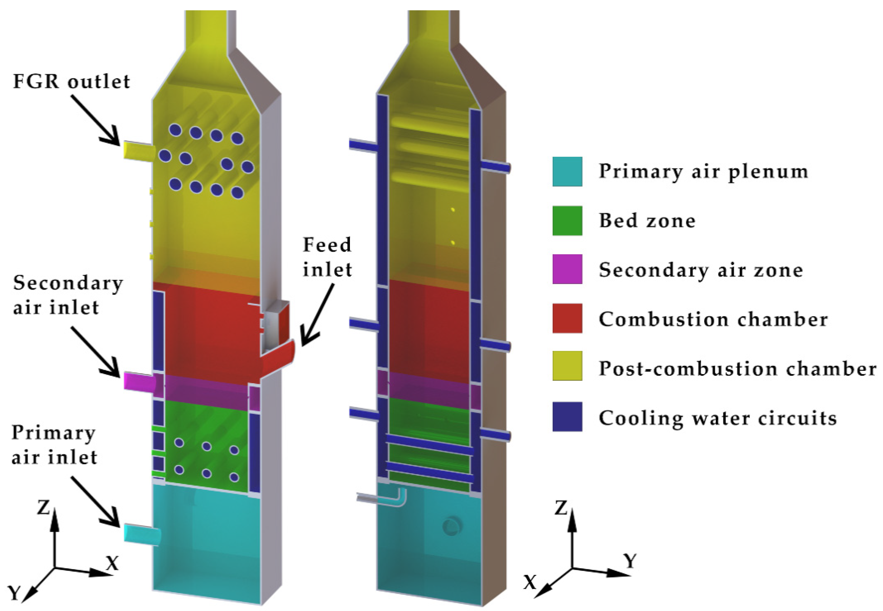
The system is an 11–18 kW overfed fixed-bed burner with a modular configuration and is designed to study different strategies for improving combustion [18,19]. The unit is made of stainless steel and divided into parts, within which the positions can be interchanged (Figure 1). From bottom to top, the first zone is the primary air plenum. The primary air enters the bed zone from the plenum through a grate with an internal cross-section of 150 × 150 mm and 625 holes of 3 mm diameter. The walls of the bed zone are water-cooled, and there are two rows of three tubes at 25 mm and 75 mm above the grate. These six tubes pass through the fuel bed, allowing for internal cooling. The secondary air module is located above the fuel bed. It has a single row of 45° oriented holes, to cause a swirling effect in the airflow. The next module is the combustion chamber, which has three cooled walls and one removable wall, where the fuel inlet is located. The last module is the post-combustion chamber and the chimney. This module has two refrigerated walls and three rows of four tubes acting as heat exchangers. In this zone, there is also the FGR outlet. However, for the cases studied in this work, this system will not be active.
The plant is equipped with different monitoring systems that allow us to measure variables such as air and water flow, temperatures, or emissions. Two centrifugal single inlet fans supply both primary and secondary airflows. The flows are measured using two hot-film air-mass sensors located at the inlets, regulated through throttle valves to change the air staging conditions. In addition, two flowmeters are used to measure the water flows of the bed cooling system and the combustion chamber cooling circuit.
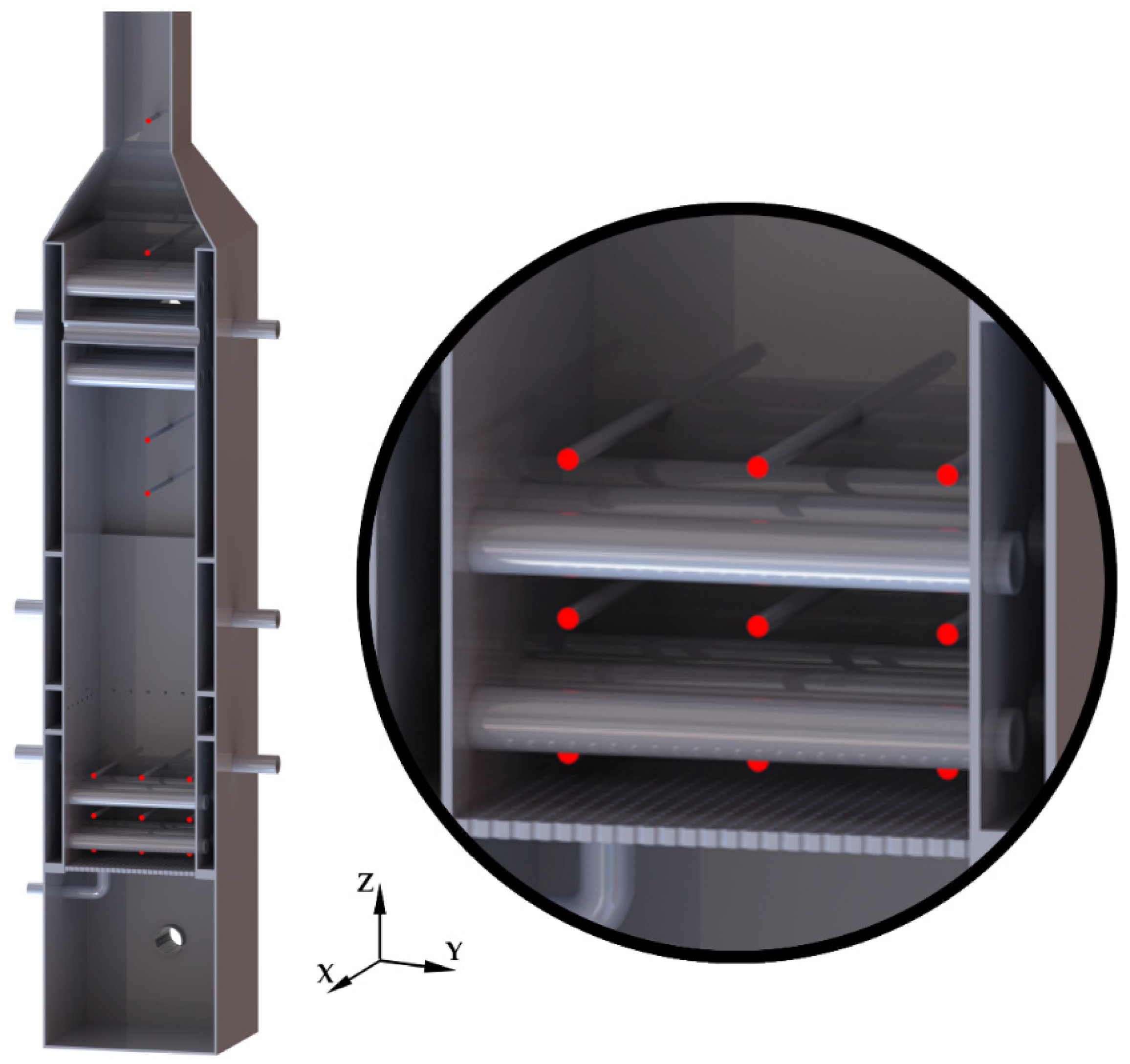
To measure the temperatures of the cooling water and inside the system, thermometers and thermocouples are used, respectively. The thermometers are placed at the inlets and outlets of the cooling circuits. Thermocouples of different types, depending on the expected temperatures in each area, are used to measure the temperatures along the combustion unit. In the bed module, there is a temperature mapping system consisting of three rows of three thermocouples, each located at three different heights. In the upper modules, there are several ports in the walls for the insertion of thermocouples. Figure 2 shows the thermocouple configuration, used in the experimental tests, that was taken as a reference for this work [19].
The bed temperatures were measured at three heights (12 mm, 50 mm, and 95 mm above the grate). The first row of thermocouples is located between the grate and the lower tubes of the bed cooling system, the second row between the two rows of tubes, and the third one above the upper tubes. The temperatures measured by the three thermocouples at each height are averaged into one temperature to provide more homogeneous information. The other thermocouples are located at 410, 470, 645, and 835 mm above the grate, with their tips at the central z-axis.
3.2. Fuel and Operating Conditions
The fuel used in the experimental runs was commercial wood pellets with an average size of 6 mm in diameter and 20 mm in length. The fuel proximate and ultimate analyses results, and the heating values, are given in Table 5 [19]. The fuel data will be used to establish the properties of the fresh fuel and to obtain the composition of the pyrolysis volatile.
To assess the effect of the total airflow, the staging level and the cooled bed on the combustion, eight different experimental tests were carried out by Pérez-Orozco et al. [19]. These eight tests result from the combination of two total airflows, two staging ratios, and the activation of the bed cooling system.
In Table 6, the list of experimental tests that are going to be simulated is presented. As in the experimental work, the name used to identify each case will be the primary airflow value, followed by CB or raw if the bed cooling system is activated or not, respectively.
3.3. Discretization and Boundary Conditions
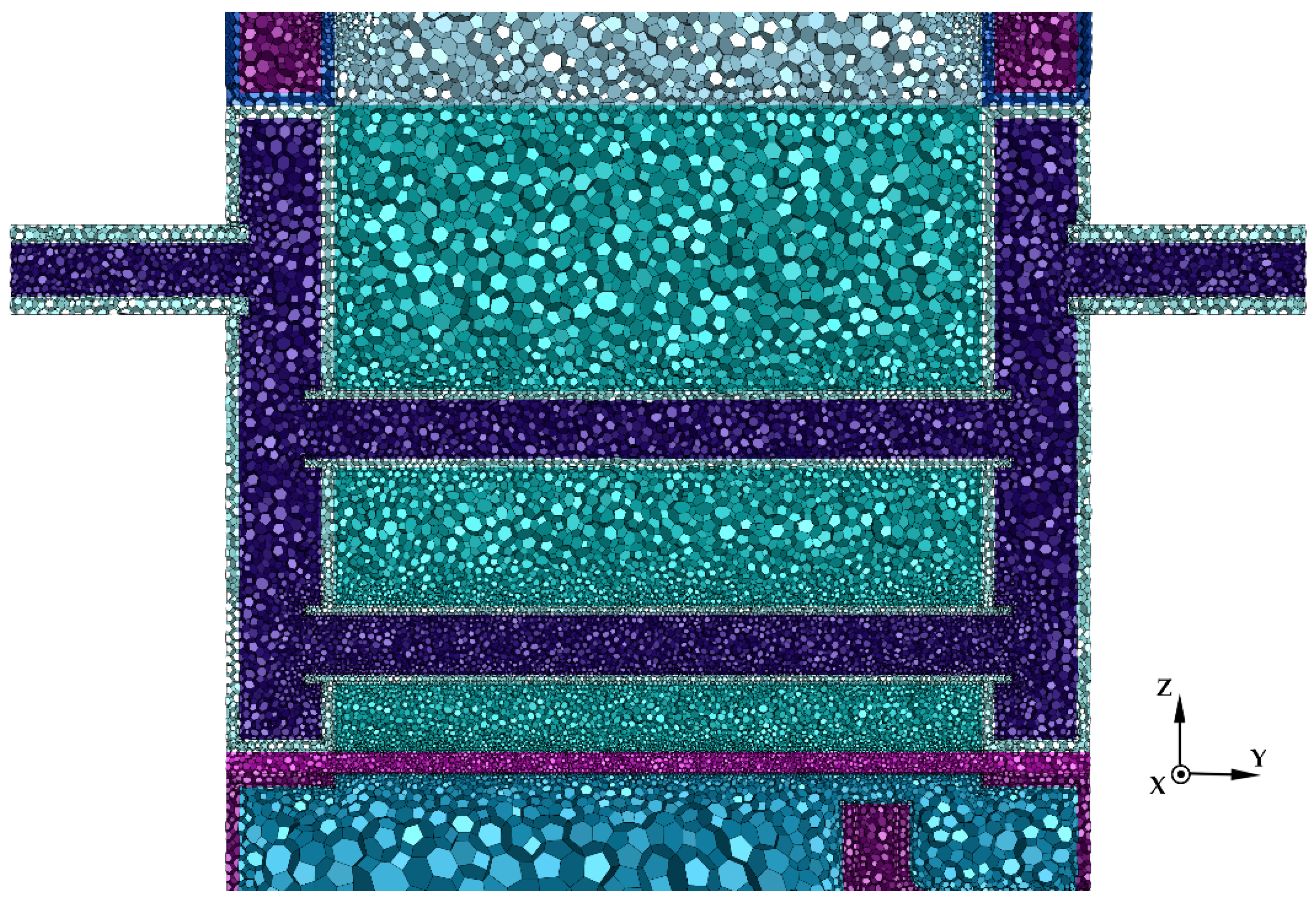
To discretize the domain, a polyhedral mesh is chosen, in order to reduce the number of elements needed, compared with a tetrahedral mesh. In addition, this type of mesh has already been used in biomass combustion simulations using the EBiTCoM model and has shown a better response in the bed physics algorithms, compared with other morphologies [26,31,38]. The domain includes the interior of the combustion plant, the solid walls, and the water-cooling circuits.
The mesh is more refined near the walls and where higher gradients are expected, as in the bed region near the grate, or in the secondary air injection zone. To reduce the total number of elements needed, a growth ratio was applied to the three-dimensional cells from the walls toward the center of the volumes, as seen in Figure 3. After carrying out a mesh independence study, a final mesh of more than 3 million polyhedral cells was chosen.
All the walls are made of steel, and its thermal properties are applied to them. Convective heat transfer in still air conditions is applied to the external walls. An emissivity value of 0.8 is applied to the internal walls, to assess the effect of the fouling layer over the walls [26].
The primary and secondary air airflows for each case are given in Table 6. The combustion and post-combustion chambers’ cooling systems are each supplied with 0.432 m3/h of water, and the bed cooling system, when active, with 0.576 m3/h of water at an average temperature of 52 °C.
The temperatures are monitored by an UDF function. This algorithm receives the coordinates of the thermocouples and searches the cell with the closest centroid to each coordinate. The temperature measured by each thermocouple is calculated as a function of the gas temperature at each cell and the incident radiation.
4. Results
A transient simulation is calculated for each case. Different variables are monitored to check if the combustion plant has reached its pseudo-steady state, as solid biomass combustion usually presents an oscillatory behavior. In addition, the pseudo-random fuel feeding method used in this work causes disturbances. Because of this, the monitored variables do not tend to stabilize to a constant value but instead describe periodic oscillations around it. When these oscillations are stable inside a constant range, it is considered that a pseudo-steady state has been reached. At this moment, the temperatures at the thermocouples are registered for 500 s of flowtime to obtain averaged values.
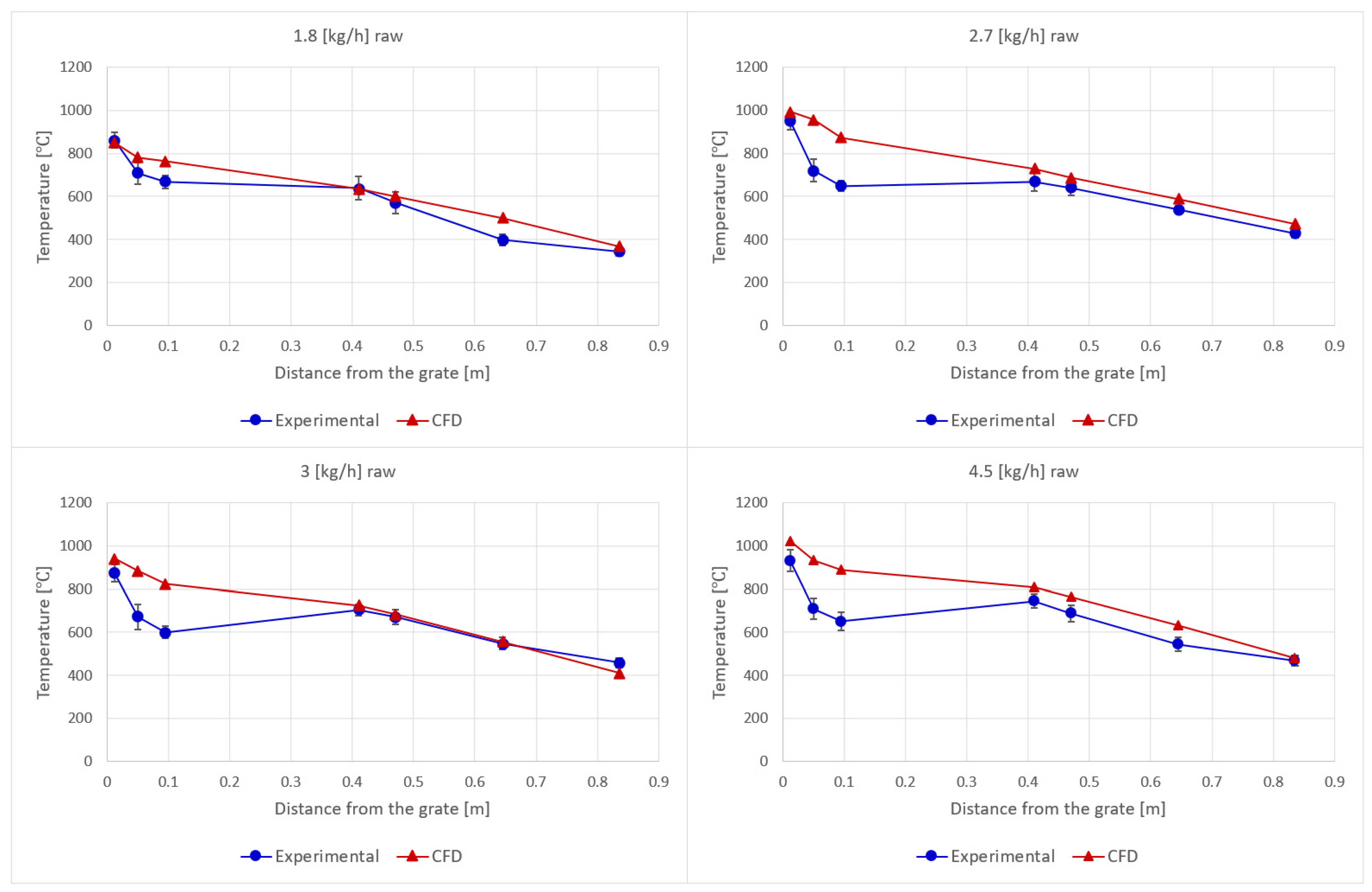
The simulation results are compared against the experimental measures presented by Pérez-Orozco et al. [19]. The temperature profiles represent the temperature variation along the central z-axis from the grate to the chimney of the combustion plant.
Figure 4 shows the comparisons of the experimental and numerical raw tests. It can be seen that the maximum temperatures, which are registered at the thermocouples located closest to the grate, are directly proportional to the primary airflows, increasing as the primary airflow rate increases. The maximum temperature is accurately predicted, with an average error of 6%. This deviation comes from a slight overestimation of the maximum temperature, which is higher in the cases with higher primary airflow. The middle and top row bed thermocouples’ experimental measurements show a temperature decrease that is not fully reflected in the CFD simulations. On average, the calculated bed temperatures are 21% higher than the measurements. This may be caused by the boundary conditions that are applied to the CFD case in the bed zone when the cooling bed circuit is off, which resulted in a more adiabatic situation than in the experimental tests. Another possible cause of this temperature overestimation in the bed zone might be the assumption that it is thermally thin. The consideration that the temperature of the solid in each cell is homogeneous throughout its volume causes faster heating rates [26]. This leads to faster drying and pyrolysis rates, reducing the layer of wood in the bed and increasing the proportion of char in it. A higher volume of char and a thinner wet wood layer results in a higher average bed temperature.
For the gas phase measurements, the predicted values show very good accordance, especially for the 6 kg/h total airflow cases (1.8 kg/h raw and 3 kg/h raw). For the 9 kg/h total airflow cases (2.7 kg/h raw and 4.5 kg/h raw), the numerical gas temperatures are 10% higher on average. For the four raw cases, the numerical gas temperatures have an average error of 8%.
In Figure 5, the obtained numerical results for the cooled bed tests are compared against the experimental data. In the four cases, the bed model predicts higher maximum temperatures, especially for the 9 kg/h total airflow cases (2.7 kg/h CB and 4.5 kg/h CB). For these two cases, 35% and 42% higher maximum temperatures are predicted, while for the 6 kg/h total airflow cases (1.8 kg/h CB and 3 kg/h CB), the maximum numerical temperatures registered are around 12% and 18% higher. In the same way as for the raw simulations, the temperature overestimation in the solid fuel bed is probably a result of the thermally thin assumption. Another possible cause of the temperature difference could be that if experimental tests take too long, or if there is poor cleaning between tests, an excessive accumulation of non-reactive ash at the surface of the grate may occur. The thickness of the ash layer can affect the temperature measurements of the lower thermocouples, decreasing the average temperature readings of the zone.
The influence of the bed cooling system in the temperature profiles of the solid fuel bed is clearly seen in all cases, both for CFD and experimental tests. The 9 kg/h total airflow cases show a higher temperature decrease than the 6 kg/h cases, which can be attributed to a higher temperature gradient, due to higher maximum temperatures. On average, for the four cases, at the higher row of bed thermocouples, the numerical temperatures are 30% higher than the experimental measures.
For the gas phase measures, the difference between CFD and experimental is smaller, especially for the 6 kg/h total airflow cases in which the temperature profiles show almost no deviation. For the 9 kg/h total airflow cases, the predicted temperatures are around 12% higher on average than the experimental ones. It can also be seen that in all cases, the temperature at the outlet is predicted with high accuracy.
Based on these results, it can be said that, although the model has shown a tendency to predict higher maximum bed temperatures than experimental ones, the error is within an acceptable range, and that the influence of the internal bed cooling system has been correctly modeled. Outside the bed region, in the freeboard, the numerical temperature profiles have shown great accuracy when compared with the experimental test results.
Once the CFD results have been validated, the influence of the different operating parameters on the combustion can be analyzed.
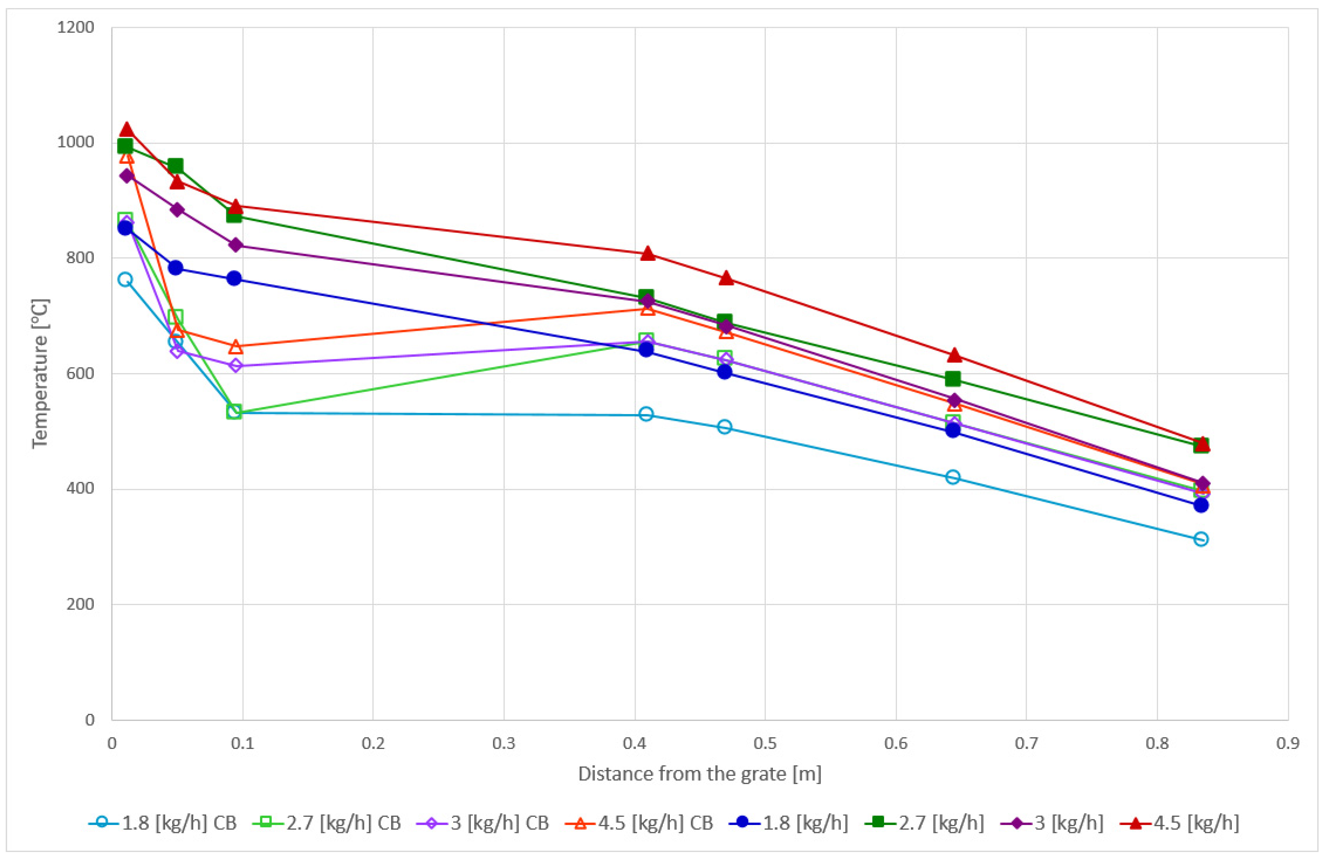
In Figure 6, the temperature profiles of the eight numerical studied cases can be seen. The primary airflow has a direct relationship with both maximum and average bed temperatures. Higher primary airflows lead to higher conversion ratios of the solid fuel, resulting in higher temperatures. In a similar way, increasing the total airflow also increases the average gas temperature along the length of the plant, which is directly related to the secondary airflow increase.
The bed cooling system allows an effective reduction of temperatures, both in the bed and along the length of the plant. Its effect is higher in the middle and upper part of the bed, where an average temperature decrease of 240 °C is achieved. In the bottom zone, closer to the grate, the temperature reduction achieved is around 87 °C. Outside the bed region, the effect of bed cooling is translated into an average temperature decrease of 73 °C. This accounts for an average reduction of 21% in bed temperatures and 12% in gas temperatures.
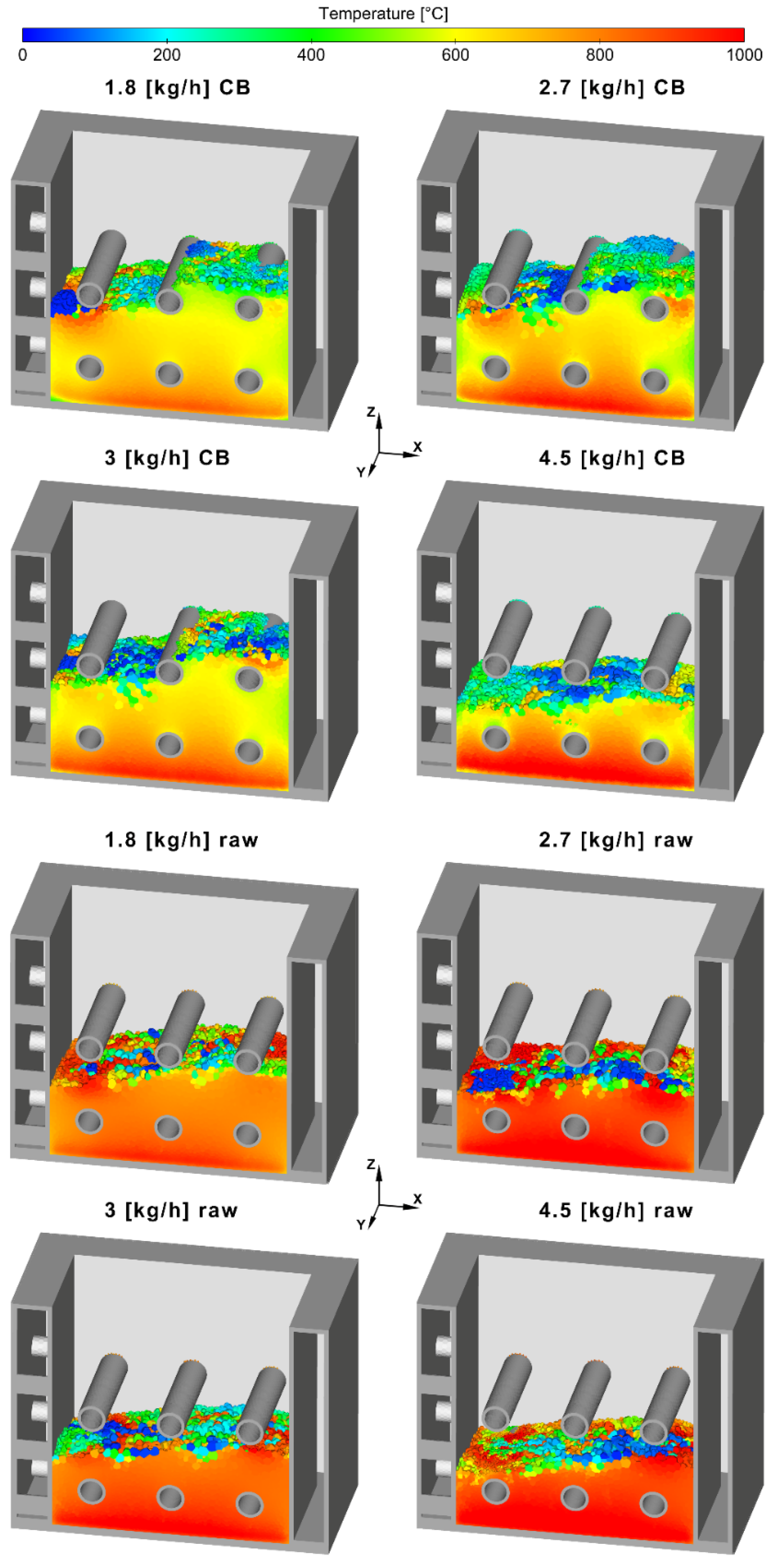
The bed temperature contours (Figure 7) confirm the effect of the bed cooling system on the average temperature of the solid fuel bed. In addition, it can be clearly seen how the increment of the primary air ratio increases the temperature of the solid fuel. These temperature variations affect the thermal conversion ratio of the biomass fuel, resulting in different bed thicknesses. The cases with lower primary air ratios tend to accumulate more fuel, due to the slower conversion rates caused by the lower flow of primary oxygen. Comparing the bed cooling and the raw cases with the same airflows, it can be seen that the cooled cases present larger bed volumes, due to lower conversion ratios caused by the temperature reduction.
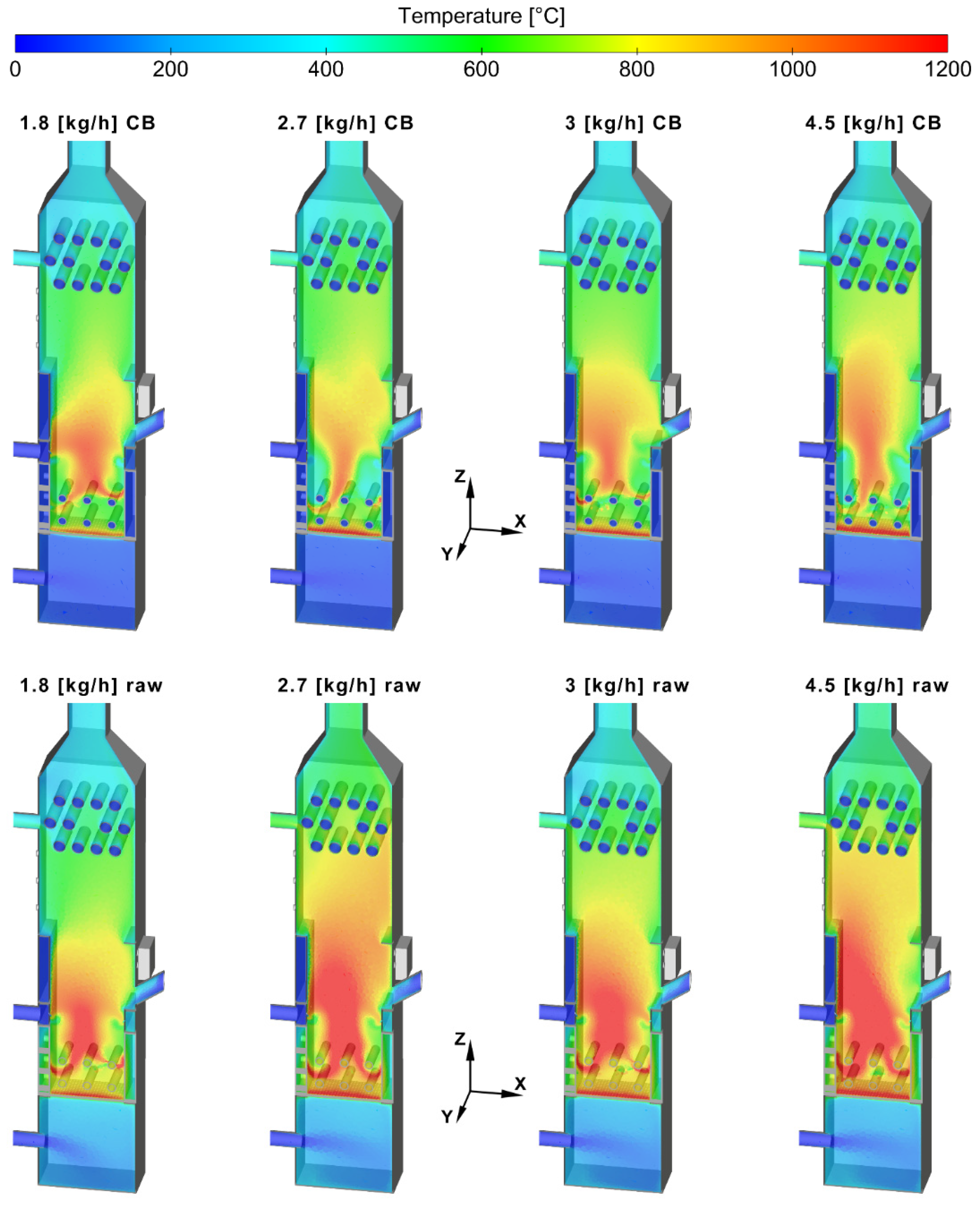
Figure 8 shows the temperatures of the gas phase and the water of the cooling circuits. It can be seen how the secondary air is injected toward the bed, and how the flame is started when this airflow encounters the volatile gases leaving the fuel bed. It can also be seen how the bed cooling and the different air ratios influence the gas temperature. The average temperature of the whole plant in the cooled bed cases is lower than in the raw cases. In addition, it can be easily seen in the raw cases that the 9 kg/h total airflow cases reach higher temperatures than in the 6 kg/h cases. This is a direct effect of the secondary airflow increase. This increases the turbulence and oxygen concentration in the combustion chamber, allowing for more complete combustion of the gases. The cases with higher secondary airflows, apart from higher temperatures in the gas phase, have also shown lower CO, CH4 and C6H6 emissions.
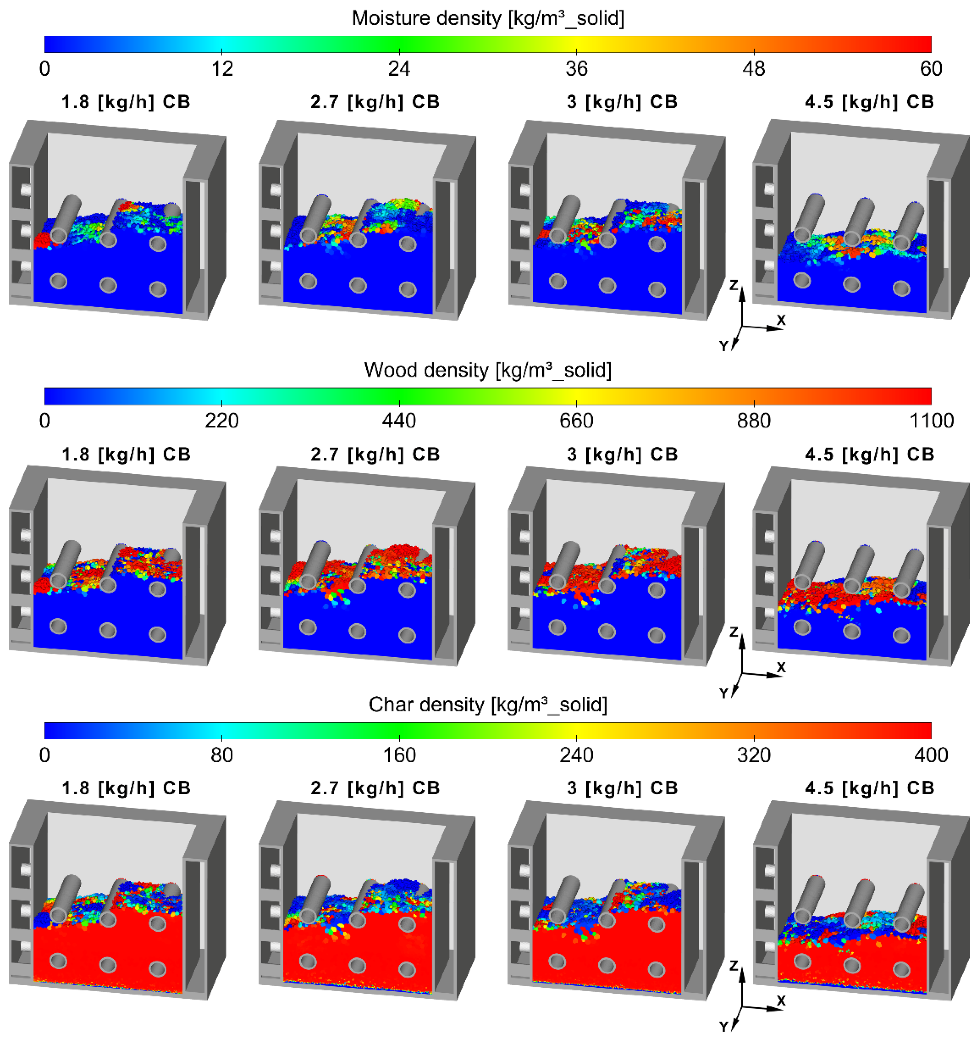
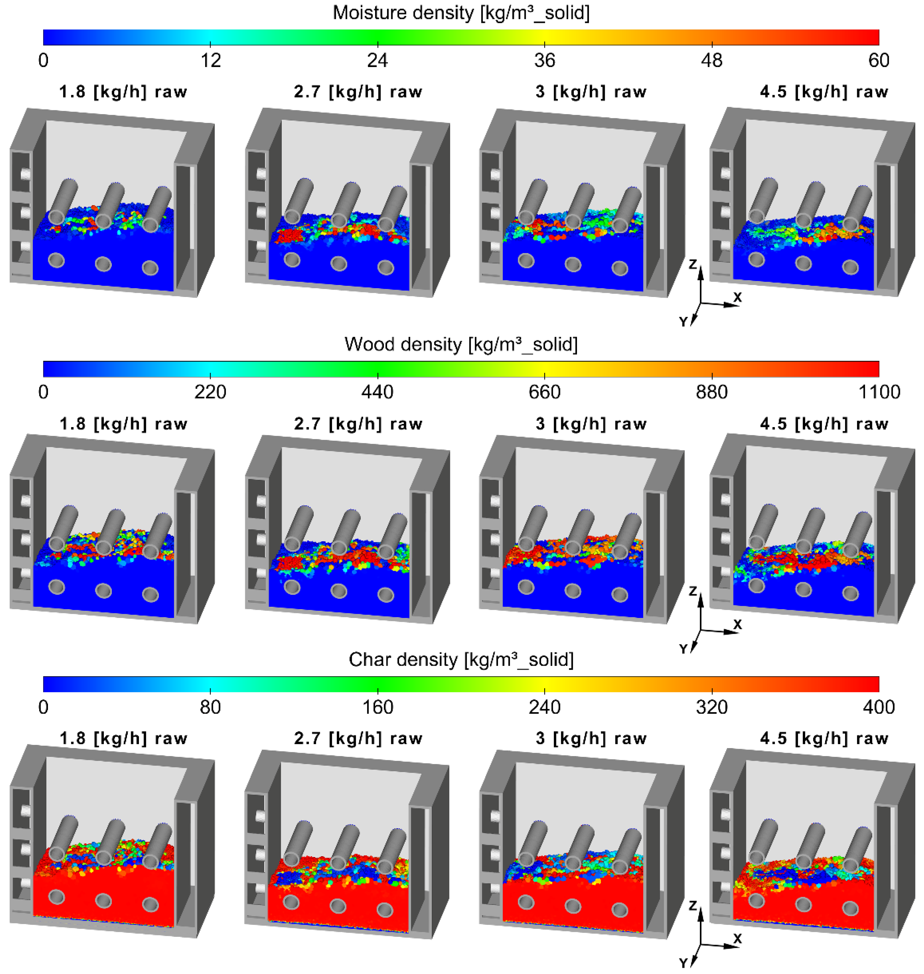
Figure 9 and Figure 10 show the solid bed densities of moisture, wood and char for the cooled bed cases and the raw cases, respectively. The most notable difference between cases is the thickness of the solid bed, the causes of which have already been discussed above. The bed is mostly composed of char, with the dry wood and wet fuel on top of the bed. The amount of moisture is similar in all cases, but the amount of dry wood is higher in the cooled bed cases because the lower bed temperatures slow down the wood pyrolysis, increasing its residence time.
In addition, it can be seen that the fresh fuel has a tendency to accumulate on the right side. This happens because the fuel is fed from an inlet located on the right side-wall of the combustion chamber module, which increases the chances of the particles falling closer to the right wall.
5. Conclusions
In this work, an experimental biomass fixed bed combustion plant, equipped with an internal bed cooling system, was numerically studied. A CFD commercial code and an Eulerian biomass thermal conversion model were used to carry out the simulations. Eight cases with different air ratios, and with the bed cooling system activated or not activated, were simulated to analyze the effect of air staging and bed cooling on the biomass thermal conversion processes. The obtained numerical results were compared against experimental results to validate the solution.
The CFD results showed good accordance with the experimental test measures. The bed model predicted maximum temperatures between 12% and 18% higher than the experimental values, and around 6% higher for the raw cases. The gas-phase measurements have a better adjustment, with an average deviation of around 8% for both bed-cooled and raw tests.
The bed cooling system reduces the bed temperatures by around 21%, and the gas temperatures around 12%, on average. This translates to an average reduction of 240 °C at the bed’s middle and upper zones. In the bottom zone, where the highest temperatures are recorded, the bed’s internal cooling system has less effect, due to the airflow going upward.
The air staging strategy has been proved effective in order to reduce bed temperatures. The direct relationship between the increase of the primary air ratio and the increment of bed temperatures has been predicted correctly. Because of this, in this type of system, it is advisable to work with low primary air ratios to reduce the bed temperatures and to reduce the PM elutriation. Air staging also helps to reduce the unburnt species emission, due to the increase of the secondary airflow.
The reduction of the bed’s average temperature help to reduce the number of inorganic alkali compounds volatilized, which are the main precursors of fouling and slagging over the refrigerated surfaces and of corrosion.
As futures lines of work, it would be interesting to study the slagging phenomena over the tubes of the internal bed cooling system and its influence on the heat transfer coefficients. The addition of a cooled grate in combination with the actual cooling system to reduce the maximum temperatures should also be taken into consideration. Regarding the modeling, in order to check the influence of the thermally thin assumption on the results, the simulations could be repeated using a thermally thick model that considers internal temperature gradients for the solid fuel bed particles. In addition, pollutant emissions modeling, such as PM and NOx formation mechanisms, could be implemented to study how the bed cooling and air staging strategies affect these phenomena.
Author Contributions
Conceptualization, C.Á.-B.; methodology, C.Á.-B., S.C. and M.Á.G.; software, C.Á.-B., S.C., L.G.V. and M.Á.G.; validation C.Á.-B., S.C., L.G.V. and M.Á.G.; formal analysis, C.Á.-B.; investigation, C.Á.-B., S.C., L.G.V. and M.Á.G.; resources, M.Á.G.; data curation, C.Á.-B.; writing—original draft preparation, C.Á.-B.; writing—review and editing, S.C., L.G.V. and M.Á.G.; visualization, C.Á.-B.; supervision, M.Á.G.; All authors have read and agreed to the published version of the manuscript.
Funding
This research was funded by the project RTI2018-100765-B-I00 of the Ministry of Science and Innovation (Spain). The work of César Álvarez-Bermúdez has been supported by the grant PRE2019-090110 of the Ministry of Science and Innovation (Spain).
Data Availability Statement
The data presented in this study is available in the current manuscript, raw data is available on request from the corresponding author.
Conflicts of Interest
The authors declare no conflict of interest. The funders had no role in the design of the study; in the collection, analyses, or interpretation of data; in the writing of the manuscript, or in the decision to publish the results.
References
- Sánchez, J.; Curt, M.D.; Robert, N.; Fernández, J. Biomass Resources. In The Role of Bioenergy in the Bioeconomy; Elsevier: Amsterdam, The Netherlands, 2019; pp. 25–111. [Google Scholar]
- Islas, J.; Manzini, F.; Masera, O.; Vargas, V. Solid Biomass to Heat and Power. In The Role of Bioenergy in the Bioeconomy; Elsevier: Amsterdam, The Netherlands, 2019; pp. 145–177. [Google Scholar]
- Patiño, D.; Pérez-Orozco, R.; Porteiro, J.; Lapuerta, M. Characterization of biomass PM emissions using thermophoretic sampling: Composition and morphological description of the carbonaceous residues. J. Aerosol Sci. 2019, 127, 49–62. [Google Scholar] [CrossRef]
- Rico, J.J.; Pérez-Orozco, R.; Cid, N.; Larrañaga, A.; Tabarés, J.L.M. Viability of Agricultural and Forestry Residues as Biomass Fuels in the Galicia-North Portugal Region: An Experimental Study. Sustainability 2020, 12, 8209. [Google Scholar] [CrossRef]
- Chapela, S.; Porteiro, J.; Gómez, M.A.; Patiño, D.; Míguez, J.L. Comprehensive CFD modeling of the ash deposition in a biomass packed bed burner. Fuel 2018, 234, 1099–1122. [Google Scholar] [CrossRef]
- Chapela, S.; Porteiro, J.; Garabatos, M.; Patiño, D.; Gómez, M.A.; Míguez, J.L. CFD study of fouling phenomena in small-scale biomass boilers: Experimental validation with two different boilers. Renew. Energy 2019, 140, 552–562. [Google Scholar] [CrossRef]
- Cai, Y.; Tay, K.; Zheng, Z.; Yang, W.; Wang, H.; Zeng, G.; Li, Z.; Boon, S.K.; Subbaiah, P. Modeling of ash formation and deposition processes in coal and biomass fired boilers: A comprehensive review. Appl. Energy 2018, 230, 1447–1544. [Google Scholar] [CrossRef]
- Chapela, S.; Cid, N.; Porteiro, J.; Míguez, J.L. Numerical transient modelling of the fouling phenomena and its influence on thermal performance in a low-scale biomass shell boiler. Renew. Energy 2020, 161, 309–318. [Google Scholar] [CrossRef]
- Chapela, S.; Porteiro, J.; Míguez, J.L.; Behrendt, F. CFD fouling model for fixed bed biomass combustion systems. Fuel 2020, 278, 118251. [Google Scholar] [CrossRef]
- Regueiro, A.; Patiño, D.; Porteiro, J.; Granada, E.; Míguez, J.L. Effect of air staging ratios on the burning rate and emissions in an underfeed fixed-bed biomass combustor. Energies 2016, 9, 940. [Google Scholar] [CrossRef] [Green Version]
- Khodaei, H.; Guzzomi, F.; Patiño, D.; Rashidian, B.; Yeoh, G.H. Air staging strategies in biomass combustion-gaseous and particulate emission reduction potentials. Fuel Process. Technol. 2017, 157, 29–41. [Google Scholar] [CrossRef]
- Archan, G.; Anca-Couce, A.; Buchmayr, M.; Hochenauer, C.; Gruber, J.; Scharler, R. Experimental evaluation of primary measures for NOX and dust emission reduction in a novel 200 kW multi-fuel biomass boiler. Renew. Energy 2021, 170, 1186–1196. [Google Scholar] [CrossRef]
- Pérez-Orozco, R.; Patiño, D.; Porteiro, J.; Rico, J.J. The effect of primary measures for controlling biomass bed temperature on PM emission through analysis of the generated residues. Fuel 2020, 280, 118702. [Google Scholar] [CrossRef]
- Pérez-Orozco, R.; Patiño, D.; Porteiro, J.; Larrañaga, A. Flue Gas Recirculation during Biomass Combustion: Implications on PM Release. Energy Fuels 2020, 34, 11112–11122. [Google Scholar] [CrossRef]
- Gómez, M.A.; Martín, R.; Chapela, S.; Porteiro, J. Steady CFD combustion modeling for biomass boilers: An application to the study of the exhaust gas recirculation performance. Energy Convers. Manag. 2019, 179, 91–103. [Google Scholar] [CrossRef]
- Gehrig, M.; Pelz, S.; Jaeger, D.; Hofmeister, G.; Groll, A.; Thorwarth, H.; Haslinger, W. Implementation of a firebed cooling device and its influence on emissions and combustion parameters at a residential wood pellet boiler. Appl. Energy 2015, 159, 310–316. [Google Scholar] [CrossRef]
- Gehrig, M.; Jaeger, D.; Pelz, S.K.; Kirchhof, R.; Thorwarth, H.; Haslinger, W. Influence of a Direct Firebed Cooling in a Residential Wood Pellet Boiler with an Ash-Rich Fuel on the Combustion Process and Emissions. Energy Fuels 2016, 30, 9900–9907. [Google Scholar] [CrossRef]
- Pérez-Orozco, R.; Patiño, D.; Porteiro, J.; Míguez, J.L. Novel Test Bench for the Active Reduction of Biomass Particulate Matter Emissions. Sustainability 2019, 12, 422. [Google Scholar] [CrossRef] [Green Version]
- Pérez-Orozco, R.; Patiño, D.; Porteiro, J.; Míguez, J.L. Bed cooling effects in solid particulate matter emissions during biomass combustion. A morphological insight. Energy 2020, 205, 118088. [Google Scholar] [CrossRef]
- Scharler, R.; Gruber, T.; Ehrenhöfer, A.; Kelz, J.; Bardar, R.M.; Bauer, T. CHochenauer, and A. Anca-Couce, Transient CFD simulation of wood log combustion in stoves. Renew. Energy 2020, 145, 651–662. [Google Scholar] [CrossRef]
- Zadravec, T.; Rajh, B.; Kokalj, F.; Samec, N. CFD modelling of air staged combustion in a wood pellet boiler using the coupled modelling approach. Therm. Sci. Eng. Prog. 2020, 20, 100715. [Google Scholar] [CrossRef]
- Buchmayr, M.; Gruber, J.; Hargassner, M.; Hochenauer, C. A computationally inexpensive CFD approach for small-scale biomass burners equipped with enhanced air staging. Energy Convers. Manag. 2016, 115, 32–42. [Google Scholar] [CrossRef]
- Wiese, J.; Wissing, F.; Höhner, D.; Wirtz, S.; Scherer, V.; Ley, U.; Behr, H.M. DEM/CFD modeling of the fuel conversion in a pellet stove. Fuel Process. Technol. 2016, 152, 223–239. [Google Scholar] [CrossRef]
- Somwangthanaroj, S.; Fukuda, S. CFD modeling of biomass grate combustion using a steady-state discrete particle model (DPM) approach. Renew. Energy 2020, 148, 363–373. [Google Scholar] [CrossRef]
- Rezeau, A.; Díez, L.I.; Royo, J.; Díaz-Ramírez, M. Efficient diagnosis of grate-fired biomass boilers by a simplified CFD-based approach. Fuel Process. Technol. 2018, 171, 318–329. [Google Scholar] [CrossRef]
- Bermúdez, C.A.; Porteiro, J.; Varela, L.G.; Chapela, S.; Patiño, D. Three-dimensional CFD simulation of a large-scale grate-fired biomass furnace. Fuel Process. Technol. 2020, 198, 106219. [Google Scholar] [CrossRef]
- Karim, M.R.; Bhuiyan, A.A.; Naser, J. Effect of recycled flue gas ratios for pellet type biomass combustion in a packed bed furnace. Int. J. Heat Mass Transf. 2018, 120, 1031–1043. [Google Scholar] [CrossRef]
- Karim, M.R.; Bhuiyan, A.A.; Sarhan, A.A.R.; Naser, J. CFD simulation of biomass thermal conversion under air/oxy-fuel conditions in a reciprocating grate boiler. Renew. Energy 2020, 146, 1416–1428. [Google Scholar] [CrossRef]
- Karim, M.R.; Naser, J. CFD modelling of combustion and associated emission of wet woody biomass in a 4 MW moving grate boiler. Fuel 2018, 222, 656–674. [Google Scholar] [CrossRef]
- Gómez, M.A.; Porteiro, J.; Patiño, D.; Míguez, J.L. CFD modelling of thermal conversion and packed bed compaction in biomass combustion. Fuel 2014, 117, 716–732. [Google Scholar] [CrossRef]
- Varela, L.G.; Bermúdez, C.Á.; Chapela, S.; Porteiro, J.; Tabarés, J.L.M. Improving Bed Movement Physics in Biomass Computational Fluid Dynamics Combustion Simulations. Chem. Eng. Technol. 2019, 42, 2556–2564. [Google Scholar] [CrossRef]
- ANSYS. ANSYS Fluent 2020 R1 Customization Manual; ANSYS: Canonsburg, PA, USA, 2020. [Google Scholar]
- Porteiro, J.; Collazo, J.; Patino, D.; Granada, E.; Gonzalez, J.C.M.; Miguez, J.L. Numerical Modeling of a Biomass Pellet Domestic Boiler. Energy Fuels 2009, 23, 1067–1075. [Google Scholar] [CrossRef]
- Collazo, J.; Porteiro, J.; Míguez, J.L.; Granada, E.; Gómez, M.A. Numerical simulation of a small-scale biomass boiler. Energy Convers. Manag. 2012, 64, 87–96. [Google Scholar] [CrossRef]
- Gómez, M.A.; Porteiro, J.; Patiño, D.; Míguez, J.L. Eulerian CFD modelling for biomass combustion. Transient simulation of an underfeed pellet boiler. Energy Convers. Manag. 2015, 101, 666–680. [Google Scholar] [CrossRef]
- Gómez, M.A.; Porteiro, J.; de la Cuesta, D.; Patiño, D.; Míguez, J.L. Numerical simulation of the combustion process of a pellet-drop-feed boiler. Fuel 2016, 184, 987–999. [Google Scholar] [CrossRef]
- Khodaei, H.; Gonzalez, L.; Chapela, S.; Porteiro, J.; Nikrityuk, P.; Olson, C. CFD-based coupled multiphase modeling of biochar production using a large-scale pyrolysis plant. Energy 2021, 217, 119325. [Google Scholar] [CrossRef]
- Varela, L.G.; Gómez, M.A.; Garabatos, M.; Glez-Peña, D.; Porteiro, J. Improving the bed movement physics of inclined grate biomass CFD simulations. Appl. Therm. Eng. 2021, 182, 116043. [Google Scholar] [CrossRef]
- Wagenaar, B.M.; Prins, W.; van Swaaij, W.P.M. Flash pyrolysis kinetics of pine wood. Fuel Process. Technol. 1993, 36, 291–298. [Google Scholar] [CrossRef] [Green Version]
- Thunman, H.; Leckner, B.; Niklasson, F.; Johnsson, F. Combustion of Wood Particles—A Particle Model for Eulerian Calculations. Combust. Flame 2002, 129, 30–46. [Google Scholar] [CrossRef]
- Bryden, K.M.; Ragland, K.W. Numerical Modeling of a Deep and Fixed Bed Combustor. Energy Fuels 1996, 10, 269–275. [Google Scholar] [CrossRef]
- Evans, D.D.; Emmons, H.W. Combustion of wood charcoal. Fire Saf. J. 1977, 1, 57–66. [Google Scholar] [CrossRef]
- Wakao, N.; Kaguei, S.; Funazkri, T. Effect of fluid dispersion coefficients on particle-to-fluid heat transfer coefficients in packed beds: Correlation of nusselt numbers. Chem. Eng. Sci. 1979, 34, 325–336. [Google Scholar] [CrossRef]
- Wakao, N.; Funazkri, T. Effect of fluid dispersion coefficients on particle-to-fluid mass transfer coefficients in packed beds: Correlation of sherwood numbers. Chem. Eng. Sci. 1978, 33, 1375–1384. [Google Scholar] [CrossRef]
- Gómez, M.A.; Patiño, D.; Comesaña, R.; Porteiro, J.; Feijoo, M.A.Á.; Míguez, J.L. CFD simulation of a solar radiation absorber. Int. J. Heat Mass Transf. 2013, 57, 231–240. [Google Scholar] [CrossRef]
- Chapela, S.; Porteiro, J.; Costa, M. Effect of the Turbulence–Chemistry Interaction in Packed-Bed Biomass Combustion. Energy Fuels 2017, 31, 9967–9982. [Google Scholar] [CrossRef]
- Thunman, H.; Niklasson, F.; Johnsson, F.; Leckner, B. Composition of Volatile Gases and Thermochemical Properties of Wood for Modeling of Fixed or Fluidized Beds. Energy Fuels 2001, 15, 1488–1497. [Google Scholar] [CrossRef]
- Anca-Couce, A. Reaction mechanisms and multi-scale modelling of lignocellulosic biomass pyrolysis. Prog. Energy Combust. Sci. 2016, 53, 41–79. [Google Scholar] [CrossRef]
- Jones, W.P.; Lindstedt, R.P. Global Reaction Schemes for Hydrocarbon Combustion. Combust. Flame 1988, 73, 233–249. [Google Scholar] [CrossRef]
- Andersen, J.; Jensen, P.A.; Meyer, K.E.; Hvid, S.L.; Glarborg, P. Experimental and Numerical Investigation of Gas-Phase Freeboard Combustion. Part 1: Main Combustion Process. Energy Fuels 2009, 23, 5773–5782. [Google Scholar] [CrossRef]
Figure 1.
Mid cuts of the internally cooled biomass combustion plant.

Figure 2.
Positions of the thermocouples (red tip) inside the system, and detail of the bed zone.

Figure 3.
Detail of the mesh mid-cut in the bed zone.

Figure 4.
Numerical versus experimental temperature profiles of the raw bed tests.

Figure 5.
Numerical versus experimental temperature profiles of the cooled bed tests.

Figure 6.
Comparison of the temperature profiles of the CFD cases.

Figure 7.
Bed temperature contours for both the cooled and the raw beds.

Figure 8.
Contours of gas temperature in the mid-plane (y = 0).

Figure 9.
Solid bed densities—contours of the bed-cooled cases.

Figure 10.
Solid bed densities—contours of the raw cases.


Table 1.
Transport equations of the solid phase scalars.
| Solid temperature | (1) | |
| Solid fraction | (2) | |
| Particle diameter | (3) | |
| Moisture density | (4) | |
| Wood density | (5) | |
| Char density | (6) | |
| Ash density | (7) |
Table 2.
Solid consumption rate equations.
| Drying rate | (8) | |
| Devolatilization rate | (9) | |
| Char consumption rate | (10) |
Table 3.
Kinetics of the solid heterogeneous reactions.
| Pyrolysis Reactions | Ai (s−1) | Ei (kJ/mol) | References |
| Dry wood → Gas | 1.11 × 10¹¹ | 177 | [39] |
| Dry wood → Tar | 9.28 × 10⁹ | 149 | [39] |
| Dry wood → Char | 3.05 × 10⁷ | 125 | [39] |
| Char Reactions | Kinetics | References | |
| [40,41] | |||
| [40,41] | |||
| [41] | |||
Table 5.
Fuel characterization [19].
Table 5.
Fuel characterization [19].
| Proximate Analysis a | [wt%] |
| Moisture | 5.23 |
| Volatile | 71.57 |
| Fixed carbon | 22.81 |
| Ash | 0.39 |
| Ultimate Analysis b | [wt%] |
| C | 47.21 |
| H | 6.34 |
| O | 45.96 |
| N | 0.08 |
| Heating Values a | [MJ/kg] |
| HHV | 18.19 |
| LHV | 16.74 |
a wet basis, as received. b dry basis, ash-free.
Table 6.
Control variables defining the experiment sets [19].
Table 6.
Control variables defining the experiment sets [19].
| Test Name | Total Airflow [kg/h] | Primary Air Ratio [%] | Bed Cooling |
|---|---|---|---|
| 1.8 [kg/h] raw | 6 | 30 | OFF |
| 2.7 [kg/h] raw | 9 | 30 | OFF |
| 3 [kg/h] raw | 6 | 50 | OFF |
| 4.5 [kg/h] raw | 9 | 50 | OFF |
| 1.8 [kg/h] CB | 6 | 30 | ON |
| 2.7 [kg/h] CB | 9 | 30 | ON |
| 3 [kg/h] CB | 6 | 50 | ON |
| 4.5 [kg/h] CB | 9 | 50 | ON |
Publisher’s Note: MDPI stays neutral with regard to jurisdictional claims in published maps and institutional affiliations. |
© 2021 by the authors. Licensee MDPI, Basel, Switzerland. This article is an open access article distributed under the terms and conditions of the Creative Commons Attribution (CC BY) license (https://creativecommons.org/licenses/by/4.0/).
Share and Cite
MDPI and ACS Style
Álvarez-Bermúdez, C.; Chapela, S.; Varela, L.G.; Gómez, M.Á. CFD Simulation of an Internally Cooled Biomass Fixed-Bed Combustion Plant. Resources 2021, 10, 77. https://0-doi-org.brum.beds.ac.uk/10.3390/resources10080077
AMA Style
Álvarez-Bermúdez C, Chapela S, Varela LG, Gómez MÁ. CFD Simulation of an Internally Cooled Biomass Fixed-Bed Combustion Plant. Resources. 2021; 10(8):77. https://0-doi-org.brum.beds.ac.uk/10.3390/resources10080077
Chicago/Turabian StyleÁlvarez-Bermúdez, César, Sergio Chapela, Luis G. Varela, and Miguel Ángel Gómez. 2021. "CFD Simulation of an Internally Cooled Biomass Fixed-Bed Combustion Plant" Resources 10, no. 8: 77. https://0-doi-org.brum.beds.ac.uk/10.3390/resources10080077
Note that from the first issue of 2016, this journal uses article numbers instead of page numbers. See further details here.