Article

Surplus Cost Potential as a Life Cycle Impact Indicator for Metal Extraction

by
Marisa D.M. Vieira
1,2,*,
Thomas C. Ponsioen
2,
Mark J. Goedkoop
2 and
Mark A.J. Huijbregts
1
1
Radboud University Nijmegen, Faculty of Science, Department of Environmental Science, P.O. Box 9010, Nijmegen 6500 GL, The Netherlands
2
PRé Consultants b.v., Stationsplein 121, Amersfoort 3818 LE, The Netherlands
*
Author to whom correspondence should be addressed.
Submission received: 28 October 2015 / Revised: 20 December 2015 / Accepted: 22 December 2015 / Published: 6 January 2016
(This article belongs to the Special Issue Consideration of Abiotic Natural Resources in Life Cycle Assessments)

Abstract

:
In the evaluation of product life cycles, methods to assess the increase in scarcity of resources are still under development. Indicators that can express the importance of an increase in scarcity of metals extracted include surplus ore produced, surplus energy required, and surplus costs in the mining and the milling stage. Particularly the quantification of surplus costs per unit of metal extracted as an indicator is still in an early stage of development. Here, we developed a method that quantifies the surplus cost potential of mining and milling activities per unit of metal extracted, fully accounting for mine-specific differences in costs. The surplus cost potential indicator is calculated as the average cost increase resulting from all future metal extractions, as quantified via cumulative cost-tonnage relationships. We tested the calculation procedure with 12 metals and platinum-group metals as a separate group. We found that the surplus costs range six orders of magnitude between the metals included, i.e., between $0.01–$0.02 (iron) and $13,533–$17,098 (rhodium) USD (year 2013) per kilogram of metal extracted. The choice of the reserve estimate (reserves vs. ultimate recoverable resource) influenced the surplus costs only to a limited extent, i.e., between a factor of 0.7 and 3.2 for the metals included. Our results provide a good basis to regularly include surplus cost estimates as resource scarcity indicator in life cycle assessment.

Graphical Abstract

1. Introduction

The need for reduction of greenhouse gas emissions will most likely shift energy generation from fossil fuels to alternative sources of energy such as solar, wind and nuclear power [1]. Renewable energy production technologies often require significantly more metals in their construction, such as copper, indium, lead, and molybdenum, compared to fossil energy [2]. It is, therefore, important to understand the trade-offs in using different types of mineral, metal, and fossil resources. Life cycle assessment (LCA) is a method that is capable of quantifying trade-offs in terms of potential impacts on human health, natural environment and natural resources [3]. Particularly, life cycle impact assessment (LCIA) methods assessing impacts on natural resources are still in an early stage of development [4,5,6].
Many indicators previously developed for resource use in LCA focused on evaluating the exhaustion of resources in the earth. Tilton [7] defined this as the fixed stock paradigm, which implies that resources are limited and will eventually deplete. However, physical availability is most likely not the main problem as many metals are not destroyed after their use, but their economic availability is [8,9,10,11,12]. Even though there may be commodities available to mine in the Earth’s crust, the cost of extraction can be higher than the price consumers are willing to pay [7,9,10,11,12,13,14]. For fossil resources the same is observed, with costs being the limiting factor for fossil resource extraction [15]. Since costs appear to be the limiting factor for the use of both metal and fossil resources, a resource scarcity indicator expressed in costs for these resources is considered worthwhile to investigate [11,12,16,17,18,19].
The European Commission-Joint Research Centre—Institute for Environment and Sustainability [5] indicated surplus costs, as explored by the ReCiPe method [20], as a promising indicator to assess resource use among the existing approaches. However, its application is not yet considered mature for recommendation [5]. For instance, mining and milling costs per unit of ore extracted were considered constant across all mines [20]. Surplus costs are defined as the (economic) burden that current resource extraction puts on future situations. These surplus costs over a long period of time are not particularly considered in current decision making [10]. This definition closely links up with the focus on externalities in LCA, i.e., the cost that affects a party who did not choose to incur that cost [21,22]. The quantification of these external costs directly fit into the framework of environmental life cycle costing (LCC) [23,24].
The goal of this paper was to develop a method that quantifies the surplus cost potential per unit of metal extracted in the future, fully accounting for co-production and mine-specific differences in costs. We demonstrated how the method can be applied in practice for 12 metal commodities including uranium, which is also an energy resource, and platinum-group metals as a group.

2. Methods and Data

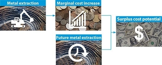
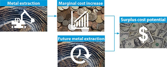
2.1. Cause-Effect Pathway

Metals may come from two origins, either from mining or from secondary production, the latter resulting from waste recovery. The current fraction of secondary production has to be included in the life cycle inventory and is therefore not considered in the LCIA step. Without technological development in the mining industry, increased primary metal extraction results in a subsequent increase in mining and milling costs, as mines with lower operating costs are explored first. The operating costs account for co-production and are allocated across all mine products in proportion to their revenue to the mine operator. The average cost increase resulting from all future extraction of a metal is calculated to arrive at the surplus costs per unit of metal extracted.

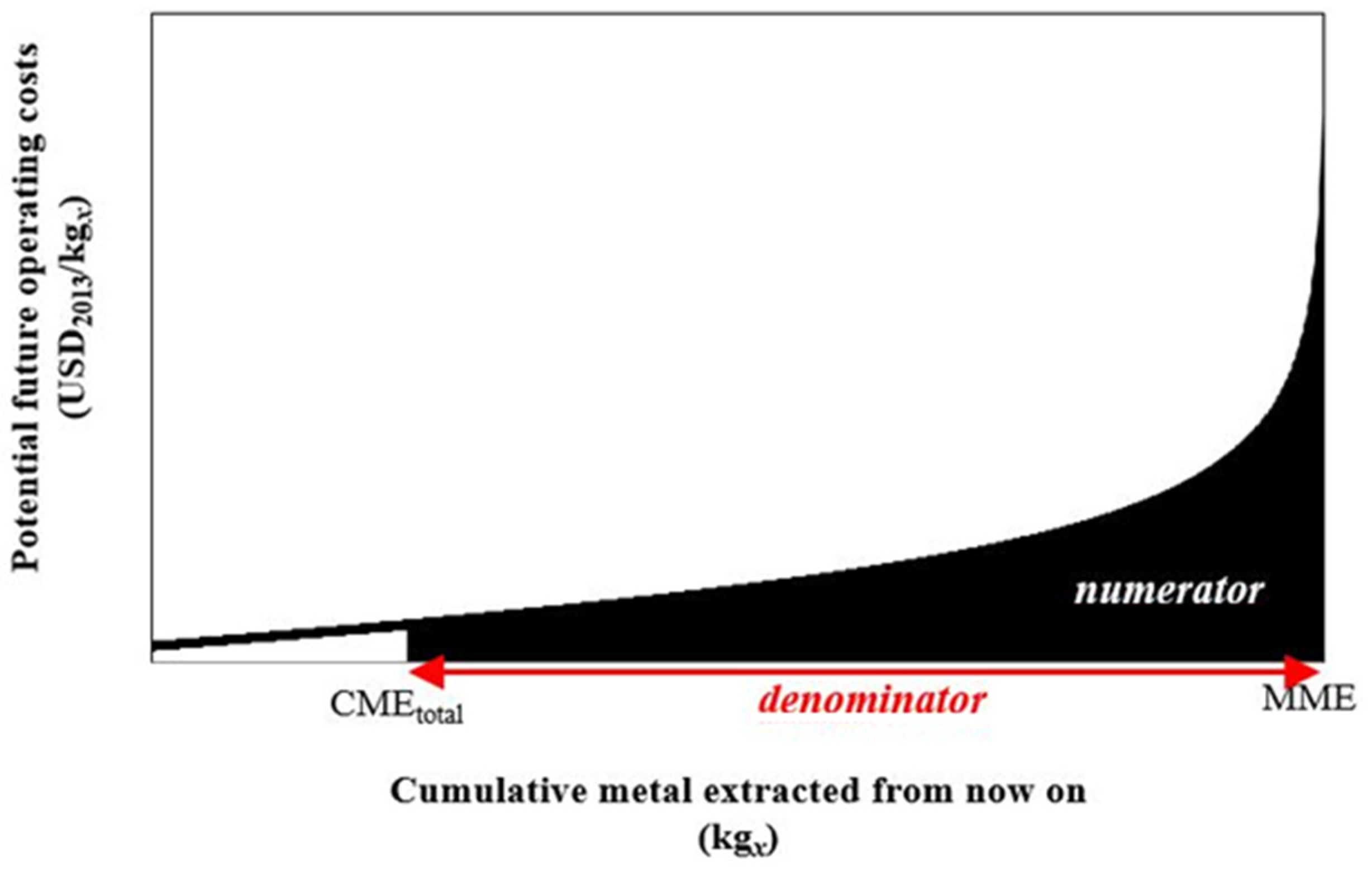
2.2. Cumulative Cost-Tonnage Relationships

Following the principle that mining sites with lower costs are the first to be explored, mines producing a certain metal were sorted by increasing order of costs per metal extracted. Vieira et al. [25] demonstrated that ore grades tend to decrease with the increase of copper extraction and that a log-logistic regression can be applied to cumulative grade-tonnage relationships. Following the same line of reasoning for costs, a log-logistic distribution can be fitted on the inverse of operating costs per metal extracted and the cumulative metal extracted to account for the skewness in the data points [25] by:
1 C x = exp ( α x ) · exp ( β x · ln ( A x , sample CME x , sample CME x , sample ) )
where Cx is the operating cost per metal x produced (in USD/kgx), αx is the scale parameter, and βx is the shape parameter of the log-logistic distribution, and Ax,sample and CMEx,sample (both in kgx) are, respectively, the total metal x extracted and the cumulative metal x extracted for the data sample used to derive the curve.

2.3. Characterization Factors

The surplus cost potential per unit of extraction of a metal is an indicator of the future economic scarcity of the extraction of this resource. The characterization factor (CF), defined as the average Surplus Cost Potential (SCP) of metal x, was calculated by:
CF x = CME x , total MME x C x ( ME x ) d ME x R x = CME x , total MME x C x ( ME x )   d ME x MME x CME x , total
where Cx is the operating cost determined via the cumulative cost-tonnage curve of metal x for an amount of metal x extracted (MEx), Rx (kgx) is the reserve of metal x, defined as the difference between all current known cumulative tonnage of metal x extracted (CMEx,total) and the global maximum tonnage of metal x ever extracted (MMEx). This is illustrated in Figure 1.
Figure 1. Visualization of the derivation of the surplus cost potential following an average approach and a log-logistic cumulative cost-tonnage curve from the current cumulative metal extracted (CMEtotal) up to global maximum metal extracted (MME).
Resources 05 00002 g001
The overall surplus cost potential caused by a product, e.g., production of photovoltaic electricity in Spain, can be calculated by:
IS nr = x CF x × M x
where ISnr is the impact score of natural resource extraction per functional unit of the product analyzed, e.g., production of 1 kWh of photovoltaic electricity in Spain (USD/kWh solar electricity); CFx is the characterization factor for resource x extracted (USD/kgx); and Mx is the amount of resource x extracted per functional unit (e.g., kgx/kWh solar electricity). This impact score is measured at the endpoint level, thus measuring the potential damage caused, and aggregates the impact score of various types of abiotic natural resources, namely metal, mineral, and fossil resources.

2.4. Sensitivity Analysis

Alternative scenarios were calculated and analyzed with regards to the future production of metals. Since it is unclear what the exact future production of each metal will be, reserves data were used. Reserves data are variable because, on the one hand, ores are constantly being explored and the extraction feasibility may decrease and, on the other hand, new deposits are being discovered or become economically viable. To study the uncertainty of the future production of metals two different reserve estimates were applied. The first type of reserve estimate is the “Reserves (RR)” which is defined as that part of a mineral resource “which could be economically extracted or produced at the time of determination”, meaning at current prices, state of technology, etc. [26]. The other type of reserve estimate, the “ultimate recoverable resource (RURR)”, refers to “the amount available in the upper earth’s crust that is ultimately recoverable”. The definition of ultimate recoverable resource as used by UNEP [27], there called extractable global resource (EGR), was used here. This is assuming that 0.01% of the total amount in the crust to 3 km depth will ultimately be available.

2.5. Data Selection and Fitting

Characterization factors were derived for copper (Cu), iron (Fe), lead (Pb), manganese (Mn), molybdenum (Mo), nickel (Ni), palladium (Pd), platinum (Pt), rhodium (Rh), silver (Ag), uranium (U), zinc (Zn), and for platinum-group metals (PGM) as a group. Table 1 shows the data for the metals included in the calculation of the characterization factors.
Table 1. Global cumulative extraction and reserve estimates used for deriving the characterization factors expressed as surplus cost potential [26,27,28,29,30,31,32].
MetalCumulative Metal ExtractedMaximum Metal Extracted
CMEtotal (kgx)MMER (kgx)MMEURR (kgx)
Copper5.92 × 10111.28 × 10125.22 × 1012
Iron3.41 × 10131.15 × 10146.49 × 1015
Lead2.35 × 10113.24 × 10113.04 × 1012
Manganese5.80 × 10111.15 × 10121.28 × 1014
Molybdenum6.62 × 1091.76 × 10101.89 × 1011
Nickel5.53 × 10101.29 × 10117.82 × 1012
Palladium5.15 × 1062.83 × 1078.25 × 107
Platinum6.97 × 1063.82 × 1071.12 × 108
Rhodium7.36 × 1054.04 × 1061.18 × 107
Silver1.13 × 1091.65 × 1092.11 × 1010
Uranium2.71 × 1095.23 × 1094.33 × 1011
Zinc4.58 × 10117.08 × 10111.16 × 1013
Platinum-Group Metals1.47 × 1078.07 × 1072.36 × 108

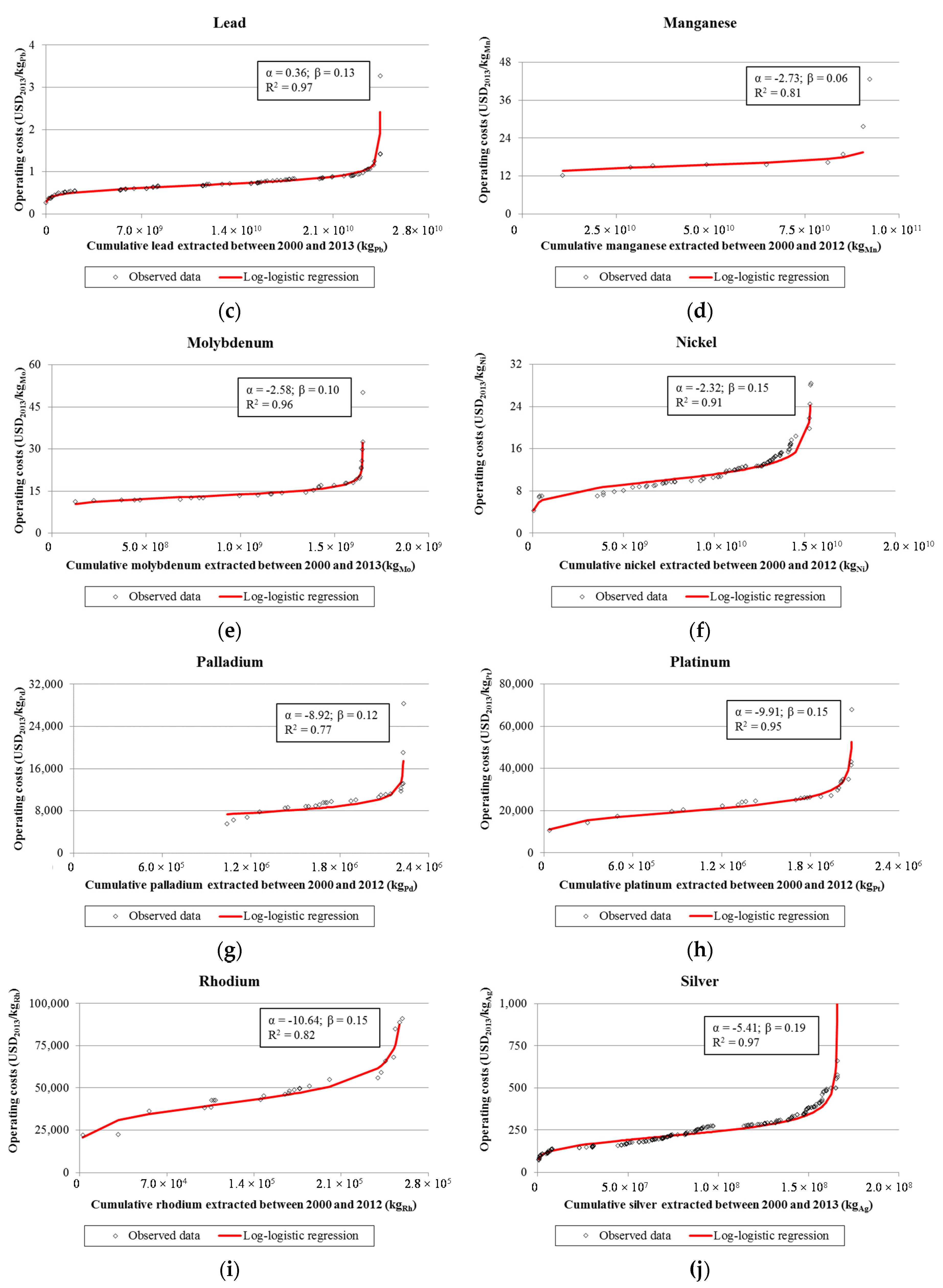
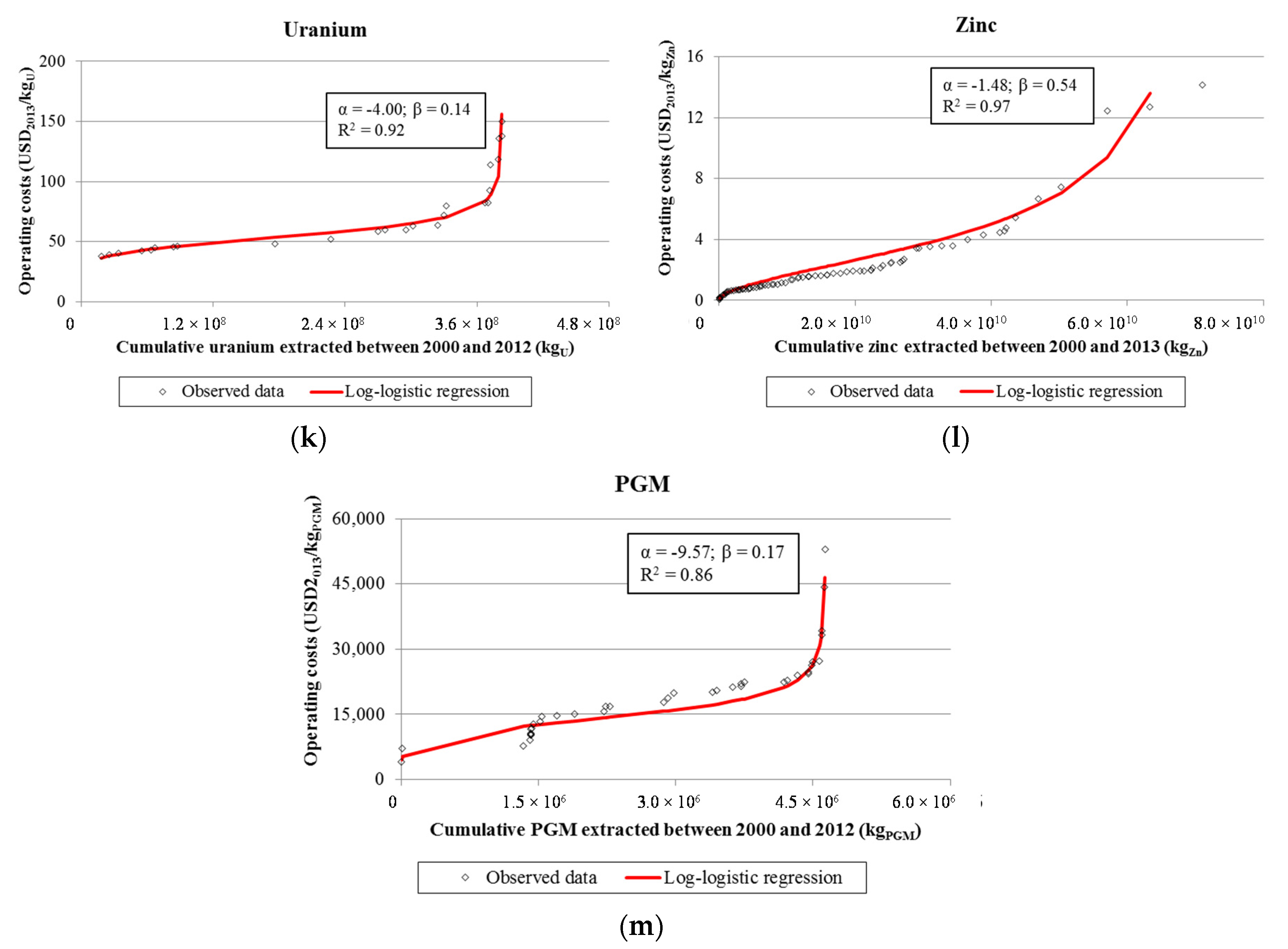
2.5.1. Cumulative Cost-Tonnage Relationships

To derive log-logistic cumulative cost-tonnage relationships, yearly metal production (in kgx) and mining and milling costs per metal produced data (in USD/kgx) between 2000 and 2013 were purchased from the World Mine Cost Data Exchange (WMCDE) [33]. The database contained for each metal one cost curve per year with production and cost data for each mine. The data used for deriving the cumulative cost-tonnage relationships are presented in Table S1 in the Supplementary Material.
The log-logistic distribution for each metal was derived as follows:
-
Typically, deposits contain various metals but there is often a main metal that justifies the operation of a mine exploring that deposit. As such, the operating costs of a mine are to be shared by all outputs with a market value. In the World Mine Cost Data Exchange [33], the costs were allocated across all mine products in proportion to their production (monetary) value to the mine operator.
-
Each table includes data in U.S. dollars valued in the year it represents, e.g., the costs for 2004 are expressed in constant USD valued in 2004. The CPI Inflation Calculator [34] was used to convert all costs into U.S. dollars for 2013 (USD2013).
-
For each mine, the weighted average costs per amount of metal produced, calculated on basis of the operating costs per metal in that mine each year and the production tonnages for the same years, and the total metal extracted in the period covered for that mine were calculated.
-
The mines were then ranked in increasing order of costs per amount of metal extracted and the cumulative metal extracted for each mine was calculated by adding the metal extracted of that mine to that of all previous mines with lower operating costs.
-
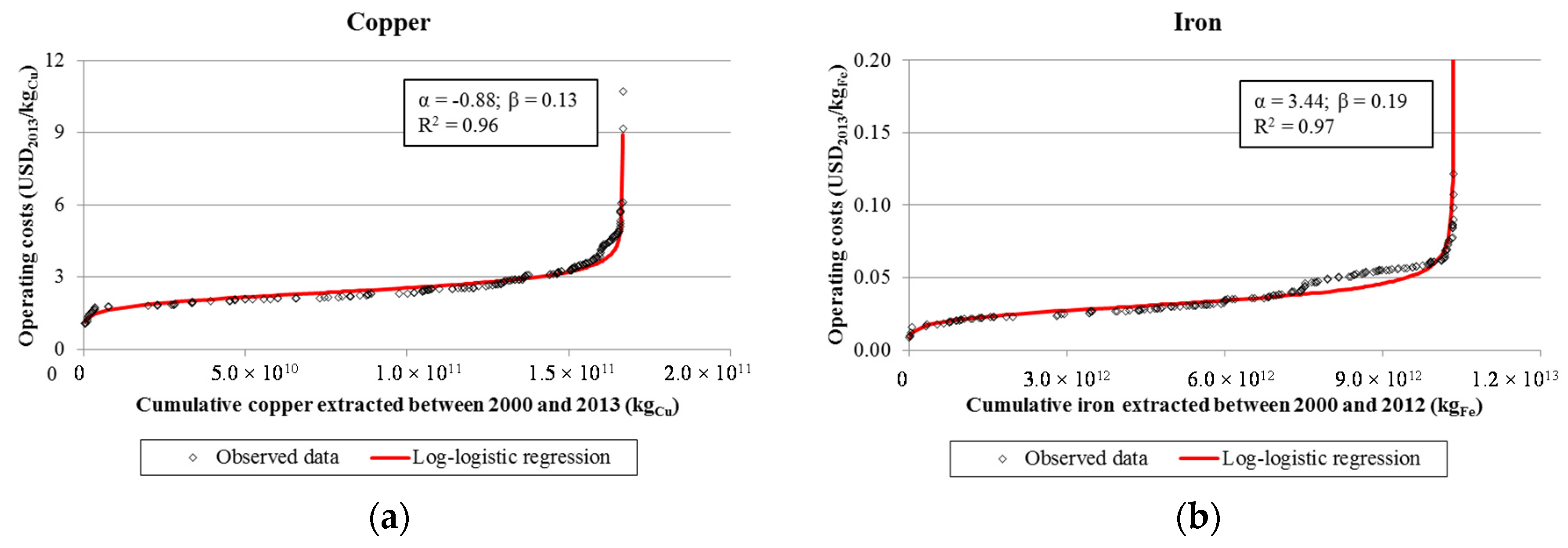
A log-logistic fit was applied to the inverted costs for every mine with the software R for statistical computing [35] to derive the scale parameter α and the shape parameter β, including their 95% confidence interval (95% CI). The R square (R2) of the log-logistic fit was also determined. For the derivation of α and β, the total tonnage of metal extracted Ax was set equal to the total metal extracted as reported in the WMCDE database between 2000 and 2012 or 2013, depending on the metal [33].

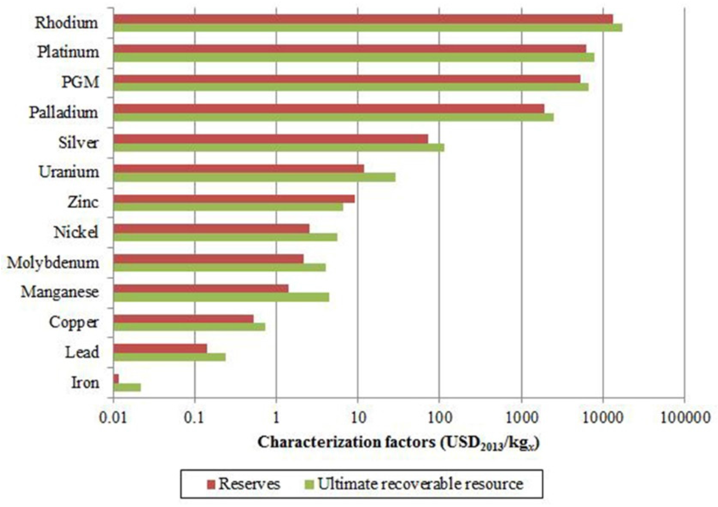
2.5.2. Characterization Factors

To derive the surplus cost potential per metal x, the cumulative metal extracted up to now (CMEx,total) is calculated as the total production from Kelly and Matos [28] which contains world mine production tonnage since 1900 until 2012 for every metal under study except for uranium. For uranium, data was retrieved from Nuclear Energy Agency and International Atomic Energy Agency [29].
To calculate the maximum amount of metal x extracted (MMEx), global reserve estimates for each metal are required. As mentioned above, two types of reserves were used: reserves and ultimate recoverable resource. Reserves were set equal to the global mineral reserves as specified by the U.S. Geological Survey [26]. U.S. Geological Survey [26] estimated the reserves for all metals under study, except for the individual platinum-group metals (PGM) and uranium. For uranium, the global reserves, following the same definition, were taken from Hall and Coleman [30]. Reserves fraction of platinum (47.3%), palladium (35.0%), and rhodium (5.0%) were calculated from data for the three PGM ore types mined in the Bushveld deposit situated in South Africa which accounts for nearly 90 percent of PGM’s reserves [31].
Schneider et al. [32] estimated the ultimate recoverable resource (URR) for 19 metals and for PGM as a group, eight of which are relevant for this study. The URR data for silver and uranium, following the same definition, was taken from UNEP [27]. The data used for the two types of reserves are presented in Table S2 in the Supplementary Material.

3. Results

3.1. Cumulative Cost-Tonnage Relationships

Figure 2 shows the log-logistic relationships between cumulative extraction of metal x and increase in operating costs per unit of metal x. A number of metals (copper, lead, manganese, molybdenum, nickel, palladium, platinum) and PGM indicate relatively high costs with low production for a few mines. This can be seen from Figure 2, as a few data points on the right hand side of the curve are almost in a vertical line, meaning low production tonnage and at the same time substantially higher costs compared to other mines. These costs often result from co-production in which the main metal being extracted is another than the one under study. Taking Figure 2a for copper as an example, the mine with the highest cost per kilogram of copper extracted is Copper Rand in Canada, with gold and silver as co-products [33]. Since 2009, this mine has been closed due to high costs in comparison with the low copper prices [36]. However, if prices rise this mine may be reopened. This effect is in line with the method here proposed in which mines with lower operating costs per output of metal are extracted first.
The log-logistic fit between costs and cumulative extraction of a metal resulted in explained variances between 77% (for palladium) and 97% (for iron, lead, silver, and zinc). The parameters derived for the log-logistic cost-tonnage relationships are presented in Table S3 in the Supplementary Material.
Figure 2. Cumulative cost-tonnage relationships and scale α and shape β derived with the log-logistic distribution for copper (a), iron (b), lead (c), manganese (d), molybdenum (e), nickel (f), palladium (g), platinum (h), rhodium (i), silver (j), uranium (k), zinc (l), and platinum-group metals (m). The data were taken from the World Mine Cost Data Exchange [33] for the period from 2000 to 2012/2013.
Resources 05 00002 g002aResources 05 00002 g002bResources 05 00002 g002c

3.2. Characterization Factors

The characterization factors derived for the metals under study are presented in Figure 3 and can also be found in Table S4 in the Supplementary Material. The CFs obtained vary up to six orders of magnitude. Rhodium resulted in the highest CF of $13,533–$17,098 USD2013 per kg of rhodium extracted, while the lowest CF derived was for iron with $0.01–$0.02 USD2013 per kg of iron extracted.
With the exception of zinc, the surplus cost potentials derived are always largest using ultimate recoverable resource compared to using the reserves. The CF depends on the combination of the scale parameter (α), the shape parameter (β), CME, and MME of a metal. It is not necessarily true that that the CF gets always higher when MME becomes larger. In fact with very small MME values, so very low reserves, the starting point of the cumulative cost calculation (CMEtotal) is in the steepest part of the curve and the CFs become very large. This means that getting the last amount of metal out of the ground will be very costly. Applying ultimate recoverable resource instead of reserves always result in a lower fraction mined of the total amount available another working point. For instance, for copper 46% of the total amount is already mined using reserves, while 11% is mined according to ultimate recoverable resources. For zinc this is 56% versus 4%. Depending on the shape (β) of the log-logistic curve (relatively steep for copper and relative shallow for zinc), the increase in costs over the full amount of metal mined can be larger or lower. In this case, the average steepness of the cost curve for copper is larger for 11% to 100% metal extracted compared to 46% to 100%. In contrast, the average steepness of the cost curve for zinc is larger for 56% to 100% metal extracted compared to 4% to 100%.
Figure 3. Characterization factors expressed as surplus cost potential (USD2013/kgx extracted) using reserves and ultimate recoverable resource as future extraction estimates.
Resources 05 00002 g003

4. Discussion

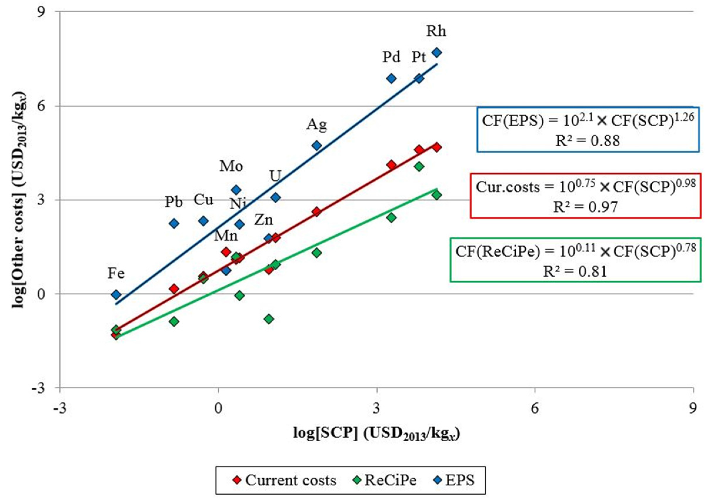
4.1. Comparison with other Indicators

Although log-logistic functions can be applied to derive both cumulative cost and ore grade curves, the exact causal relationship between ore grade decrease and surplus costs is unknown as far as we know of. Though ore grade can be considered as an important factor for determining the operating costs in a mine [37], other factors that change over time can be important as well. These are further discussed in the Limitations section.
For all metals under study the current operating costs were derived, calculated as the weighted average operating costs of all mines for 2013 on basis of their yearly production of that metal, from the World Mine Cost Data Exchange [33]. Goedkoop and De Schryver [20] derived characterization factors in the ReCiPe method expressed as surplus costs following a simplified approach of the method here proposed, e.g., with mining and milling costs per unit of ore considered constant across all mines. Steen [38] derived characterization factors in the method to environmental priority strategies for product development (EPS), defined as the costs to be paid to extract the mineral resources using future technologies. For this method, a market scenario was created, where all future generations are included and are imagined to bid on the present abiotic stock reserves [38]. All three monetary results per metal can be seen in Table S5 in the Supplementary Material.
In Figure 4, the current operating costs, the CFs derived in the ReCiPe method with 3% discounting, and the CFs derived in the EPS method are compared to the CFs here derived using reserves as reserve estimate. For all metals except for zinc, the current operating costs are larger than the surplus costs derived here. There is a factor difference of between 0.7 for zinc and a factor of about 16 for manganese. From the log-linear regression in Figure 4, it can be seen that the surplus cost potentials will be about 5.6 (equal to the intercept of the regression) times lower than its current operating costs.
According to the log-linear regression derived in Figure 4 the CFs here derived give typically a factor of 1.3 lower CFs compared to the ReCiPe method with a coefficient of determination (R2) of 0.81. Note that for individual metals, the differences between the two methods can be much larger, i.e., a factor of seven lower for molybdenum and a factor of 57 higher for zinc in our study compared to the Goedkoop and De Schryver [20] method.
Compared to the EPS method, the CFs derived here give on average a factor of 126 lower with a coefficient of determination (R2) of 0.88 (see log-linear regression in Figure 4). The differences between the CFs derived by each method for individual metals can differ to up to four orders of magnitude, i.e., a factor of four for manganese and of 4 × 10³ for palladium.
Figure 4. Log-linear relationship between the characterization factors (SCP) here derived, current operating costs [33], the CFs derived in the ReCiPe method [20], and the CFs derived in the EPS method [38]. Both axis are presented in logarithmic scale.
Resources 05 00002 g004

4.2. Limitations

Although we improved the surplus cost calculations of metals compared to current practice, there are still limitations in our calculations as we assumed that costs increase with the increase of metal extracted without explicitly considering the mine type, ore type, new discoveries and technological developments. Currently, open pit mining is preferred due to lower operational costs even though underground mines often contain higher metal grades [39,40,41]. As open pit mines will most likely become depleted in the future, a shift towards underground mining is likely to occur. Gerst [42] estimated that mining operations have to become deeper than the current open pit mining operations. Furthermore, different ores have different characteristics and moving from one to the other may result in substantially different mining conditions and, as a result, in different operating costs [43]. The cost and tonnage data used to derive the cumulative cost-tonnage curves, however, does not contain information on the mine type and ore type. This is why we did not separately derive cumulative cost-tonnage curves for open pit and underground mines and different ore types in our study. Additionally, there is evidence of overall reduction in mining costs per amount of ore extracted due to technological advances in the mining sector [39,44]. For instance, mines have been increasing in size and the larger the mine size the lower the costs per output extracted due to economies of scale [39,45]. Since we used actual cost data, difference in mine sizes and other differences in technological developments are included in the cumulative cost-tonnage relationships derived. However, the time frame covered by the data is relatively short (13 years). Mining cost data over a longer period of time for deriving the cumulative cost-tonnage relationships would therefore be desirable.
Finally, the method here proposed also assumes that mines with lower operating costs per mine output are mined first. However, there may be both mines with high and low costs operating at the same time and this may be justified by higher metal prices.

5. Conclusions

In this paper, we demonstrated how characterization factors for resource scarcity can be derived, reflecting the surplus cost potential due to a unit increase in metal extraction. Although the surplus cost indicator we propose is measured in monetary units, the surplus cost potential is about quantifying externalities and not about current economic costs as such. The surplus costs are an (economic) burden that we put on future generations resulting from a decrease in highly concentrated and easily accessible resources and can be used in environmental LCC. Our results emphasize the importance of (1) metal-specific cumulative cost-tonnage relationships and (2) future metal extraction estimates. Additional cost and mining data is required to expand the method to include other mineral commodities in evaluating scarcity of mineral commodities in an LCA context.

Supplementary Files

Supplementary File 1

Acknowledgments

The research was funded by the European Commission under the 7th framework program on environment; ENV.2009.3.3.2.1: LC-IMPACT—Improved Life Cycle Impact Assessment methods (LCIA) for better sustainability assessment of technologies, grant agreement number 243827. M. Vieira was further supported by the Dutch National Institute for Public Health and the Environment RIVM-project S/607020, Measurably Sustainable within the spearhead Healthy and Sustainable Living Environment, commissioned by the Director-General of RIVM, and run under the auspices of RIVM's Science Advisory Board.

Author Contributions

Marisa Vieira is the main author and is responsible for gathering the data and performing the analysis described in this paper. Thomas Ponsioen assisted with the regression analysis. Mark Goedkoop helped to define the research questions. Mark Huijbregts guided the worked, contributed to the interpretation of the results and suggested revisions to original text.

Conflicts of Interest

The authors declare no conflict of interest.

References

  1. Kleijn, R. Materials and Energy: A Story of Linkages. Ph.D. Thesis, Leiden University, Leiden, The Netherlands, 5 September 2012. [Google Scholar]
  2. Kleijn, R.; van der Voet, E.; Kramer, G.J.; van Oers, L.; van der Giesen, C. Metal requirements of low-carbon power generation. Energy 2011, 36, 5640–5648. [Google Scholar] [CrossRef]
  3. Guinée, J.B.; Gorrée, M.; Heijungs, R.; Huppes, G.; Kleijn, R.; de Koning, A.; van Oers, L.; Wegener Sleeswijk, A.; Suh, S.; Udo de Haes, H.A.; et al. Handbook on Life Cycle Assessment. Operational Guide to the ISO Standards. I: LCA in Perspective. IIa: Guide. IIb: Operational annex. III: Scientific Background; Kluwer Academic Publishers: Dordrecht, The Netherlands, 2002. [Google Scholar]
  4. Steen, B. Abiotic resource depletion: Different perceptions of the problem with mineral deposits. Int. J. Life Cycle Assess. 2006, 11, 49–54. [Google Scholar] [CrossRef]
  5. European Commission-Joint Research Centre-Institute for Environment and Sustainability. International Reference Life Cycle Data System (ILCD) Handbook—Recommendations for Life Cycle Impact Assessment in the European Context, 1st ed.; Publications Office of the European Union: Luxemburg, 2011. [Google Scholar]
  6. Klinglmair, M.; Sala, S.; Brandão, M. Assessing resource depletion in LCA: A review of methods and methodological issues. Int. J. Life Cycle Assess. 2014, 19, 580–592. [Google Scholar] [CrossRef]
  7. Tilton, J.E. Exhaustible resources and sustainable development: Two different paradigms. Resour. Policy 1996, 22, 91–97. [Google Scholar] [CrossRef]
  8. Sonnemann, G.; Gemechu, E.D.; Adibi, N.; de Bruille, V.; Bulle, C. From a critical review to a conceptual framework for integrating the criticality of resources into Life Cycle Sustainability Assessment. J. Clean Prod. 2015, 94, 20–34. [Google Scholar] [CrossRef]
  9. Tilton, J.E. Depletion and the long-run availability of mineral commodities. In International Institute for Environment and Development, Prepared for Workshop on the Long-Run Availability of Mineral Commodities Sponsored by the Mining, Minerals and Sustainable Development Project and Resources for the Future. Washington, DC, USA, 22–23 April 2001; Available online: http://pubs.iied.org/pdfs/G01035.pdf (accessed on 8 July 2013).
  10. Tilton, J.E. On borrowed time? In Assessing the Threat of Mineral Depletion; Resources for the Future: Washington, DC, USA, 2002. [Google Scholar]
  11. Vieira, M.D.M.; Storm, P.; Goedkoop, M.J. Stakeholder Consultation: What do decision makers in public policy and industry want to know regarding abiotic resource use? In Towards Life Cycle Sustainability Management; Finkbeiner, M., Ed.; Springer: Berlin, Germany, 2011; pp. 27–34. [Google Scholar]
  12. Drielsma, J.A.; Russel-Vaccari, A.J.; Drnek, T.; Brady, T.; Weihed, P.; Mistry, M.; Perez Simbor, L. Mineral resources in life cycle impact assessment—Defining the path forward. Int. J. Life Cycle Assess. 2016, 21, 85–105. [Google Scholar] [CrossRef]
  13. Backman, C.-M. Global Supply and Demand of Metals in the Future. J. Toxicol. Environ. Health A 2008, 71, 1244–1253. [Google Scholar] [CrossRef] [PubMed]
  14. Giurco, D.; Evans, G.; Cooper, C.; Mason, L.; Franks, D. Mineral Futures Discussion Paper: Sustainability Issues, Challenges and Opportunities. 2009. Available online: http://www.csiro.au/Organisation-Structure/Flagships/Minerals-Down-Under-Flagship/mineral-futures/mineral-futures-collaboration-cluster/minerals-futures-discussion-paper.aspx (accessed on 22 August 2012).
  15. International Energy Agency. World Energy Outlook. International Energy Agency, 2011. Available online: http://www.iea.org/publications/freepublications/publication/WEO2011_WEB.pdf (accessed on 22 November 2013).
  16. Meadows, D.; Randers, J.; Meadows, D. Limits to Growth—The 30 Year Update; Earthscan: London, UK, 2005. [Google Scholar]
  17. Tilton, J.E.; Lagos, G. Assessing the long-run availability of copper. Resour. Policy 2007, 32, 19–23. [Google Scholar] [CrossRef]
  18. Schneider, L.; Berger, M.; Schüler-Hainsch, E.; Knöfel, S.; Ruhland, K.; Mosig, J.; Bach, V.; Finkbeiner, M. The economic resource scarcity potential (ESP) for evaluating resource use based on life cycle assessment. Int. J. Life Cycle Assess. 2014, 19, 601–610. [Google Scholar] [CrossRef]
  19. Ponsioen, T.C.; Vieira, M.D.M.; Goedkoop, M.J. Surplus cost as a life cycle impact indicator for fossil resource scarcity. Int. J. Life Cycle Assess. 2014, 19, 872–881. [Google Scholar] [CrossRef]
  20. Goedkoop, M.; de Schryver, A. Mineral Resource Depletion. In ReCiPe 2008: A life cycle impact assessment method which comprises harmonised category indicators at the midpoint and the endpoint level. In Report I: Characterisation Factors, 1st ed.; Goedkoop, M., Heijungs, R., Huijbregts, M.A.J., de Schryver, A., Struijs, J., van Zelm, R., Eds.; Ministerie van Volkhuisvesting, Ruimtelijke Ordening en Milieubeheer: Den Haag, The Netherlands, 2009; pp. 108–117. [Google Scholar]
  21. Dahlman, C.J. The problem of externality. J. Law Econ. 1979, 22, 141–162. [Google Scholar] [CrossRef]
  22. Weidema, B.P. Using the budget constraint to monetarise impact assessment results. Ecol. Econ. 2009, 68, 1591–1598. [Google Scholar] [CrossRef]
  23. Hunkeler, D.; Lichtenvort, K.; Rebitzer, G. (Eds.) Environmental Life Cycle Costing; Society of Environmental Toxicology and Chemistry (SETAC): New York, NY, USA, 2008.
  24. Hochschorner, E.; Noring, M. Practitioners’ use of life cycle costing with environmental costs—A Swedish study. Int. J. Life Cycle Assess. 2011, 16, 897–902. [Google Scholar] [CrossRef]
  25. Vieira, M.D.M.; Goedkoop, M.J.; Storm, P.; Huijbregts, M.A.J. Ore Grade Decrease As Life Cycle Impact Indicator for Metal Scarcity: The Case of Copper. Environ. Sci. Technol. 2012, 46, 12772–12778. [Google Scholar] [CrossRef] [PubMed]
  26. U.S. Geological Survey. Mineral Commodity Summaries 2014; U.S. Geological Survey: Reston, VA, USA, 2014. Available online: http://minerals.usgs.gov/minerals/pubs/mcs/2014/mcs2014.pdf (accessed on 3 October 2014).
  27. UNEP. Estimating Long-Run Geological Stocks of Metals; UNEP International Panel on Sustainable Resource Management, Working Group on Geological Stocks of Metal: Paris, France, 2011; Available online: http://www.unep.org/resourcepanel/Portals/24102/PDFs/GeolResourcesWorkingpaperfinal040711.pdf (accessed on 24 December 2015).
  28. Kelly, T.D.; Matos, G.R. Historical Statistics for Mineral and Material Commodities in the United States (2014 Version). U.S. Geological Survey Data Series 140; Available online: http://minerals.usgs.gov/minerals/pubs/historical-statistics/ (accessed on 12 November 2014).
  29. Nuclear Energy Agency and International Atomic Energy Agency (NEA-IAEA). Uranium 2014: Resources, Production and Demand. NEA No. 7209. Available online: http://www.oecd-nea.org/ndd/pubs/2014/7209-uranium-2014.pdf (accessed on 12 November 2014).
  30. Hall, S.; Coleman, M. Critical Analysis of World Uranium Resources; U.S. Scientific Investigations Report 2012–5239; U.S. Geological Survey: Reston, VA, USA, 2012. [Google Scholar]
  31. Pincock, Allen and Holt. The Processing of Platinum Group Metals (PGM)—Part 1. Pincock Perspectives 89, March 2008. Available online: http://www.pincock.com/perspectives/Issue89-PGM-Processing-Part1.pdf (accessed on 5 November 2012).
  32. Schneider, L.; Berger, M.; Finkbeiner, M. Abiotic resource depletion in LCA—Background and update of the anthropogenic stock extended abiotic depletion potential (AADP) model. Int. J. Life Cycle Assess. 2015, 20, 709–721. [Google Scholar] [CrossRef]
  33. World Mine Cost Data Exchange. Cost Curves. Available online: http://www.minecost.com/curves.htm (accessed on 2 July 2014).
  34. Bureau of Labor Statistics. CPI Inflation Calculator. Available online: http://www.bls.gov/data/inflation_calculator.htm (accessed on 9 July 2014).
  35. R Development Core Team. R: A Language and Environment for Statistical Computing, Version 3.0.1 (2013–05–16). R Foundation for Statistical Computing: Vienna, Austria, 2013. Available online: http://www.R-project.org (accessed on 1 November 2013).
  36. Coulas, M. Copper. In Canadian Minerals Yearbook 2008; Birchfield, G., Trelawny, P., Eds.; Natural Resources Canada: Vancouver, Canada, 2008; Available online: http://www.nrcan.gc.ca/mining-materials/markets/canadian-minerals-yearbook/2008/commodity-reviews/8522?destination=node/3012 (accessed on 3 September 2014).
  37. Philips, W.G.B.; Edwards, D.P. Metal prices as a function of ore grade. Resour. Policy 1976, 2, 167–178. [Google Scholar] [CrossRef]
  38. Steen, B. A Systematic Approach to Environmental Priority Strategies in Product Development (EPS). Version 2000—Models and Data of the Default Method; Chalmers University of Technology: Göteburg, Sweden, 1999. [Google Scholar]
  39. Crowson, P. Mine size and the structure of costs. Resour. Policy 2003, 29, 15–36. [Google Scholar] [CrossRef]
  40. Rudenno, V. The Mining Valuation Handbook: Mining and Energy Valuation for Investors and Management, 4th ed.; John Wiley & Sons Australia: Brisbane, Australia, 2012. [Google Scholar]
  41. Swart, P.; Dewulf, J. Quantifying the impacts of primary metal resource use in life cycle assessment based on recent mining data. Resour. Conserv. Recycl. 2013, 73, 180–187. [Google Scholar] [CrossRef]
  42. Gerst, M.D. Linking Material Flow Analysis and Resource Policy via Future Scenarios of In-Use Stock: An Example for Copper. Environ. Sci. Technol. 2009, 43, 6320–6325. [Google Scholar] [CrossRef] [PubMed]
  43. Gerst, M.D. Revisiting the cumulative grade-tonnage relationship for major copper ore types. Econ. Geol. 2008, 103, 615–628. [Google Scholar] [CrossRef]
  44. Reynolds, D.B. The mineral economy: How prices and costs can falsely signal decreasing scarcity. Ecol. Econ. 1999, 31, 155–166. [Google Scholar] [CrossRef]
  45. Mudd, G. An analysis of historic production trends in Australian basic metal mining. Ore Geol. Rev. 2007, 32, 227–261. [Google Scholar] [CrossRef]

