Article

A Spatially Resolved Thermodynamic Assessment of Geothermal Powered Multi-Effect Brackish Water Distillation in Texas

by
Catherine I. Birney
1,*,†,
Michael C. Jones
2,† and
Michael E. Webber
1
1
Cockrell School of Engineering, University of Texas at Austin, 204 E Dean Keeton St, Stop C22000, Austin, TX 78712, USA
2
Jackson School of Geosciences, University of Texas at Austin, 23 San Jacinto Blvd and E 23rd St, Austin, TX 78712, USA
*
Author to whom correspondence should be addressed.
These authors contributed equally to this work.
Submission received: 13 March 2019 / Revised: 2 April 2019 / Accepted: 3 April 2019 / Published: 8 April 2019

Abstract

:
Brackish groundwater desalination is increasingly being considered as a means to supplement drinking water in regions facing scarce freshwater supplies. Desalination is more energy intensive and expensive than traditional freshwater sources. One method of offsetting carbon emissions is to pair desalination technology with renewable energy sources. This research assesses the geographical feasibility of using a geothermal multi-effect distillation (MED) plant to produce freshwater from brackish aquifers in Texas. The system is analyzed using a thermodynamic model of a binary cycle MED plant. The thermodynamic model is integrated with spatially resolved information of Texas’ geothermal gradient and existing brackish well data (such as depth, salinity, and temperature) to quantify production potential. The results from this study allow for a comparison of potential geothermal desalination plant implementation across all of Texas, rather than a single site assessment. Although this water treatment approach is technologically viable across much of Texas, the system proves to be very energy intensive in all areas except for two hot geopressured fairways in Southeast Texas, the Frio and the Wilcox. In both locations, our research concludes the binary cycle-MED plant can operate self-sufficiently, producing both freshwater and electricity. One well in the fairways can produce 121–1132 m3 of water per day, enough for 232–2133 people. The framework outlined in this paper can be useful to policymakers and water planners considering where to build desalination facilities.

1. Introduction

Water sources throughout the world are becoming stressed due to increasing population, standards of living, pollution, agricultural demand, and changing climate [1,2,3]. By 2025, two-thirds of the global population could be living in water-stressed regions, with 1.8 billion people facing absolute water scarcity [4]. Desalination is a potentially viable option for new sources of freshwater. Currently, desalination supplies 1.5% of global water and is supplying more every year [5].
Desalination can be expensive, energy-intensive, and carbon-intensive, especially when desalinating highly saline waters, such as ocean water [6]. It is possible to offset some of the disadvantages of desalination by pairing the technology with low-carbon energy sources and low-salinity water sources. Several studies have examined the relationship between wind and solar energy and brackish groundwater desalination within Texas. One study found that northwestern Texas has the potential to generate 1.56 × 10⁻⁶ to 2.93 × 10⁻⁵ m3/s/m2 of water through solar powered reverse osmosis (RO) [7]. A second study found that integrating both wind and solar farms with RO plants in central Texas could reduce electricity costs purchased from the grid by 88–89%, dependent on the time of year [8].
Geothermal energy has some advantages over wind and solar in that geothermal is a relatively stable energy source that does not depend on the weather or time of year. The reliability of geothermal energy results in a higher capacity factor, or a ratio of energy output over maximum possible energy output, than other renewable energy sources [9]. Extensive studies in the United States show that the U.S. has an abundance of low-grade energy at shallow to medium depths with a high potential of geothermal energy production [10,11,12].
This research examines the feasibility of implementing a self-sufficient geothermal powered brackish groundwater desalination plant in Texas. This project uses an integrated thermodynamic and Geographic Information Systems (GIS) model to conduct spatial analysis, incorporating location-specific details on geothermal gradients and brackish water wells. The model determines the electricity and water production associated with first using geothermal water to generate electricity via a binary cycle and then using the geothermal water to desalinate groundwater through a multi-effect distillation (MED) system. To the author’s knowledge, this is the first paper to create a spatial model to assess plant viability using geothermal energy. Literature on technical and economic components of geothermal powered distillation systems exists, as do studies using a GIS-based model to determine ideal locations for wind and solar powered desalination [7,8,13,14,15,16]. Missing from the literature is a methodology to find ideal locations for a geothermal powered plant based on an assessment of a large area with varying characteristics. This study aims to fill that knowledge gap. Although this paper focuses on Texas to demonstrate the method, the framework presented in this study can be used to assess geothermal regions globally.

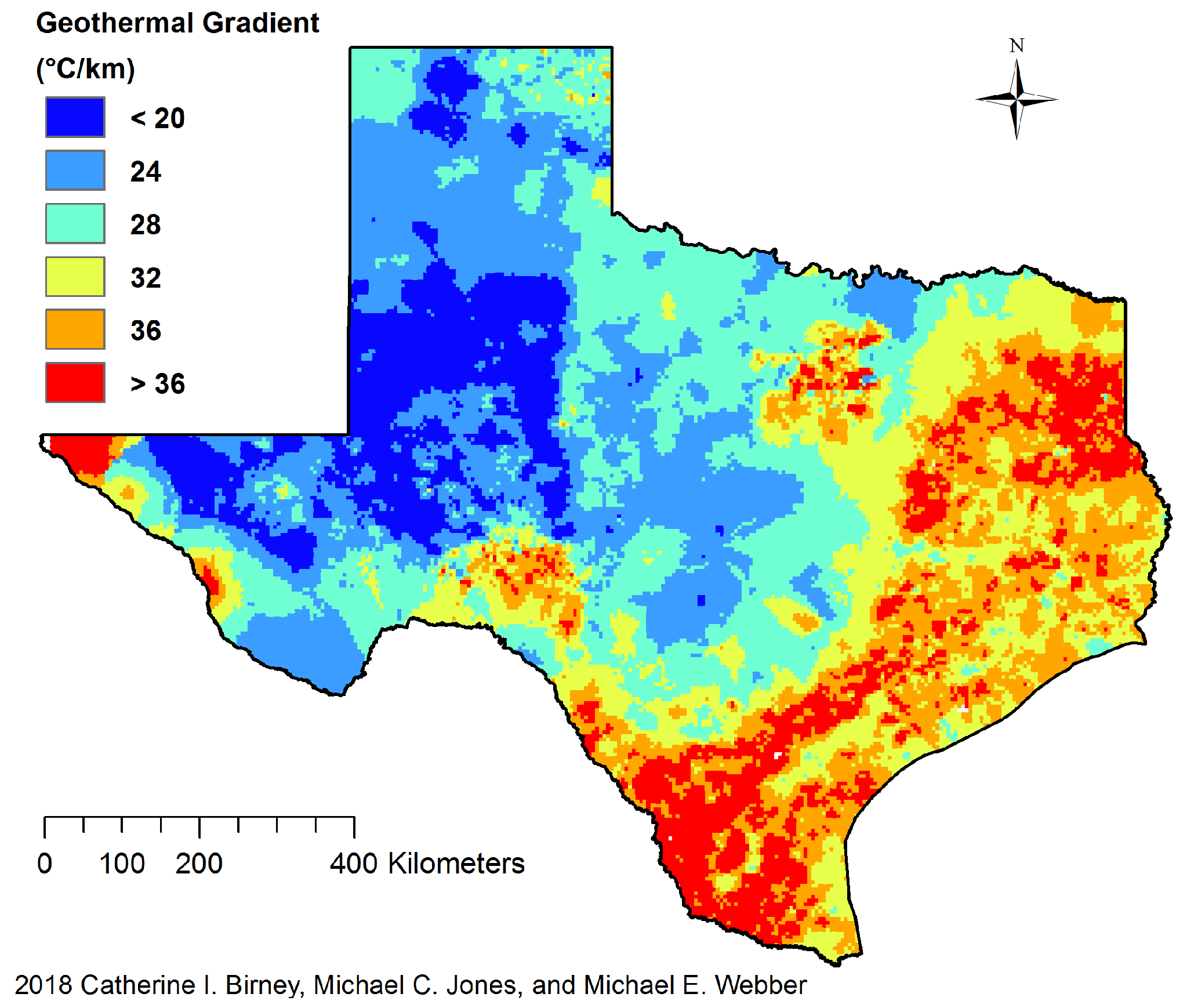
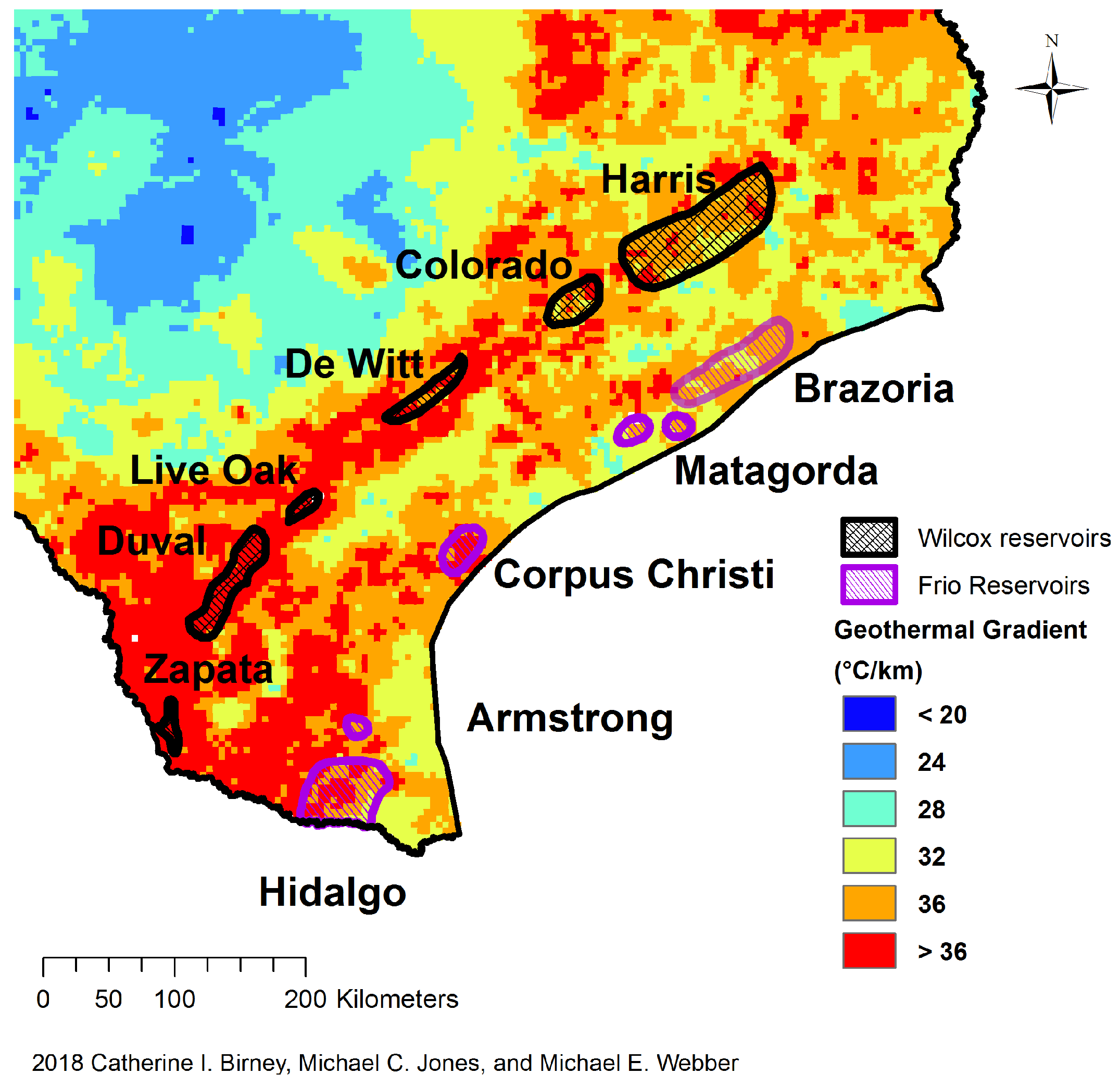
1.1. Texas as a Case Study

Texas is the focus of this case study because of anticipated water requirements and data availability. From 2010 to 2060, Texas’ existing water supplies are predicted to decrease by 10%, while the water demand increases by 22% [17]. Texas policy makers are searching for new freshwater sources to meet future water demands. Eight of the 16 water-planning regions in the state propose desalinating both brackish groundwater and seawater to meet future demands [17]. Texas has more than 2.7 billion acre-feet of brackish groundwater, water with a total dissolved solids (TDS) level between 1000 and 10,000 mg/L [17]. Texas currently has 46 brackish groundwater desalination plants capable of producing 170 million m3 per year. The State Water Plan, the main water-planning document for the state, recommends an additional 86 million m3 per year of groundwater to be desalinated in 2020 and 137 million m3 per year in 2070 to help meet water demands.
Texas has low-enthalpy geothermal resources with temperatures less than 150 ° C at depths of 3000–4000 m. Desalinating Texas’ brackish groundwater requires a design for low temperature resources. The framework of this study can be modified to other sites with low-enthalpy resources, but with varying geothermal gradients, salinity, and well depth.

1.2. Desalination Design

Desalination techniques can be categorized into two overarching approaches: Thermal processes and membrane processes. Thermal desalination techniques include multi-stage flash (MSF) distillation and multi-effect distillation (MED). Membrane processes include reverse osmosis (RO), nano-filtration, electro-dialysis (ED), and forward osmosis (FO). Membrane distillation (MD) combines principles of thermal and membrane processes. As this paper focuses on using geothermal resources, only thermal desalination techniques are considered for analysis.
MSF distillation is the process of desalinating water using a “flashing” system. The water is often less than 100 ° C, but when pressurized and released into a vacuum chamber, the water flashes into steam. The steam condenses into distilled water in a series of “effects” or “stages” with decreasing pressure. MED is similar to MSF, in that seawater or brackish water evaporates and condenses in a series of effects. The brackish water is sprayed into each effect, landing in a thin film on tubes filled with steam or hot water, causing evaporation [18].
The MED process has several advantages over MSF plants for low temperature heat resources. Namely, MED has lower energy consumption, higher heat transfer coefficients, and lower temperature drops between effects [19,20]. MED systems are optimized to have low top brine temperatures (TBT) ranging from 60–75 ° C, for better utilization of low grade heat sources [20,21]. The TBT is the maximum temperature the brine can reach in the MED system; temperatures above this range will cause scaling and corrosion [21,22]. Low-enthalpy geothermal sources have incoming temperatures up to 160 ° C, and to prevent silica scaling, the geothermal resources are rejected at temperatures between 60–80 ° C [23].
To power the desalination system, the geothermal water is also used to generated electricity, which can be accomplished through three methods [24]. The first is a dry steam power plant, best suited for steam resources. The second is a flash steam power plant, ideal for high pressure water at temperatures exceeding 182 ° C. The third is the binary cycle, which is best for water sources less than 182 ° C. As Texas has geothermal water sources less than 182 ° C at shallow depths, the binary cycle is ideally suited to be paired with the MED system. Combining MED with a binary cycle allows for the production of freshwater without the need for a grid connection under certain conditions.

1.3. Implementation of a Geothermal MED Plant

Cultures across the globe have used geothermal energy for bathing and space heating for centuries [25]. Geothermal generated electricity began in the early 1900’s, with the first commercial geothermal power plant built in 1913 [25]. The first conceptualized geothermal desalination unit was designed in 1976 [14]. The last several decades have seen an increasing interest in using geothermal energy for desalination and more specifically, to create self-powered systems [14,26].
There has been a successful implementation of a self-sufficient geothermal powered MED system. In 1999, a pilot geothermal MED plant was built on Kimolos Island, Greece [26]. The plant produced 75 m3 of water per hour, with a 61 ° C geothermal source. Using low-enthalpy geothermal energy, rather than energy purchased from the grid, prevented the consumption of 500 tonnes oil equivalent (TOE)/year [26]. Multiple studies have determined that geothermal heat sources of 100 ° C can be used to both generate electricity and desalinate water [14,25]. This research aims to use a spatial methodology to determine the best locations for implementing existing technology.

2. Materials and Methods

The analysis of a geothermal driven MED system, shown in Figure 1, to produce freshwater is comprised of three steps: (1) Using a thermodynamic model to estimate the potential of electricity production from a binary cycle to offset the electricity requirement of the system, (2) using a water treatment model to quantify the MED system’s rate of freshwater production based on the geothermal resource, and (3) using a multi-criterion geospatial analysis to estimate the geographic feasibility of implementing the combined system based on factors such as brackish groundwater depth, temperature, salinity, and flow rate. Both the binary cycle and the MED system are used to model Texas’ geothermal desalination potential due to the low-enthalpy resources available. The combined resource and spatial analysis provide a novel framework to assess possible geothermal desalination implementation. One of the most important factors is temperature, as the geothermal water resource must be hot enough to power both the binary cycle and the MED. The method is illustrated using Texas as a testbed because it has significant water challenges, its geothermal resources are abundant, and the data are available with high fidelity.
The thermodynamic and water treatment models are calculated using a spreadsheet analysis with geothermal data from Southern Methodist University and brackish groundwater data from the Texas Water Development Board [27,28]. The solver tool is used to optimize the electricity produced in the system, with an objective of minimizing the overall energy intensity. The model is constrained by thermodynamic properties and the number of possible effects in the MED system. Properties such as the geothermal flow rate, initial geothermal temperature, and efficiencies are varied to determine impacts on the system. The software ArcGIS is used to estimate output from the MED-binary cycle in a spatially-resolved way across Texas, using data from Southern Methodist University and the Department of Energy as inputs [27,29,30].

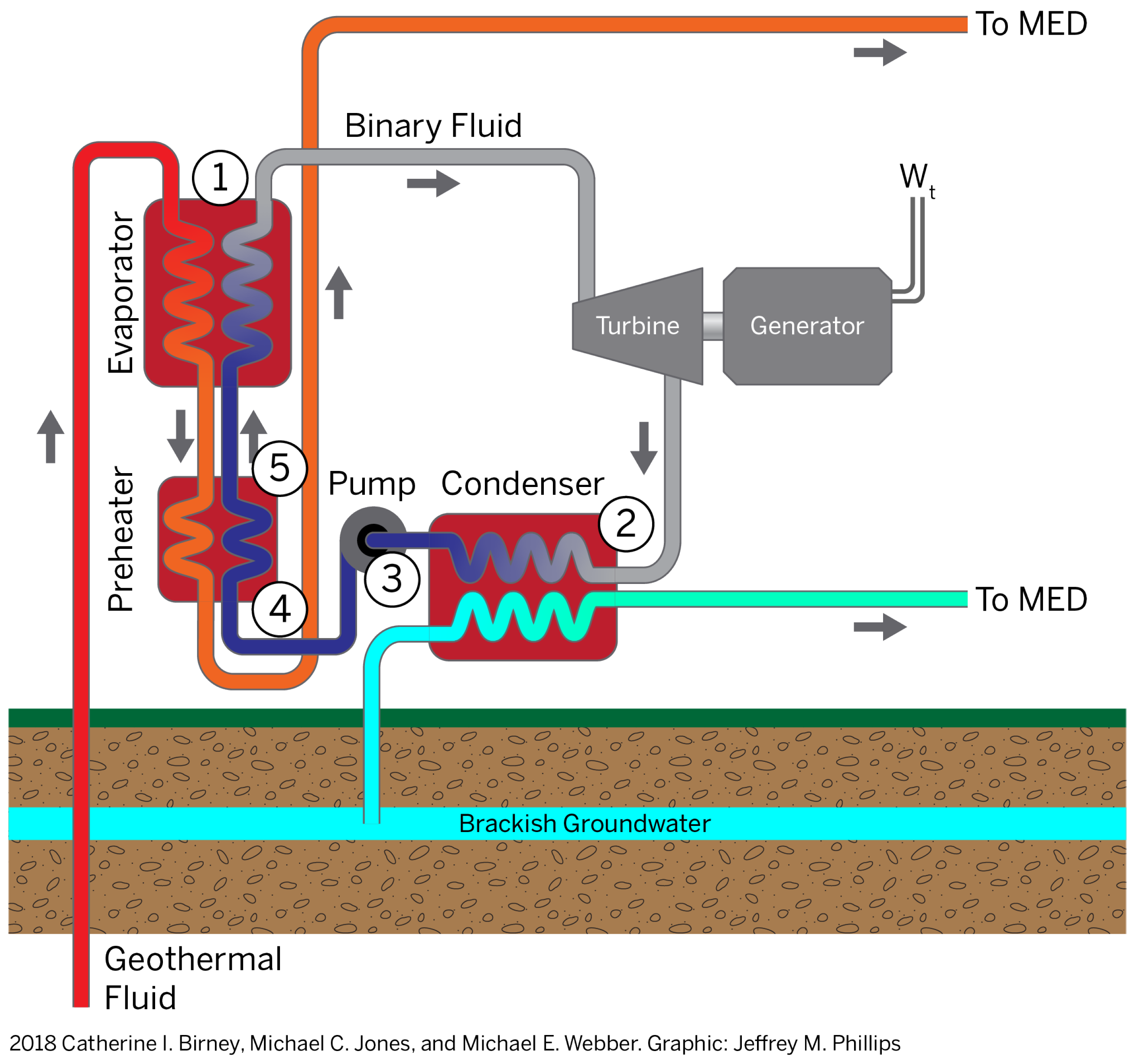
2.1. Principle of the Binary Cycle

Texas’ hottest geothermal resources at the shallowest depths occur mostly in southeast and east Texas, as illustrated in Figure 2. Texas’ resources are classified as low to moderate, as the majority of the resources are less than 150 ° C at depths of around 3000–4000 m.
Because Texas’ geothermal resources are mostly comprised of low-grade heat, a suitable method of producing electricity is using a closed loop Binary Organic Rankine Cycle, shown in Figure 3. Models for analyzing a geothermal binary cycle have been thoroughly developed and published in the literature as summarized below [31].
The hot geothermal fluid runs through a heat exchanger, at a predetermined flow rate, m g , with a specific heat capacity of c p , g dependent on the water temperature and salinity. Heat is transferred to a working fluid with a lower boiling temperature than water. Typical working fluids are hydrocarbons and synthetic refrigerants such as isobutene, isopentane, and R134a. This case study uses isopentane, one of the most common binary working fluids [32]. Equation (1) shows the thermodynamic relations used to assess the energy balance of the binary cycle system and to correlate the temperature change of the geothermal fluid to the incoming and outgoing enthalpy of the working fluid.
m ˙ g c p , g ( T g , 1 T g , 2 ) = m ˙ w f ( h 1 h 5 ) ,
where:
  • m ˙ g = Mass flow rate of geothermal water [kg/s].
  • c p , g = Specific heat capacity of geothermal water [kJ/kg-K].
  • T g , i = Temperature of the geothermal water at point i in Figure 3 [K].
  • m ˙ w f = Mass flow rate of working fluid in binary cycle [kg/s].
  • h i = Enthalpy of working fluid at point i in Figure 3 [kJ/kg].
The working fluid vaporizes in the evaporator then enters the turbine, rotating the blades and generating electricity, W t . The electricity generated is dependent upon the turbine efficiency, η t , the generator efficiency, η g , and the energy balance of the working fluid entering and exiting the turbine. It is assumed that there are no efficiency losses in the piping. Equation (2) is used to determine the electrical power W ˙ t generated by the binary cycle.
W ˙ t = m ˙ w f ( h 1 h 2 ) = m ˙ w f η t η g ( h 1 h 2 s ) ,
where:
  • W ˙ t = Rate of work output from turbine [kW].
  • η t = Turbine efficiency [%].
  • η g = Generator efficiency [%].
  • h 2 s = Isentropic enthalpy of working fluid at point i in Figure 3 [kJ/kg].
After generating power in the turbine, the working fluid enters the condenser, where it is cooled and condensed by the brackish groundwater flowing to the MED system to be desalinated. Using the brackish groundwater as the coolant accrues two benefits: (1) The brackish water is preheated, which improves throughput in the MED, and (2) the binary cycle is cooled, improving its efficiency, in a way that does not require any freshwater. A binary plant can have either a wet cooling system or a dry cooling system. A wet system condenses the working fluid using cooling water, while the dry system uses air cooling. As the ambient air temperature in Texas is high, 40–50% of the energy produced by the binary cycle would go to cooling the system [23]. Therefore, a wet cooling system is better suited for Texas’ climate, though it could exacerbate water scarcity issues.
As there is minimal increase in the feed water temperature after preheating, the specific heat of the feed water, c p , f , is assumed constant. Equation (3) shows the thermodynamic relations between the feed water and the working fluid and is used to determine the final temperature of the brackish feed water before the water flows into the MED system for desalination.
m ˙ f c p , f ( T f , 3 T f , 2 ) = m ˙ w f ( h 2 h 3 ) ,
where:
  • m ˙ f = Mass flow rate of feed water (brackish groundwater) [kg/s].
  • c p , f = Specific heat capacity of feed water [kJ/kg-K].
  • T f , i = Temperature of feed water at point i in Figure 3 [K].
The pump, W ˙ p , continues to circulate the cooled working fluid, consuming a portion of the power generated by the turbine. The energy requirements for pumping are based on the efficiency of the pump, η p . Equation (4) is used to calculate the power required by the pump.
W ˙ p = m ˙ w f ( h 4 h 3 ) = m ˙ w f ( h 4 s h 3 ) η p ,
where:
  • W ˙ p = Rate of work required by binary cycle pump [kW].
  • η p = Pump efficiency [%].
The working fluid enters the preheater, where the fluid is heated by the geothermal water, ensuring that the working fluid will vaporize in the evaporator and rotate the turbine blades. Equation (5) is used to determine the temperature change in the geothermal water and working fluid.
m ˙ g c p , g ( T g , 2 T g , 3 ) = m ˙ w f ( h 5 h 4 ) .
The process repeats in this closed loop binary cycle. The efficiency of the binary cycle, η t h , is generally between 5–15% and is analyzed using Equation (6) [23,31]. W ˙ n e t is the net work generated by the turbine and Q ˙ P H / E is the heat exchanged from the geothermal fluid to the working fluid in the pre-heater and the heat exchanger.
η t h = W ˙ n e t Q ˙ P H / E = 1 h 2 h 3 h 1 h 4 .
The purpose of using the geothermal water to generate electricity before providing heat to the MED system is to offset or eliminate the electricity requirements for running the system. Meeting the electricity requirements completely would enable this system to run autonomously. To compare electricity generation to consumption, the energy requirements for pumping the geothermal fluid, P p , g , and brackish groundwater, P p , f and the energy requirement for the desalination process, P D , in the MED plant is considered. Equation (7) represents the total power required to run the binary-cycle MED plant.
P = P p , g + P p , f + P D .
The energy requirements for pumping the geothermal and brackish groundwater are determined from Equation (8). The pumping requirements are based on depth to source water, Z i , pump efficiency, η p , and the capacity factor of the system, C F D , assumed to be 95% for this analysis. The energy requirements for the system can be drastically reduced if the geothermal water is from a geopressured reservoir, where the water flows freely to the surface and does not need to be pumped.
P p , i = ρ g q i 1000 η p C F D × [ Z i + ( 4 q i π d 2 ) 2 2 g × f d × ( Z i + l ) ] ,
where:
  • ρ = water density (kg/m3).
  • g = acceleration due to gravity (m/s2).
  • q i = volumetric flow rate of water (m3/s).
  • η p = pump efficiency (%).
  • C F D = desalination capacity factor.
  • Z i = depth to water (m).
  • d = pipe diameter (m).
  • f = friction factor.
  • l = pipe length (m).
The remaining energy requirement is the energy required for the desalination process, which is calculated using Equation (9). The energy for desalination is based off the capacity factor, C F D , the energy intensity, E D (kwh/m3), and the volumetric flow rate of the brackish feed water, q f .
P D = E D × q f C F D .

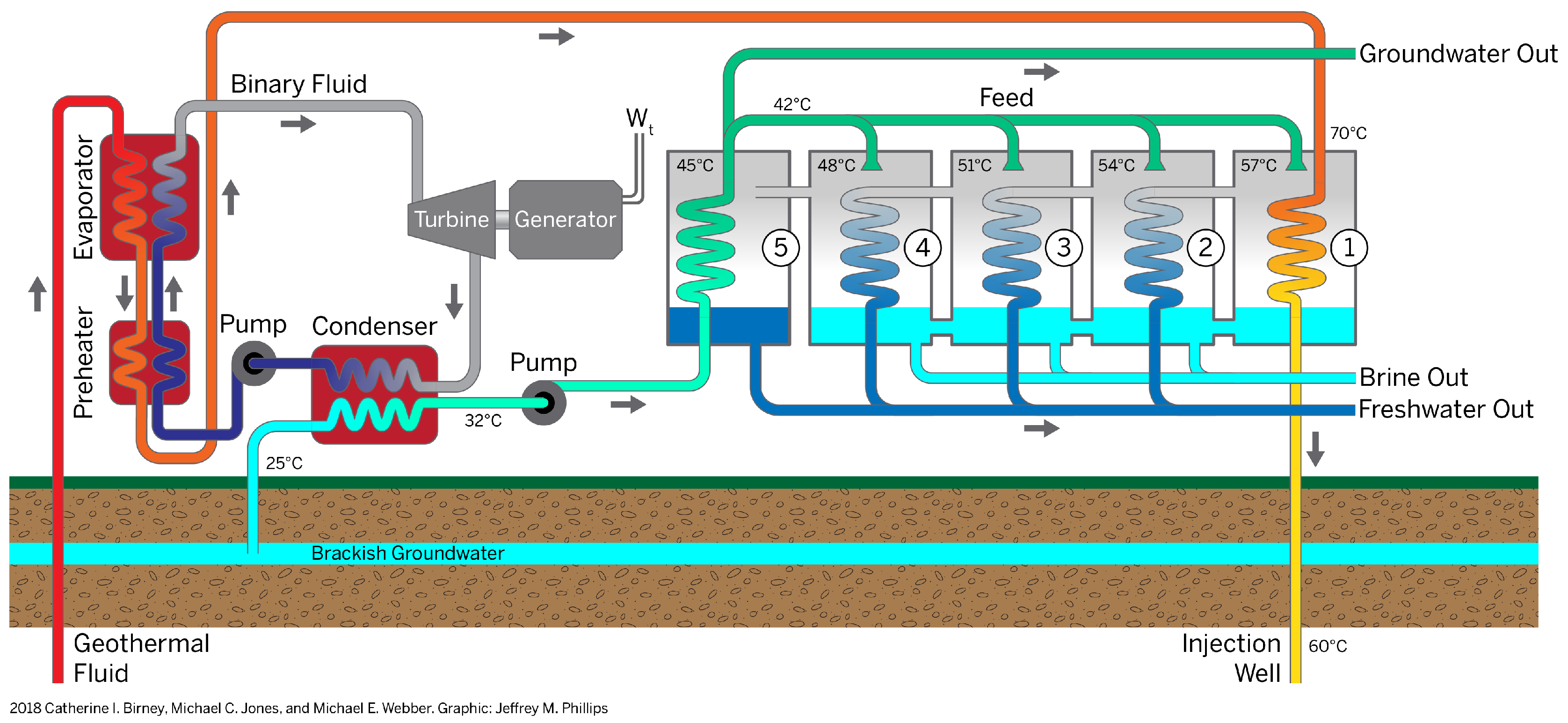
2.2. Principle of the Multi-Effect Distillation System

Both the geothermal fluid and the feed water enter the MED system after moving through the binary cycle, as shown in Figure 1. The MED system uses a series of evaporator effects with decreasing pressure to desalinate water. The geothermal water enters the first effect as the heat source for the entire system. The geothermal water is kept in a closed loop and upon exiting the first effect, is returned to the original groundwater source via an injection well.
The pressure in the first effect is set relative to the incoming geothermal heat source and is used to evaporate the incoming feed water (brackish groundwater). The feed water first enters the condenser as the cooling source for the vapor leaving the final effect. The feed water is sprayed into each effect, whereupon the water vaporizes and enters the subsequent effect as the heat source to evaporate the entering feed. The pressure in the second effect is set lower than that of the first effect to decrease the boiling point temperature. The pressure is lowered in each subsequent effect. The MED system concludes with a condenser, where the steam from the last effect enters and is condensed via the feed water. The condensed steam exits as freshwater. Any feed water that does not evaporate collects and exits through the bottom of each effect as brine, a highly concentrated saline solution, which requires disposal or separate treatment, adding to the cost of desalination. The numerical model for the MED system is adapted from the literature [22,33]. The model is analyzed in three components for a system with n effects: The first effect, effects 2 through n 2-n, and the condenser.
The energy balance for the first effect, the nth effect, and the condenser are shown in Equations (10)–(12), respectfully. The equations are solved for m ˙ n , v , the mass flow rate of the vapor created in each effect.
Q 1 ˙ = m ˙ g c p , g ( T 1 , g , i n T 1 , g , o u t ) = m ˙ 1 , f c p , f ( T 1 , b T 1 , f ) + m ˙ 1 , v h 1 , f g ,
Q ˙ n = m ˙ n 1 [ c p , v ( T n 1 , b T n , v s ) + h n 1 , f g ] = m ˙ n , f c p , f ( T n , b T n , f ) + m ˙ n , v h n , f g ,
Q ˙ z = m ˙ z 1 , v [ c p , v ( T z 1 , b T z , v s ) + h z 1 , f g ] = m ˙ z c p , z ( T z , o u t T z , i n ) ,
where:
  • T 1 , g , i n = Geothermal temperature entering 1st effect in Figure 1 (K).
  • T 1 , g , o u t = Geothermal temperature exiting 1st effect in Figure 1 (K).
  • m ˙ n , f = Mass flow rate of feed water entering effect n in Figure 1 (kg/s).
  • T n , b = Temperature of brine exiting effect n in Figure 1 (K).
  • T n , f = Temperature of feed water entering effect n in Figure 1 (K).
  • m ˙ n , v = Mass flow rate of vapor in effect n (kg/s).
  • h n , f g = Latent heat of evaporation in effect n (kJ/kg).
  • c p , v = Specific heat of water vapor (kJ/kg).
  • T n , v s = Vapor saturation temperature, effect n (K).
The latent heat of evaporation, h f g , is dependent on the boiling temperature of each evaporator, and can be calculated from the vapor saturation temperature, T v s , which in turn can be calculated from the boiling temperature T b of each effect [22,33]. These relationships are shown in Equations (13) and (14).
h f g = 2494.57 2.20486 T v s 1.596 × 10 3 T v s 2 ,
T v s = T b B P E .
The Boiling Point Elevation ( B P E ) calculated in kelvin and shown in Equation (14), is the increase in the boiling temperature due to the salts in the water. The B P E can be calculated based on the salt concentration, S, and boiling temperature, T b , as shown in Equation (15) [22,33].
B P E = A S 2 + B S , A = 4.584 × 10 4 T b 2 + 2.823 × 10 1 + 17.95 , B = 1.536 × 10 4 T b 2 + 5.267 × 10 2 T b + 6.56 .
The freshwater generated from the MED system is the sum of the vapor from each effect and is calculated in Equation (16).
m ˙ f w a t e r = i = 1 z m ˙ n , v .
The MED system faces certain constraints. Water production is limited by the recovery factor. The recovery factor is the ratio of the mass flow rate of the feed to the mass flow rate of the recovered freshwater. The recovery factor is set to 1.8 in this analysis, a similar value to those in the literature [21].
Additionally, the MED system is limited by pinch point temperature and TBT. The pinch point is the minimum temperature difference between the brine and the geothermal water in the heat exchanger in the first effect [31], represented by Equation (17). The pinch point temperature is set to 5 ° C in this analysis, a number found in the literature [13]. The MED system is also limited by the TBT, as previously discussed, and is set to 70 ° C.
T 1 , 1 , p p = T 1 , 1 , i n m ˙ 1 , v h f g , 1 , 2 m ˙ g c p , g + T H E ,
where:
  • T H E = Temperature difference between liquids in the heat exchanger in the first effect [K].

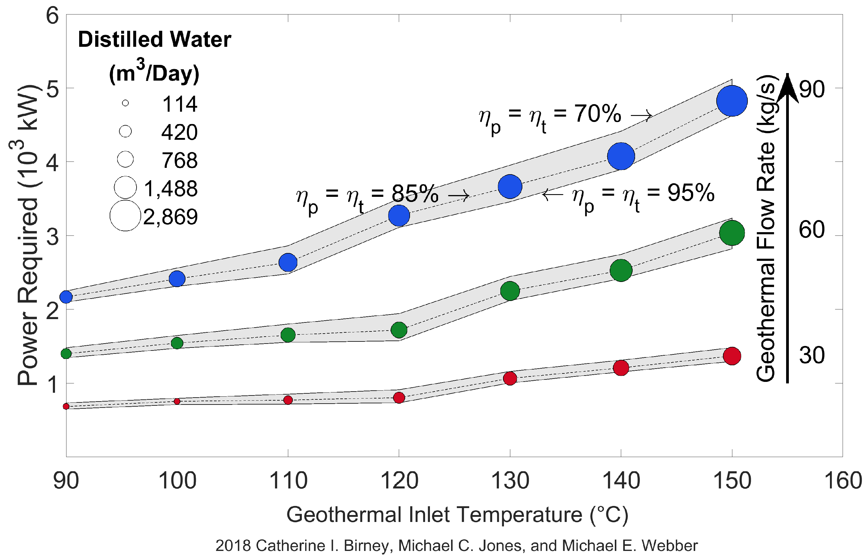
2.3. Resource Feasibility in Texas for Binary-MED System
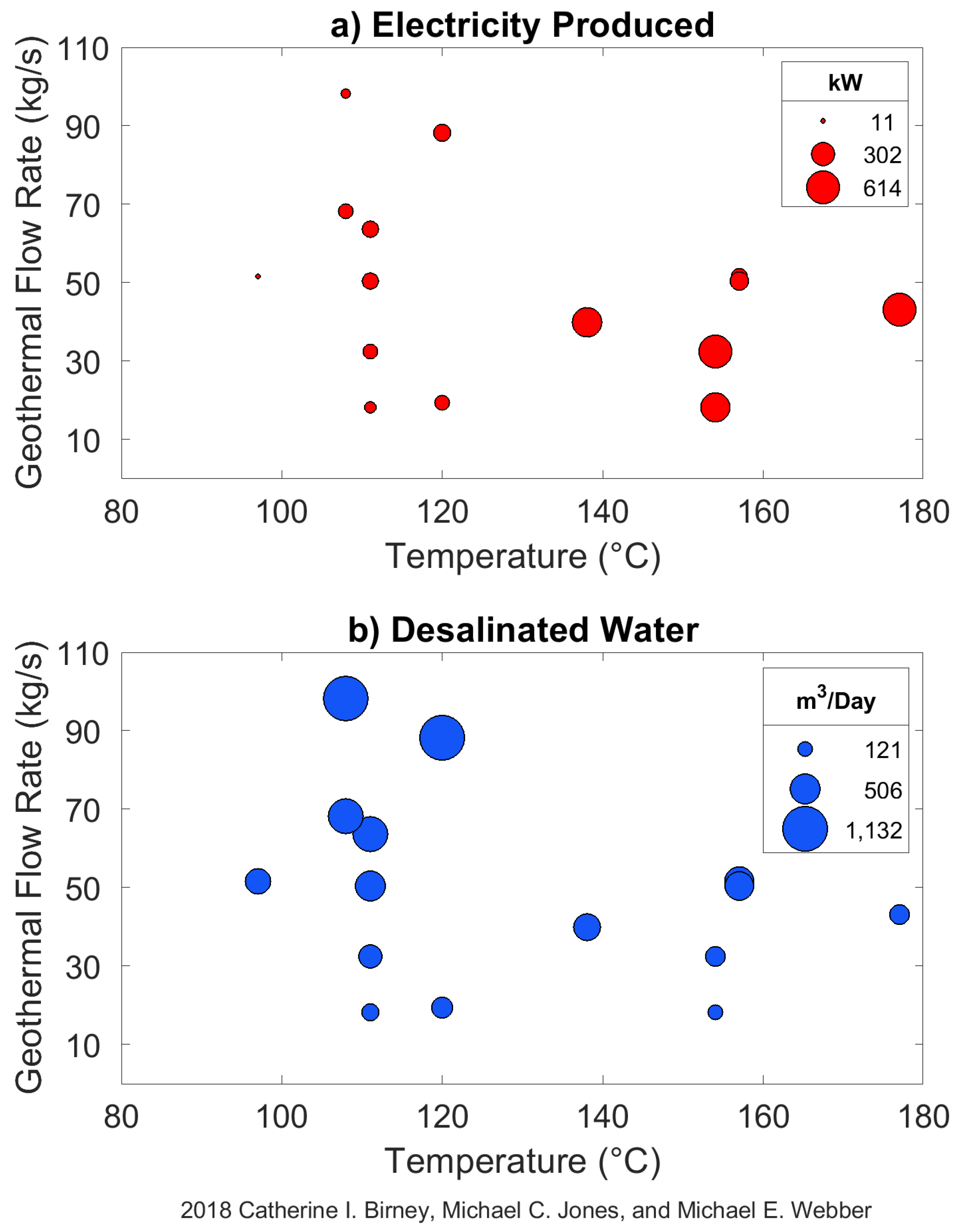
A desirable location for the Binary-MED system will have hot geothermal resources at a shallow depth in a geopressured zone, as the water in that case would not require pumping to the surface. A desirable location will also have an abundant brackish groundwater resource with low salinity at a shallow depth. As the salinity of the water increases, the quantity of distilled water decreases and the quantity of brine increases [34,35]. Geothermal resources in geopressured environments are uniquely suited to Binary-MED application, as the water is self-flowing and does not require a pump. In the 1970s the Department of Energy conducted a study on Texas’ geothermal resources, including an assessment of pressure and flowrate information, and determined promising geopressured zones [29,30]. These geopressured zones line up with some of Texas’ hottest resources, in East Texas and along the Gulf Coastal Plain. In addition, these regions are littered with abandoned oil and gas wells, which can be utilized for geothermal desalination. In April 2017, there were over 100,000 inactive wells, which are wells that are unplugged and unproductive for over a year [36]. Utilizing existing wells can reduce or eliminate the cost of drilling.
Geopressured geothermal resources vary from conventional hydrothermal-geothermal systems in both energy source and content. Conventional geothermal heat is generated by various processes associated with tectonic forces, illustrated by the abundance of geothermal sites located along the Pacific Ring of Fire. Unlike the igneous and metamorphic environments most commonly associated with conventional geothermal resources, geopressured geothermal resources are unique to sedimentary systems. These systems are characterized by abnormally high pore pressure gradients, which describe the pressure values within the fluid filled pores of sedimentary rock sections as a function of depth. A common mechanism responsible for producing geopressured conditions is compaction disequilibrium [37]. Under normal circumstances, sediments are compacted when subjected to stress. As compaction occurs, water is expelled and pore pressure remains constant. If low permeability sediment impedes fluid flow, pressure builds as a function of the weight of the overlying sediment. Since heat and pressure at a constant volume are proportional, heat is concentrated within geopressured sediments. A conceptual model of geopressured reservoirs is shown in Figure 4.
As opposed to conventional hydrothermal resources, which contain usable energy only in the form of heat, geopressured resources have usable energy in three forms: Mechanical energy via highly pressurized reservoir fluid, thermal energy in the form of the heated reservoir fluid, and chemical energy in the form of co-produced methane found within the reservoirs. This work only examines the first two forms of energy, though methane co-production might significantly improve the energy balance and cost-effectiveness of the approach described in this manuscript.
Areas of exploitable geopressured resources are located in the geologic environment known as the Tertiary Gulf Coast Depositional Wedge [38]. This sedimentary section is prominently made up of gulfward thickening layers of alternating sand and shale. In their more southeast/gulfward extents (i.e., downdip), these layers drastically thicken due to the development of growth faults. These faults develop as deposition occurs and are a product of denser sands deposited on loosely-packed shale. This process of growth faulting commonly results in the expansion of the downthrown sediment. Repeated faulting and expansion leads to the development of large, vertically expansive geopressured sand reservoirs. This general reservoir structure is shown in Figure 5.
A viable geothermal resource is generally characterized by expansive reservoir volumes, presence of a mobile reservoir fluid, and adequate reservoir temperature at economically reachable depths. Viable expanded geopressured reservoirs are predominantly found in two growth faulted geologic sections along the Texas gulf coast: The Frio Formation and Wilcox Group. Geopressured conditions also exist in more inland regions of East Texas near the Sabine Uplift, but are limited to dry gas reservoirs created in slope and basin floor environments (see Figure 5). Other high temperature geopressured resources are found along the gulf coast and in East Texas but are not as vertically expansive and often do not contain a mobile fluid required for energy production.
A geospatial distribution model was created to quantitatively determine the most suitable locations for a theoretical geopressured geothermal energy production system known as a well bore heat exchanger [40]. Bottom hole temperature data from 42,601 wells are displayed in Figure 6.
Using ArcMap Analysis and Spatial Statistics tools, areas with a large number of oil and gas wells with high bore hole temperature (BHT) were defined. The Cluster and Outlier Analysis tool solves for the Anselin Local Moran’s I statistic of spatial association, shown in Equation (18).
I i = x i X ¯ S i 2 j = 1 , j 1 n w i , j ( x i X ¯ ) ,
where I i is the statistic of spatial association, X i is bottom hole temperature, X ¯ is the mean bottom hole temperature, w i , j is a predetermined spatial weight between wells, n is the number of wells, and S i 2 is calculated using Equation (19).
S i 2 = j = 1 , j 1 n w i , j n 1 X ¯ 2 .
This calculated value ( I i ) was used to display concentrations of wells with high bottom hole temperatures. To display the results in a meaningful map view, multiple iterations of this calculation were executed with different lower bounds or “floors” to the bottom hole temperature data set. The resulting outputs, when stacked in order of higher floor bounds overlying lower floor bounds, created a “composite cluster overlay,” displaying a heat-map-like pattern showing discrete clusters of increasing temperature attribute values. Temperature values of each increasing floor increment were based on an equal interval classification scheme containing 10 classes as displayed on the histogram in Figure 7.
Altering the method of classification and number of classes allows for varying outputs based on a desired composite cluster resolution or an altered emphasis from the attribute values to the features themselves. For example, using the quantile method of classification would ensure an equal number of features per class. This method considers an escalating floor that removes an equal number of wells in each iteration. Final results of this composite cluster analysis are displayed geographically by a 1.6-km (1-mile) buffer around the clustered features. This arbitrary buffer distance was chosen to allow for interpretation of clustering on both a state wide and local basis. Figure 8 shows a view of three areas containing high attribute value clusters.

3. Results

The methods for assessing electricity, water production, and geothermal resource quality discussed in Section 2 are used together to determine the potential of implementing a self-sufficient desalination system in Texas. The overall geothermal binary-MED system is modeled for areas of Texas with a geothermal gradient of 36 ° C/km. This temperature gradient represents the lower end of Texas’ hottest geothermal resources, as shown in Figure 2. The water is pumped from depths ranging from 1800–3500 m, with temperatures ranging from 90–150 ° C. Assumptions made for these calculations are shown below in Table 1. Pumping water from these depths is energy-intensive, making it difficult for the binary-MED system to reach standalone energy self-reliance. Figure 9 shows the model results for scenarios with varying geothermal flow rates and temperatures. In all of the proposed situations, the binary cycle is unable to produce all the power required to pump the water from such depths, but does distill 114–2869 m3 of water per day. For an average person’s use of 0.5 m3/day, this system can provide water for 214–5400 people per well.
The simulations in Figure 9 show that as flow rate is increased, the production of freshwater increases, which is consistent with MED operation. For an incoming geothermal temperature of 120 ° C, the freshwater production increases from 386 m3 per day, to 768 and finally 1367 m3 per day as the flow rate increases from 30 to 60 to 90 kg/s, respectively. As more water is pumped from the ground, more heat can be transferred to the working fluid in the binary cycle and then to the brackish groundwater in the MED system. Geothermal temperatures of 90–110 ° C are not hot enough to fully power both the binary cycle and the MED system. At temperatures this low, there is a trade-off between producing electricity and producing freshwater. As this system’s primary notional purpose is to produce freshwater rather than electricity, a boundary condition is imposed on the geothermal water exiting the binary cycle, preventing the water temperature from dropping below 70 ° C. The boundary condition results in less heat being transferred out of the geothermal resource than would be possible if the system were optimized to produce electricity, so the binary cycle does not run at its optimum efficiency. Figure 9 also shows that the hotter the geothermal resource, the more water that can be distilled. However, pumping from greater depths to access hotter geothermal resources results in an increase in the electricity requirement because pumping water is so energy intensive.
Due to the high energy requirements of pumping water, the best location for a self-sufficient binary-MED plant is in a geopressured region. The results of the composite cluster analysis described in Section 2.3 verify the previous outline of geothermal regions defined by the Department of Energy 1970 study [29], which separated the Wilcox and Frio formations into individual fairways as shown in Figure 10. As these zones are geopressured, the water is self flowing and does not need to be pumped, eliminating a large portion of the MED energy load.
Studies conducted on the fairways identified flow rates and temperatures of wells within the zones. Figure 11 shows potential results that can be found in some areas of the fairways. The results are promising in these zones, as both freshwater and electricity can be produced. The results find that 121–1132 m3 of water per day can be desalinated, enough water for 232–2133 people. At the same time, some of these zones could produce an excess of electricity, with the sample wells analyzed with this work producing 11–614 kW. To produce more water and more electricity, multiple wells can be utilized in the same area. These results were found using the thermodynamic model integrated with the GIS map of Texas, using data from SMU and the DOE [27,30].

4. Discussion

As population increases and freshwater resources become scarcer, water planners and decision makers are looking for new sources of water. Coupling a low carbon energy source, such as geothermal energy, with an energy-intensive water treatment system, such as desalination, is a method of producing drinking water without exacerbating carbon emissions.
This study uses an integrated thermodynamic and GIS model of Texas’ geothermal and brackish groundwater resources to conduct a geographical assessment for the potential implementation of a geothermal powered MED plant. We model multiple scenarios, testing the viability of on-site geothermal electricity generation to power the desalination process, while optimizing fresh water production. Water production is maximized based on well depth, total dissolved solids concentration of the brackish water, and temperature of the water source.
This analysis finds that in the geopressured Frio and Wilcox fairways located in southeast Texas, a geothermal powered MED plant could be built to run self-sufficiently, without the need for electricity from the grid. Wells in these fairways could produce 121–1132 m3/day of freshwater, enough to supply 232–2133 people. An additional benefit is that there are over 100,000 inactive and unplugged oil and gas wells in these regions. Utilizing existing wells can reduce or eliminate the cost of drilling associated with geothermal power production. In all other locations of Texas, a geothermal powered MED system would have to purchase additional electricity from the grid or be built in conjunction with a second renewable energy source, such as solar or wind.
Without the unplugged wells littered across the fairways, it is unlikely that geothermal powered desalination would be economically feasible in Texas. As noted by other studies, geothermal desalination is only cost-effective with access to cheap geothermal reservoirs, but does hold the advantage of being a steady heat source over other renewable energy sources [13,41,42].
This system could run completely on renewable energy and independently of the grid in non-geopressured regions if paired with an additional renewable energy source, such as wind or solar [7,8]. MED has an advantage over membrane desalination processes, as ramping thermal desalination up and down does not cause damage to the internal parts of the desalination system [43]. Paired with wind or solar energy, the system could be programmed to run only when the wind and/or solar energy is providing enough of an additional energy input to fully power the desalination process.
Our assessment found that the most important factors in determining if a geothermal powered MED system can operate self-sufficiently is the geothermal temperature and depth to water. The salinity of the groundwater has little impact on brackish groundwater desalination using an MED system. These conclusions are similar to a study by Loutatidou, who conducted a sensitivity analysis and found that depth, well productivity, and temperature are impactful on the desalination outcome, while salinity and seawater feed temperature are less important [13].
The assessment of Texas’ geothermal energy sources for desalination adds to the literature focused on co-locating renewable energy with desalination plants [7,8]. The results find that different methods of renewable energy work well in different areas of Texas. Solar powered desalination is ideal for Northwest Texas, combined solar and wind systems work well in Central Texas and geothermal energy can power systems in Southeast Texas. Renewable powered desalination systems must be designed based on the available resources.
Beyond being beneficial for Texas water planners, this research provides a framework for assessing viable locations for geothermal powered desalination facilities. This methodology is scalable and can be modified to individual aquifer or national level analyses, depending on the needs of the planner. Geothermal has significant potential as an energy source, even at the low temperatures found in Texas. It is a baseload power source that can continuously produce electricity without incurring fuel costs. Geothermal energy is free from greenhouse gas emissions at the point of generation, an important factor to consider when determining the future of energy in the United States and the world.

Limitations and Future Work

Two limitations of this research are that the study does not address the environmental concerns of brine disposal and the research does not address the economic components of building a geothermal MED plant. Both of these issues are out of scope of this project, as the research goal was to develop a spatial framework for assessing geothermal resources. Thorough economic analysis can be found in the literature [6,13,44].
Future work should include an economic analysis specific to building a geothermal powered MED plant in the Frio and Wilcox fairways, accounting for use of unplugged wells. This type of analysis would be helpful and necessary for policymakers. Additional work could explore combining geothermal energy with other renewable energy sources, such as wind and solar. Wind and solar powered desalination potential have been assessed separately for Texas [7,8].
The results of this study can be improved by considering alternative working fluids for the binary cycle. In this paper, isopentane was selected as the working fluid, however mixing isopentane with isobutene might lead to better results, as mixtures have some advantages over pure compounds [45]. The energy production of the system could be improved by capturing the hydraulic energy in geopressured zones as the water flows up through the pipe. Additionally, in many geopressured zones, natural gas is an abundant resource, which can be captured to generate additional power and revenues.

Author Contributions

Conceptualization, C.I.B., M.C.J. and M.E.W.; methodology, C.I.B. and M.C.J.; software, C.I.B. and M.C.J.; validation, C.I.B.; formal analysis, C.I.B. and M.C.J.; investigation, C.I.B. and M.C.J.; resources, M.E.W.; data curation, C.I.B. and M.C.J.; writing—original draft preparation, C.I.B. and M.C.J.; writing—review and editing, C.I.B. and M.E.W.; visualization, C.I.B.; supervision, M.E.W.; project administration, C.I.B.; funding acquisition, C.I.B. and M.E.W.

Funding

This research was funded by the National Science Foundation (NSF) Graduate Research Fellowship Program (GRFP) and the Cynthia and George Mitchell Foundation.

Conflicts of Interest

The authors declare no conflict of interest. The funders had no role in the design of the study; in the collection, analyses, or interpretation of data; in the writing of the manuscript, or in the decision to publish the results.

Nomenclature

ParameterDefinitionUnit
c p , f Specific heat capacity of feed water(kJ/kg-K)
c p , g Specific heat capacity of geothermal water(kJ/kg-K)
c p , v Specific heat of water vapor(kJ/kg)
C F D Desalination capacity factor(%)
dPipe diameter(m)
E D Energy intensity(kwh/m3)
fFriction factor
gAcceleration due to gravity(m/s2)
h i Enthalpy of working fluid at point i in Figure 3(kJ/kg)
h i s Isentropic enthalpy of working fluid at point i in Figure 3(kJ/kg)
h n , f g Latent heat of evaporation in effect n(kJ/kg)
lPipe length(m)
m ˙ f Mass flow rate of feed water (brackish groundwater)(kg/s)
m ˙ g Mass flow rate of geothermal water(kg/s)
m ˙ n , f Mass flow rate of feed water entering effect n in Figure 1(kg/s)
m ˙ n , v Mass flow rate of vapor in effect n(kg/s)
m ˙ w f Mass flow rate of working fluid in binary cycle(kg/s)
η g Generator efficiency(%)
η p Pump efficiency(%)
η t Turbine efficiency(%)
η t h Binary cycle efficiency(%)
PPower to run binary-MED plant(kW)
P D Power requirement for the desalination process(kW)
P p , g Power requirements for pumping the geothermal fluid(kW)
P p , f Power requirements for pumping the brackish groundwater(kW)
ρ Water density(kg/m3)
q i Volumetric flow rate of water(m3/s)
Q ˙ P H / E Rate of heat transfer in heat exchanger(kW)
T 1 , 1 , p p Pinch Point Temperature(K)
T 1 , g , i n Geothermal temperature entering 1st effect in Figure 1(K)
T 1 , g , o u t Geothermal temperature exiting 1st effect in Figure 1(K)
T f , i Temperature of feed water at point i in Figure 3(K)
T g , i Temperature of geothermal water at point i in Figure 3(K)
T H E Temperature difference between liquids in the heat exchanger in the first effect(K)
T n , b Temperature of brine exiting effect n in Figure 1(K)
T n , f Temperature of feed water entering effect n in Figure 1(K)
T n , v s Vapor saturation temperature, effect n(K)
W ˙ n e t Rate of work generated by turbine(kW)
W ˙ p Rate of work required by binary cycle pump(kW)
W ˙ t Rate of work output from turbine(kW)
Z i Depth to water(m)

References

  1. UNEP. Vital Water Graphics-An Overview of the State of the World’s Fresh and Marine Waters; Technical Report; United Nations Environment Programme: Nairobi, Kenya, 2002. [Google Scholar]
  2. Varis, O.; Vakkilainen, P. China’s 8 challenges to water resources management in the first quarter of the 21st century. Geomorphology 2001, 41, 93–104. [Google Scholar] [CrossRef]
  3. Roudi-Fahimi, F.; Creel, L.; De Souza, R.M. Finding the Balance: Population and Water Scarcity in the Middle East and North Africa. Popul. Ref. Bureau 2002, 1, 1–8. [Google Scholar]
  4. UN-Water. Coping with Water Scarcity; Technical Report; FAO Water Reports: Chhattisgarh, India, 2006. [Google Scholar]
  5. Voutchkov, N. Desalination Engineering Planning and Design; McGraw-Hill Publishing: New York, NY, USA, 2013. [Google Scholar]
  6. Karagiannis, I.C.; Soldatos, P.G. Water desalination cost literature: Review and assessment. Desalination 2008, 223, 448–456. [Google Scholar] [CrossRef]
  7. Kjellsson, J.; Webber, M. The Energy-Water Nexus: Spatially-Resolved Analysis of the Potential for Desalinating Brackish Groundwater by Use of Solar Energy. Resources 2015, 4, 476–489. [Google Scholar] [CrossRef] [Green Version]
  8. Gold, G.; Webber, M. The Energy-Water Nexus: An Analysis and Comparison of Various Configurations Integrating Desalination with Renewable Power. Resources 2015, 4, 227–276. [Google Scholar] [CrossRef]
  9. Gude, V.G. Desalination and sustainability–An appraisal and current perspective. Water Resour. 2016, 89, 87–106. [Google Scholar] [CrossRef] [PubMed]
  10. McMorrow, D. Enhanced Geothermal Systems; Technical Report; The MITRE Corporation: McLean, VA, USA, 2013. [Google Scholar]
  11. Zafar, S.D.; Cutright, B.L. Texas’ geothermal resource base: A raster-integration method for estimating in-place geothermal-energy resources using ArcGIS. Geothermics 2014, 50, 148–154. [Google Scholar] [CrossRef]
  12. Tester, J.W.; Anderson, B.J.; Batchelor, A.S.; Blackwell, D.D.; DiPippo, R.; Drake, E.M.; Garnish, J.; Livesay, B.; Moore, M.C.; Nichols, K.; et al. The Future of Geothermal Energy-Impact of Enhanced Geothermal Systems (EGS) on the United States in the 21st Century; Technical Report; Massachusetts Institute of Technology: Boston, MA, USA, 2006. [Google Scholar]
  13. Loutatidou, S.; Arafat, H.A. Techno-economic analysis of MED and RO desalination powered by low-enthalpy geothermal energy. Desalination 2015, 365, 277–292. [Google Scholar] [CrossRef]
  14. Davies, P.A.; Orfi, J. Self-powered desalination of geothermal saline groundwater: Technical feasibility. Water 2014, 6, 3409–3432. [Google Scholar] [CrossRef]
  15. Spang, E. The Potential for Wind-Powered Desalination in Water-Scarce Countries. Ph.D. Thesis, Tufts University, Medford, MA, USA, 2006. [Google Scholar] [CrossRef]
  16. Grubert, E.A.; Stillwell, A.S.; Webber, M.E. Where does solar-aided seawater desalination make sense? A method for identifying sustainable sites. Desalination 2014, 339, 10–17. [Google Scholar] [CrossRef] [Green Version]
  17. Texas Water Development Board. 2017 State Water Plan; Technical Report; Texas Water Development Board: Austin, TX, USA, 19 May 2016.
  18. Raluy, G.; Serra, L.; Uche, J. Life cycle assessment of MSF, MED and RO desalination technologies. Energy 2006, 31, 2025–2036. [Google Scholar] [CrossRef]
  19. Shatat, M.; Riffat, S.B. Water desalination technologies utilizing conventional and renewable energy sources. Int. J. Low Carbon Technol. 2014, 9, 1–19. [Google Scholar] [CrossRef]
  20. Ophir, A.; Lokiec, F. Advanced MED process for most economical sea water desalination. Desalination 2005, 182, 187–198. [Google Scholar] [CrossRef]
  21. Rahimi, B.; Christ, A.; Regenauer-Lieb, K.; Chua, H.T. A novel process for low grade heat driven desalination. Desalination 2014, 351, 202–212. [Google Scholar] [CrossRef]
  22. Christ, A. A Novel Sensible Heat Driven Desalination Technology. Ph.D. Thesis, The University of Western Australia, Perth, Australia, 2015. [Google Scholar]
  23. Franco, A.; Villani, M. Optimal design of binary cycle power plants for water-dominated, medium-temperature geothermal fields. Geothermics 2009, 38, 379–391. [Google Scholar] [CrossRef] [Green Version]
  24. National Renewable Energy Laboratory (NREL). Geothermal Electricity Production Basics. Available online: https://www.nrel.gov/research/re-geo-elec-production.html (accessed on 12 October 2015).
  25. Lund, J.W. Development and Utilization of Geothermal Resources; Technical Report; Oregon Institute of Technology: Klamath Falls, OR, USA, 2007. [Google Scholar] [CrossRef]
  26. Karytsas, K.; Alexandrou, V.; Boukis, I. The Kimolos Geothermal Desalination Project. In Proceedings of the International Workshop on Possibilities of Geothermal Energy Development in the Aegean Islands Region, Milos, Greece, 5–8 September 2002; pp. 206–219. [Google Scholar]
  27. Southern Methodist University. SMU Geothermal Lab-Data and Maps. Available online: https://www.smu.edu/Dedman/Academics/Programs/GeothermalLab/DataMaps (accessed on 7 October 2015).
  28. Texas Water Development Board. Geographic Information System (GIS) Data. Available online: http://www.twdb.texas.gov/mapping/gisdata.asp (accessed on 7 October 2015).
  29. John, C.J.; Maciasz, G.; Harder, B.J. Gulf Coast Geopressured-Geothermal Program Summary Report Compilation; Technical Report; Basin Research Institute: Baton Rouge, LA, USA, 1998. [Google Scholar]
  30. Esposito, A.; Augustine, C. Geopressured Geothermal Resource and Recoverable Energy Estimate for the Wilcox and Frio Formations, Texas. Trans. Geotherm. Res. Counc. 2011, 35, 1563–1571. [Google Scholar]
  31. DiPippo, R. Geothermal Power Plants: Principles, Applications, Case Studies and Environmental Impact Third Edition; Elsevier: Amsterdam, The Netherlands, 2012; p. 624. [Google Scholar]
  32. Abisa, M.T. Geothermal Binary Plant Operation and Maintenance System with Svartsengi Power Plant as a Case Study; Technical Report 15; The United Nations University: Reykjavik, Iceland, 2002. [Google Scholar]
  33. El-Dessouky, H.T.; Ettouney, H.M.; Mandani, F. Performance of parallel feed multiple effect evaporation system for seawater desalination. Appl. Therm. Eng. 2000, 20, 1679–1706. [Google Scholar] [CrossRef]
  34. Xue, J.; Cui, Q.; Ming, J.; Bai, Y.; Li, L. Analysis of Thermal Properties on Backward Feed Multieffect Distillation Dealing with High-Salinity Wastewater. J. Nanotechnol. 2015, 1–3, 1–7. [Google Scholar] [CrossRef]
  35. Zhao, D.; Xue, J.; Li, S.; Sun, H.; dong Zhang, Q. Theoretical analyses of thermal and economical aspects of multi-effect distillation desalination dealing with high-salinity wastewater. Desalination 2011, 273, 292–298. [Google Scholar] [CrossRef]
  36. Roll, R.W. Wards of the State: Abandoned Oil and Gas Wells in Texas. 2017. Available online: https://dallasbar.org/book-page/wards-state-abandoned-oil-and-gas-wells-texas (accessed on 15 November 2017).
  37. Deming, D. Introduction to Hydrogeology, 2nd ed.; McGraw-Hill Publishing: Boston, MA, USA, 2002; pp. 219–239. [Google Scholar]
  38. Bebout, D.; Loucks, R.; Gregory, A. Frio Sandstone Reservoirs in the Deep Subsurface Along the Texas Gulf Coast Thier Potential for Pordocution of Geopressured Geothermal Energy; Technical Report 91; Bureau of Economic Geology: Austin, TX, USA, 1978. [Google Scholar]
  39. Swanson, S.M.; Karlsen, A.W.; Valentine, B.J. Geologic Assessment of Undiscovered Oil and Gas Resources—Oligocene Frio and Anahuac Formations, United States Gulf of Mexico Coastal Plain and State Waters; Technical Report; U.S. Geological Survey: Reson, VA, USA, 2013.
  40. Jones, M.C. Implications of Geothermal Energy Production via Geopressured Gas Wells in Texas: Merging Conceptual Understanding Of Hydrocarbon Production and Geothermal Systems. Master’s Thesis, University of Texas at Austin, Austin, TX, USA, 2016. [Google Scholar]
  41. Goosen, M.; Mahmoudi, H.; Ghaffour, N. Water Desalination using geothermal energy. Energies 2010, 3, 1423–1442. [Google Scholar] [CrossRef]
  42. Bundschuh, J.; Ghaffour, N.; Mahmoudi, H.; Goosen, M.; Mushtaq, S.; Hoinkis, J. Low-cost low-enthalpy geothermal heat for freshwater production: Innovative applications using thermal desalination processes. Renew. Sustain. Energy Rev. 2015, 43, 196–206. [Google Scholar] [CrossRef]
  43. Rao, P.; Aghajanzadeh, A.; Sheaffer, P.; Morrow, W.R.; Brueske, S.; Dollinger, C.; Price, K.; Sarker, P.; Cresko, J. Survey of Available Information in Support of the Energy-Water Bandwidth Study of Desalination Systems. Technical Report; Lawrence Berkeley National Laboratory: Berkeley, CA, USA, 2016.
  44. Verlag, F. Roadmap for the Development of Desalination Powered by Renewable Energy; Technical Report; ProDes: Freiburg, Germany, 2010. [Google Scholar]
  45. Starling, K.E.; West, H.; Iqbal, K.Z.; Hsu, C.; Malik, Z.; Fish, L.; Lee, C. Resource Utilization Efficiency Improvement of Geothermal Binary Cycles-Phase II; Technical Report; University of Oklahoma: Norman, OK, USA, 15 June 1976–31 December 1977.
Figure 1. Schematic of combined binary cycle multi-effect distillation (MED) plant used to generate electricity and desalinate brackish groundwater. Generated electricity is used to power the system pumps. The labels 1–5 represent the effect number, which are used in Equations (10)–(12) in this paper.
Resources 08 00065 g001
Figure 2. The map of the geothermal gradient of Texas, assuming an ambient air temperature of 20 ° C, shows that East Texas has abundant resources at relatively shallow depths [27]. The geothermal gradient is the rate the earth’s temperature increases per unit of depth.
Resources 08 00065 g002
Figure 3. Diagram of the binary cycle used in this analysis. The binary cycle comprises a turbine, condenser, working fluid pump, preheater, and evaporator. Equations (1)–(6) in this paper refer to the state locations 1–5 in this figure. The geothermal fluid, rather than burning of fossil fuels, provides the heat needed to drive the system.
Resources 08 00065 g003
Figure 4. Conceptual model of geopressured sediments adapted from [31]. Faults hydraulically isolate porous strata while sediment overburden accumulates, resulting in the increase of reservoir pressure and temperature.
Resources 08 00065 g004
Figure 5. Conceptual model of growth faulted geopressured reservoir development along the Texas Gulf Coast, adapted from [39]. Growth faults, which are caused by overburden deposition on unconsolidated sediment, expand and isolate strata from their updip equivalents. In this model, ideal stratigraphic locations for geothermal energy development lie in the hydraulically isolated, expanded fault zone.
Resources 08 00065 g005
Figure 6. The map above displays National Geothermal Data System wells and bore hole temperatures (BHT) in the state of Texas, data obtained from Southern Methodist University’s National Geothermal Data System. The 42,601 wells displayed here were used in the Cluster and Outlier Analysis calculation to determine potential locations for a Binary-MED system. BHT refers to bottom hole temperature [40].
Resources 08 00065 g006
Figure 7. Histogram of interval classification floor selection scheme used to determine the increasing floor increment for the Cluster and Outlier Analysis [40].
Resources 08 00065 g007
Figure 8. Geopressured geothermal composite cluster analysis results [40]. The three boxed regions represent areas with high attribute value clusters.
Resources 08 00065 g008
Figure 9. Model of the impacts of changing geothermal flow rate and inlet temperature. The larger the sphere, the more freshwater is produced. Results are calculated using the custom thermodynamic model of an integrated geothermal binary cycle power plant and MED water treatment plant that was described in Section 2.
Resources 08 00065 g009
Figure 10. Geopressured Wilcox and Frio Reservoirs overlap with high temperature gradient areas in Southeast Texas.
Resources 08 00065 g010
Figure 11. Calculated potential (a) electricity production and (b) desalinated freshwater in the Wilcox Fairway, using geothermal flow rates and temperature from the Department of Energy study. Each sphere represents results for a single well.
Resources 08 00065 g011
Table 1. Values for initial assessment of Texas’ geothermal brackish groundwater desalination feasibility.
ParameterValue
Geothermal Gradient36 ° C/km
Depth to brackish groundwater1800–3500 m
Geothermal Temperature90–150 ° C
Geothermal flow rate30/60/90 kg/s
Turbine efficiency70/85/95%
Pump efficiency70/85/95%
Generator efficiency99%
Binary cycle efficiency5–15%
Capacity factor95
Top brine temperature (TBT)70 ° C
Pinch point temperature5 ° C
Recovery factor1.8

