Article

Valuation of Total Soil Carbon Stocks in the Contiguous United States Based on the Avoided Social Cost of Carbon Emissions

by
Elena A. Mikhailova
1,*,
Garth R. Groshans
1,
Christopher J. Post
1,
Mark A. Schlautman
2 and
Gregory C. Post
3
1
Department of Forestry and Environmental Conservation, Clemson University, Clemson, SC 29634, USA
2
Department of Environmental Engineering and Earth Sciences, Clemson University, Anderson, SC 29625, USA
3
Economics Department, Reed College, Portland, OR 97202, USA
*
Author to whom correspondence should be addressed.
Submission received: 24 August 2019 / Revised: 9 September 2019 / Accepted: 11 September 2019 / Published: 20 September 2019

Abstract

:
Total soil carbon (TSC) is a composite (total) stock, which is the sum of soil organic carbon (SOC) and soil inorganic carbon (SIC). Total soil carbon, and its individual two components, are all important criteria for assessing ecosytems services (ES) and for achieving United Nations (UN) Sustainable Development Goals (SDGs). The objective of this study was to assess the value of TSC stocks, based on the concept of the avoided social cost of carbon dioxide emissions, for the contiguous United States (U.S.) by soil order, soil depth (0–20, 20–100, 100–200 cm), land resource region (LRR), state, and region using information from the State Soil Geographic (STATSGO) database. The total calculated monetary value for TSC storage in the contiguous U.S. was between $8.13T (i.e., $8.13 trillion U.S. dollars, where T = trillion = 1012) and $37.5T, with a midpoint value of $21.1T. Soil orders with the highest TSC storage midpoint values were Mollisols ($7.78T) and Aridisols ($2.49T). Based on area, however, the soil orders with highest midpoint TSC values were Histosols ($21.95 m−2) and Vertisols ($5.84 m−2). Soil depth was important, with the highest values of TSC storage being found in the interval 20–100 cm ($9.87T—total midpoint value, and $1.34 m−2—midpoint area density). The soil depth interval 0–20 cm had the lowest TSC storage ($4.30T) and lowest area-density ($0.58 m−2) value, which exemplifies the prominence of TSC in the deeper subsurface layers of soil. The LRRs with the highest midpoint TSC storage values were: M—Central Feed Grains and Livestock Region ($2.82T) and D—Western Range and Irrigated Region ($2.64T), whereas on an area basis the LRRs with the highest values were I—Southwest Plateaus and Plains Range and Cotton Region ($6.90 m−2) and J—Southwestern Prairies Cotton and Forage Region ($6.38 m−2). Among the U.S. states, the highest midpoint TSC storage values were Texas ($4.03T) and Minnesota ($1.29T), while based on area this order was reversed (i.e., Minnesota: $6.16 m−2; Texas: $6.10 m−2). Comprehensive assessment of regulating ES requires TSC, which is an important measure in achieving the UN SDGs. Despite the known shortcomings of soil databases, such as their static nature and the wide ranges of uncertainty reported for various soil properties, they provide the most comprehensive information available at this time for making systematic assessments of ecosystem services at large spatial scales.

1. Introduction

The 2030 United Nations (UN) Agenda for Sustainable Development and its 17 Sustainable Development Goals (SDGs) have engaged countries and stakeholders to establish a partnership to make this agenda a reality [1]. The ecosystem services (ES) framework, which is based on the concept of benefits people derive from nature, can be a useful tool in achieving the UN SDGs targets [2]. An ecosystem services framework provides four general services (provisioning, regulating, cultural, and supporting), which are often utilized by the soil science community to assess the multiple contributions of soils to ES [3]. Various soil properties (e.g., particle size, soil organic matter, etc.) were selected to describe ES and processes, but this list does not currently include soil inorganic carbon (SIC), and total soil carbon (TSC). Total soil carbon is the composite (total) stock (defined in a spatial context with units of kg m−2) composed of two separate constituent stocks: soil organic carbon (SOC) and soil inorganic carbon (SIC) (Table 1).
Soil organic carbon is a product of decomposing organic matter in the topsoil. Soil inorganic carbon is derived from soil (pedogenic) carbonates and usually found below the topsoil. Flows into or from these stocks can be considered equivalent to fluxes of CO2 sequestered or released in parts per million per meter squared per year. Carbon sequestered or released via SOC, SIC, or TSC is a complex process in the pedosphere-atmosphere exchange system (Table 2). Economic valuation of this process is a challenging problem since TSC is commonly commoditized (e.g., private, government), but CO2 emissions from TSC into the atmosphere (a common-pool resource) are “non-capturable” outcomes (externalities) with unidentified market value [4].
All types of soil carbon play an important role in regulating services by exchanging carbon with the atmosphere and providing the regulating ecosystem services of climate regulation and carbon sequestration. These regulating services underlie numerous SDGs including: (12) “Ensure sustainable consumption and production patterns”, (13) “Take urgent action to combat climate change and its impacts”, and (15) “Protect, restore and promote sustainable use of terrestrial ecosystems” [1].
Current research on soil carbon and ES is often focused on SOC and/or SIC as separate carbon stocks without considering the effect of TSC on ES [5,6]. This research shows that distributions of SOC and SIC are highly variable by location, depth, soil type, climate, topography, land use, and require site-specific management of carbon sequestration [6]. There is a need to consider soil carbon as a TSC for ES valuation. Total soil carbon can vary from being mostly SOC, or SIC, or to a composite of SOC + SIC (Figure 1a). For example, TSC is mostly SOC in Histosols (common in wetlands) in comparison to Aridisols (common in deserts), which are dominated by SIC (Figure 1). Examples of soils with composite TSC are Mollisols and Alfisols (both common in grasslands), agriculturally productive soils of the mid-west region of the U.S. (Figure 1b). Precipitation, temperature, and soil pH are some of the main factors controlling the spatial (horizontal) variation of different types of TSC with humid environments favoring the accumulation of SOC and arid environments favoring SIC accumulation (Figure 1a).
Soil survey data were designed, and traditionally have been used, as a resource to support provisioning ecosystem services (e.g., food, fiber production, etc.) and other human uses [7]. These soil survey data do not document changes with time in soil resources (e.g., SOC, SIC, TOC) caused by human activities over relatively short time scales (e.g., years, decades, centuries, or less), but do represent the current state of TSC for an accounting based on social cost of carbon (SC–CO2) and avoided emissions provided by carbon sequestration. Value of TSC has been reflected in the soil productivity ratings found in soil surveys, but this was typically related to crop production and not the inherent social value or cost of (SC–CO2) change. With an increase of awareness and evidence of human impacts on TSC, there is a need to find new strategies for presenting soil data in new forms and from new prespectives, for example, monetization of regulating ecosystems services (e.g., climate regulation etc.) provided by TSC to various soil survey users (Table 3).
The objective of this study was to assess the value of TSC in the contiguous U.S. based on the social cost of carbon (SC–CO2) and avoided emissions provided by carbon sequestration, which the U.S. Environmental Protection Agency (EPA) has determined to be $42 per metric ton of CO2 [8]. This study provides the monetary values of TSC by soil depth (0–20, 20–100, 100–200 cm) across the contiguous U.S. and by considering different spatial aggregation levels (i.e., state, region, land resource region (LRR)) using information previously compiled from the State Soil Geographic (STATSGO) database that has been reported by Guo et al. (2006) [9].

2. Materials and Methods

2.1. The Accounting Framework

This study used both biophysical (science-based) and administrative (boundary-based) accounts to calculate monetary values for TSC (Table 4).

2.2. Monetary Valuation Approach

The present study is based on the TSC estimated values for the TSC storage (in Mg or metric tons) and content (in kg m−2) in the contiguous U.S. from Guo et al. (2006) [9]. A monetary valuation for TSC was calculated using the social cost of carbon (SC–CO2) of $42 per metric ton of CO2, which is applicable for the year 2020 based on 2007 U.S. dollars and an average discount rate of 3% [8]. According to the EPA, the SC–CO2 is intended to be a comprehensive estimate of climate change damages, but it can underestimate the true damages and cost of CO2 emissions due to the exclusion of various important climate change impacts recognized in the literature [8]. For the contiguous U.S., numbers for the minimum, midpoint, and maximum TSC storage and TSC content for all soils by depth (0–20, 20–100, 100–200 cm), state, region, and land resource region (LRR) were acquired from [9]. Total soil carbon storage and content numbers were then converted to U.S. dollars and dollars per square meter in Microsoft Excel using the following equations, with a social cost of carbon of $42/Mg CO2:
$ = ( TSC Storage ,   Mg ) × 44   Mg   CO 2   12   Mg   TSC ×   $ 42 Mg   CO 2
$ m 2   = ( TSC   Content , kg m 2 ) × 1   Mg 10 3   kg × 44   Mg   CO 2 12   Mg   TSC   ×   $ 42 Mg   CO 2
For example, for the state of Minnesota, Guo et al. (2006) [9] reported midpoint SOC storage and content numbers of 5416 × 106 Mg and 25.9 kg∙m−2, respectively, and midpoint SIC storage and content numbers of 295,235 × 104 Mg and 14.1 kg∙m−2, respectively. Summing together the SOC and SIC yields midpoint TSC storage and content numbers of 8.37 × 10⁹ Mg and 40.0 kg∙m−2, respectively. Using these last two numbers together with a conversion factor for TSC to CO2 and the EPA dollar value for the SC–CO2 results in a midpoint TSC value of $1.29 × 10¹² (about $1.29T or $1.29 trillion U.S. dollars) and an area-normalized midpoint TSC value of $6.16 m−2, respectively, for Minnesota.

3. Results

The estimated values associated with TSC in the contiguous U.S. vary by soil depth, order, land resource regions (LRR), state, and region. The TSC storage value in the contiguous U.S. is between $8.13T (i.e., $8.13 trillion U.S. dollars, where T = trillion = 1012) and $37.5T, with a midpoint value of $21.1T.

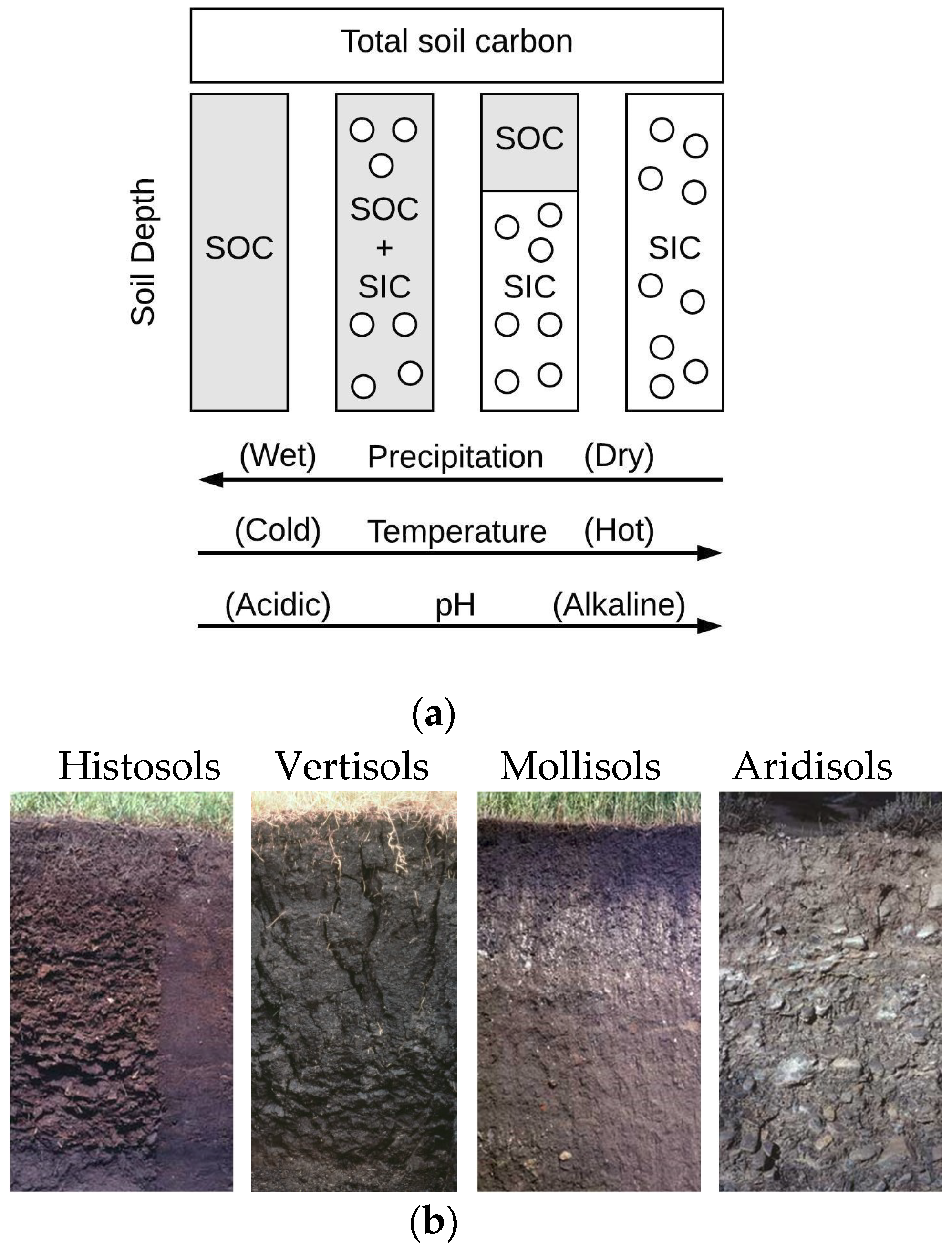
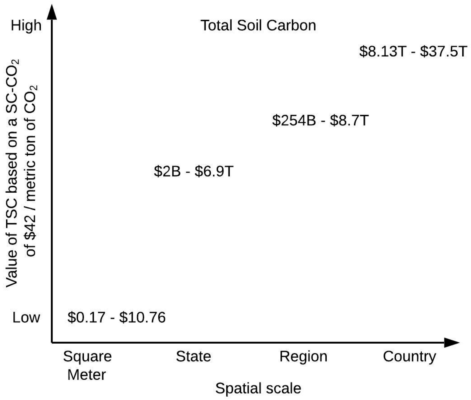
3.1. Value of TSC by Soil Depth in the Contiguous U.S.

The depth with the highest value of TSC storage was the interval 20–100 cm ($9.87T), while the depth with the highest value of TSC area-density was in the same interval 20–100 cm ($1.34 m−2) (Table 5). The interval 0–20 cm had the lowest TSC storage ($4.30T) and lowest area-density ($0.58 m−2) value, which exemplifies TSC’s agricultural utilization in the upper portions of the soil. Share of SOC and SIC in total values of TSC followed the following pattern: 0–20 cm depth (SOC = 85%, SIC = 15%), 20–100 cm depth (SOC = 63%, SIC = 37%), and 100–200 cm depth (SOC = 42%, SIC = 58%).

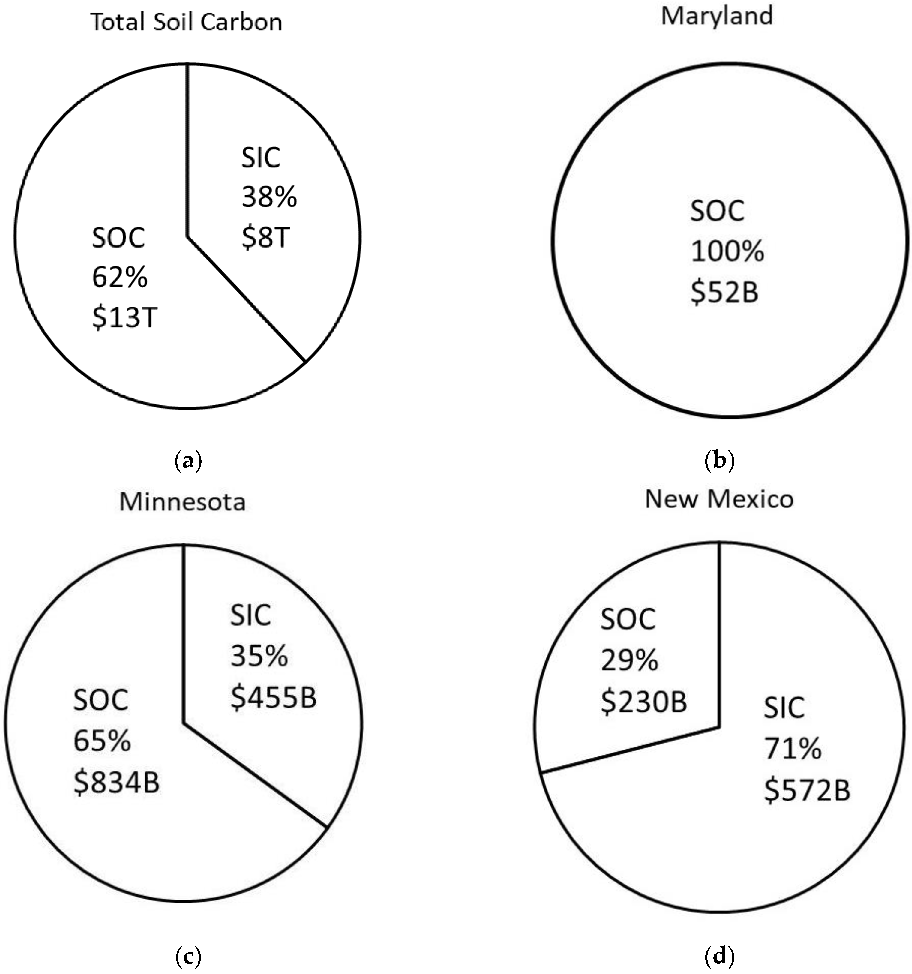
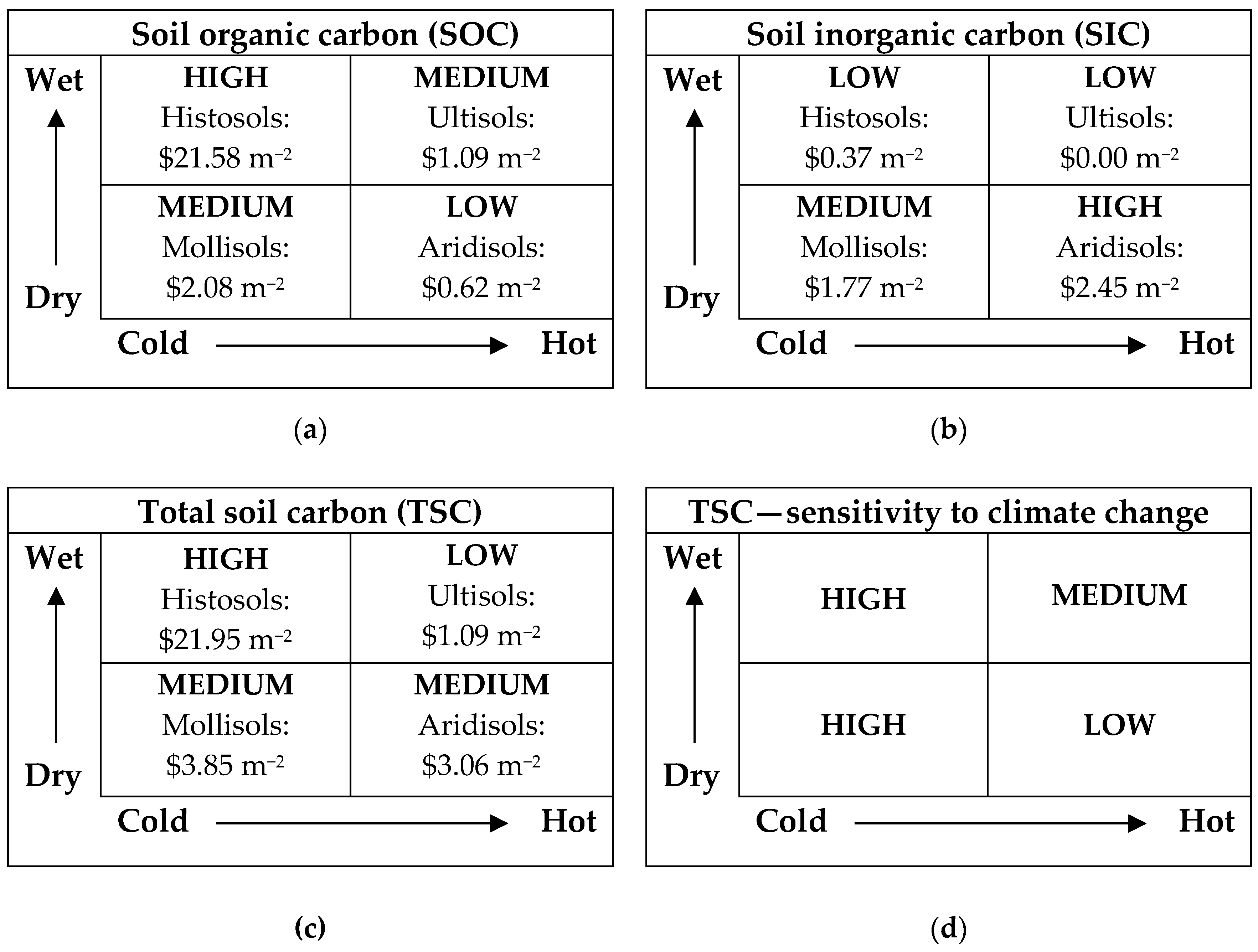
3.2. Value of TSC by Soil Order

The soil orders with the highest TSC storage value were: (1) Mollisols ($7.78T), (2) Aridisols ($2.49T), and (3) Histosols ($2.35T) (Table 6). The value of TSC based on area density within soil order boundaries were ranked: (1) Histosols ($21.95 m−2), (2) Vertisols ($5.84 m−2), and (3) Mollisols ($3.85 m−2) (Table 6). The soil orders with the highest values of TSC storage and area-density were found to be either slightly (e.g., Histosols) or intermediately weathered soils (e.g., Mollisols) (Table 6). Table 7 shows the share of SOC and SIC in total values of TSC with Histosols, Andisols, Spodosol, Ultisols almost solely dominated by SOC, and Aridisols dominated by SIC.

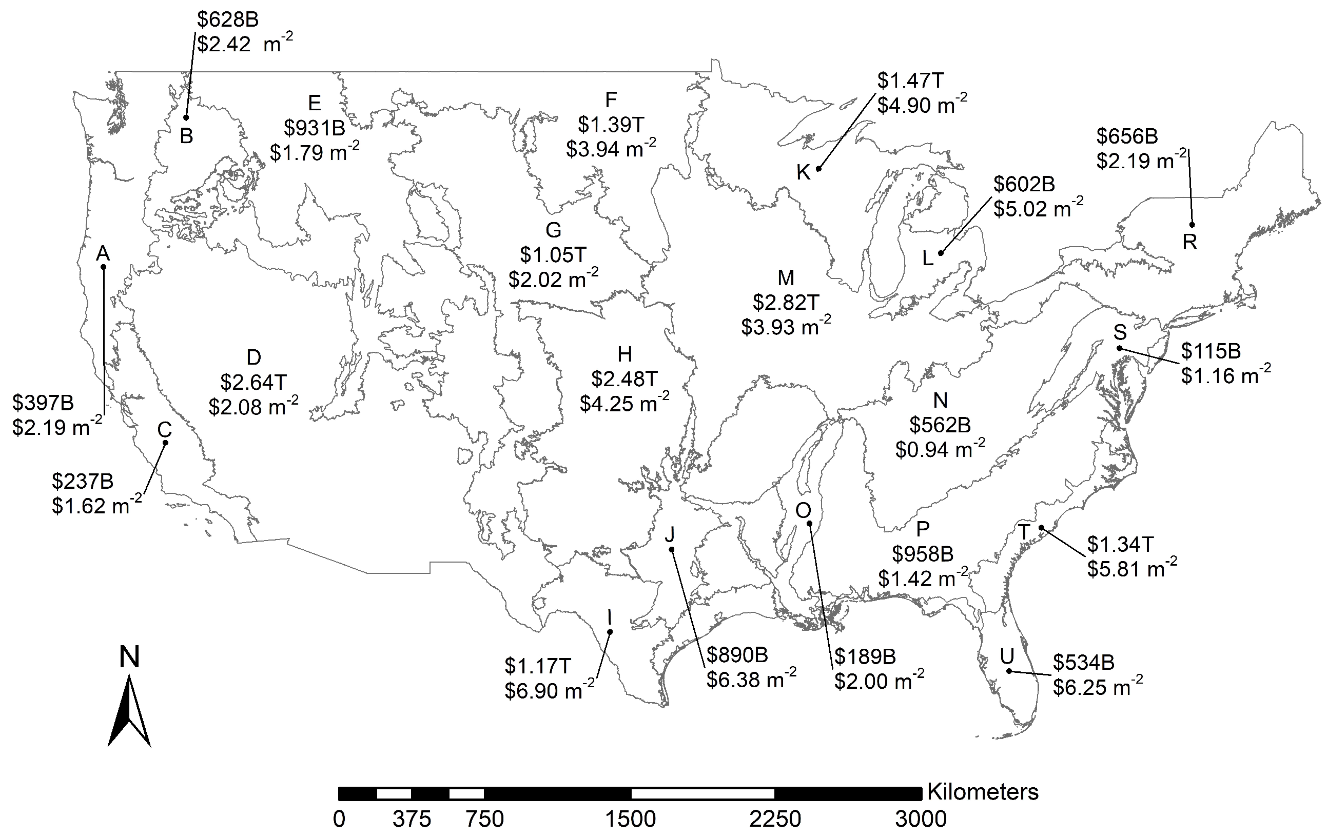
3.3. Value of TSC by Land Resource Regions (LRRs) in the Contiguous U.S.

Land Resource Regions (LRRs) are defined by the U.S. Department of Agriculture (USDA) using major land resource area (MLRA) and agricultural markets, which are denoted using capital letters (e.g., A, B, C, etc.; see Table 8 notes). The contiguous U.S. (with the exception of Alaska and Hawaii) comprises 20 of the 28 LRRs. The LRRs with the highest TSC storage value were: (1) M—Central Feed Grains and Livestock Region ($2.82T), (2) D—Western Range and Irrigated Region ($2.64T), and (3) H—Central Great Plains Winter Wheat and Range Region ($2.48T) (Figure 2). The value of TSC based on area density within LRR boundaries were ranked: (1) I—Southwest Plateaus and Plains Range and Cotton Region ($6.90 m−2), (2) J—Southwestern Prairies Cotton and Forage Region ($6.38 m−2), and (3) U—Florida Subtropical Fruit, Truck Crop and Range Region ($6.25 m−2) (Figure 2).
Share of SOC and SIC in total values of TSC followed the following pattern: A (SOC = 100%), B (SOC = 50%, SIC = 50%), C (SOC = 96%, SIC = 4%), D (SOC = 33%, SIC = 67%), E (SOC = 68%, SIC = 32%), F (SOC = 53%, SIC = 47%), G (SOC = 46%, SIC = 54%), H (SOC = 40%, SIC = 60%), I (SOC = 22%, SIC = 78%), J (SOC = 29%, SIC = 71%), K (SOC = 79%, SIC = 21%), L (SOC = 64%, SIC = 36%), M (SOC = 64%, SIC = 36%), N (SOC = 99%, SIC = 1%), O (SOC = 84%, SIC = 16%), P (SOC = 99%, SIC = 1%), R (SOC = 98%, SIC = 2%), S (SOC = 99%, SIC = 1%), T (SOC = 94%, SIC = 6%), and U (SOC = 98%, SIC = 2%).

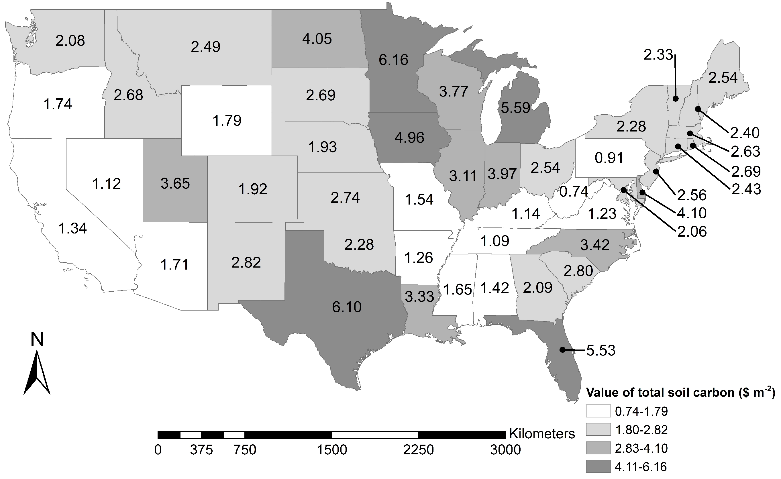
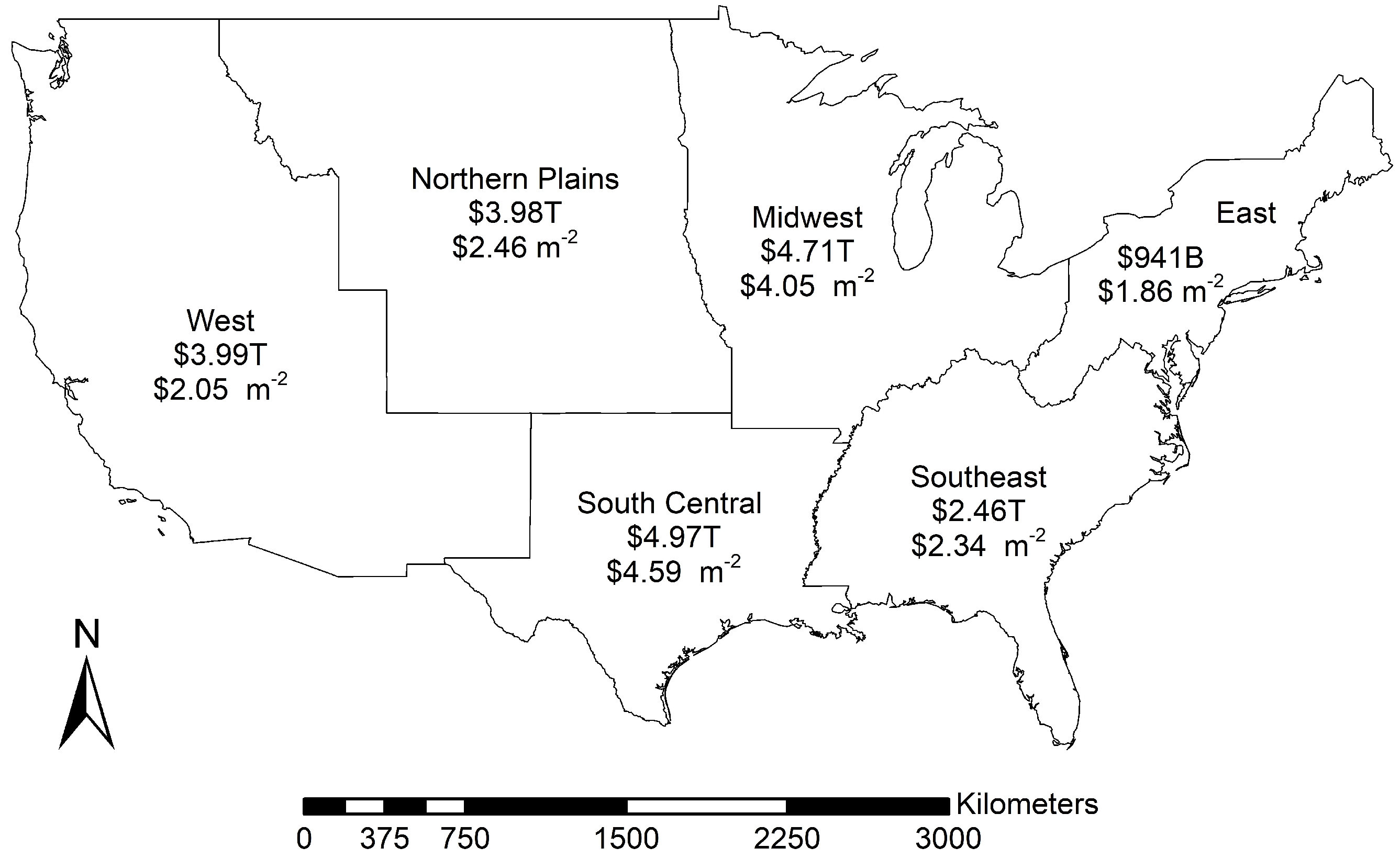
3.4. Value of TSC by States and Regions in the Contiguous U.S.

States with the highest TSC storage value were: (1) Texas ($4.03T), (2) Minnesota ($1.29T), and (3) Montana ($876B) (Figure 3, Table 9). The value of TSC based on area density within state boundaries were ranked: (1) Minnesota ($6.16 m−2), (2) Texas ($6.10 m−2), and (3) Florida ($5.53 m−2) (Table 9, Figure 3). The regions with the highest TSC storage value were: (1) South Central ($4.97T), (2) Midwest ($4.71T), and (3) West ($3.99T) (Table 9, Figure 4). The value of TSC based on area density within regions boundaries were ranked: (1) South Central ($4.59 m−2), (2) Midwest ($4.05 m−2), and (3) Northern Plains ($2.46 m−2) (Table 9, Figure 4). Regionally, share of SOC and SIC in total values of TSC followed the following pattern: East (SOC = 97%, SIC = 3%), Midwest (SOC = 67%, SIC = 33%), South Central (SOC = 37%, SIC = 63%), Southeast (SOC = 99%, SIC = 1%), Northern Plains (SOC = 60%, SIC = 40%), and West (SOC = 50%, SIC = 50%). For states, share of SOC and SIC in total values of TSC followed the following pattern: Delaware, Massachusetts, Maryland, Maine, New Hampshire, New Jersey, Rhode Island, Tennessee, Virginia, North Carolina, Alabama (SOC = 100%, SIC = 0%); Connecticut, West Virginia, Pennsylvania, Georgia, South Carolina (SOC = 99%, SIC = 1%); Florida, Mississippi (SOC = 98%, SIC = 2%); Kentucky (SOC = 97%, SIC = 3%); Vermont, Arkansas (SOC = 96%, SIC = 4%); Louisiana (SOC = 93%, SIC = 7%); New York (SOC = 91%, SIC = 9%); Missouri, Oregon (SOC = 88%, SIC = 12%); California (SOC = 87%, SIC = 13%); Wisconsin (SOC = 84%, SIC = 16%); Nebraska (SOC = 80%, SIC = 20%); Washington (SOC = 78%, SIC = 22%); Kansas (SOC = 74%, SIC = 26%); South Dakota (SOC = 68%, SIC = 32%); Michigan (SOC = 66%, SIC = 34%); Minnesota (SOC = 65%, SIC = 35%); Iowa, Oklahoma (SOC = 64%, SIC = 36%); Illinois (SOC = 63%, SIC = 37%); Ohio (SOC = 62%, SIC = 38%); North Dakota (SOC = 61%, SIC = 39%); Colorado (SOC = 55%, SIC = 45%); Indiana (SOC = 54%, SIC = 46%); Idaho (SOC = 53%, SIC = 47%); Wyoming (SOC = 50%, SIC = 50%); Nevada (SOC = 45%, SIC = 55%); Montana (SOC = 40%, SIC = 60%); Arizona (SOC = 34%, SIC = 66%); New Mexico (SOC = 29%, SIC = 71%); Texas (SOC = 27%, SIC = 73%), and Utah (SOC = 24%, SIC = 76%).

4. Discussion

Economically sustainable soil carbon management requires knowledge of TSC (SOC + SIC), which is important for both provisioning and regulating services (Figure 5). It is important to note that this study is based on the reported values based on recent inventories [9] which represent the SOC and SIC status after the original loss/gain as a result of agricultural and other uses [11]. At the country scale (contiguous U.S.), SOC has a larger share (62%) of TSC value compared to SIC (38%) based on the avoided social cost of carbon, SC–CO2 of $42, U.S. dollars [8]. At the state level, TSC distribution is highly variable due to the influence of the six soil-forming factors (parent material, climate, biota, topography, time, and land use). For example, in Maryland and Delaware, the TSC is mostly SOC according to the STATSGO data (Figure 5).
In Minnesota, SOC has 65% of the total share of TSC compared to 35% of SIC (Figure 5). In New Mexico, SOC has 29% of the total share of TSC compared to 71% of SIC (Figure 5). This variation can be partially explained by the inherent properties of soil types (e.g., soil orders) predominant in the country and states (Figure 6). For example, TSC values for the SC–CO2 vary by soil type with Histosols (common in wetlands) having the highest value ($21.95 m−2) and Ultisols (highly-weathered soils) ($1.09 m−2) having the lowest value, which can be explained by the climate and geographic variation.
This inherent variation also determines the TSC sensitivity to climate change with subsequent gains and/or losses of soil carbon into the atmosphere, which requires soil-specific and carbon-specific (e.g., SOC, SIC) management strategies for increased soil carbon sequestration (Figure 6). For example, plant residues can be added to increase soil carbon sequestration (Table 10), but physical changes during plant residue decomposition will be accompanied by CO2 loss and corresponding social costs ranging from $8/Mg C (after weeks of decomposition) to $29/Mg C (after several years of decomposition) [12]. Soil inorganic carbon sequestration can be achieved by additions of Ca2+ and Mg2+ from outside sources (e.g., atmosphere etc.) (Table 10) and other non-carbonate sources [13]. Similarly to SOC sequestration, SIC sequestration can also be accompanied by CO2 release, especially from the topsoil [13]. Zhao et al. (2018) [14] reported an increase in both SOC and SIC sequestration as a result of additions of wheat straw, wood ash, and/or lime to calcareous soil. According to Mikhailova et al. (2019) [12], long-term soil carbon sequestration may be achieved by getting carbon deeper into the soil where microbial degradation is less compared to the topsoil.
Communicating the value of regulating services provided by soils and TSC in economic terms is crucial for decision-making [15]. Total soil carbon costs can be divided into on-site costs (direct or internal to the user), consisting of TSC losses (e.g., SOC, SIC losses) incurred on the unit of land (e.g., as a result of cultivation), and off-site costs (indirect or external effects on society), consisting of CO2 losses into the atmosphere and affecting society in general [16]. Each additional CO2 loss from the soil can have “cumulative penalties”, generating marginal economic costs for society [16] (Figure 7). These social marginal costs can have an adverse effect of social well-being in the form of social cost of carbon, SC–CO2, therefore it is important to estimate the monetary value of TSC based on SC–CO2. This research estimated the monetary value of TSC based on SC–CO2, which has unidentified market value (little or no market information) (Table 2).
According to Groshans et al. (2019) [4], the unidentified market value of TSC based on SC–CO2 can “either have positive effect (a socially optimal amount should be greater that the current amount) or a negative effect (the socially optimal amount should be less than the current amount) on the costs of climate control after a price for TSC is identified (Table 2)”. Marginal cost curve can be used to represent the cost of climate control for the states based on TSC content. According to Groshans et al. (2019) [4], “the marginal cost curve represents the reduced cost of climate control for the states that contain above a negligible amount of TSC value because the additional benefit of TSC positively impacts carbon sequestration and climate regulation, which decreases the price of climate control, while increasing the quantity.” The beneficial aspects of assessing the value of TSC based on avoided SC–CO2 emissions at various scales (e.g., state, region, LRR, etc.) include identification of the contribution of different types of soil carbon (SOC, SIC) to the CO2 emissions, and assigning the suitable amount of responsibility depending on the TSC values and its individual shares (SOC, SIC), which can potentially lead to more efficient and sustainable use of soil resources. By understanding spatial distributions of TSC, decision-makers can work to maximize the long-term social welfare using an avoided SC–CO2 emissions framework [17]. Monetization of TSC based on avoided SC–CO2 emissions provides decision-makers, and the public, a quantitative context within which assessments can be made about the magnitude and extent of potential soil contribution to C emissions [17]. A monetary context is necessary because it is difficult to understand the actual and potential consequences of how different soil management strategies affect carbon emissions from soil and subsequently could have a long term social cost or benefit. Total soil carbon is necessary for provisioning ecosystem services (e.g., food, fiber production), which provide monetary benefits in the form of agriculutrual and other commodities with market values. However, these provisioning ecosystem services are often associated with CO2 emissions from soil which represent social costs. Costs associated with CO2 emissions are not adequately represented in the marketpace because the costs are born by society and not the producer. Potential changes in world-wide climate may release large quantities of soil C to the atmosphere as CO2, without providing any economic benefit to people [18]. Unlike provisioning services which are tied directly to a production field or area, the social cost does not follow state, regional, or country boundaries. Incorporation of TSC monetary values based on avoided SC–CO2 emissions into the soil survey data enables land managers and policymakers to make informed decisions “that balance goals for production, economics, sustainability, and the environment” [7].
Current soil survey data for TSC have numerous limitations. According to Indorante et al. (1996) [19], soil surveys were designed for production agriculture and natural resource management, and are static in nature, without considering TSC change as a result of various uses and/or environmental changes [7]. Total soil carbon is accumulated over pedogenic time scales (up to a few million years), but can be significantly changed within the human time scales (e.g., over centuries, decades, or less) [7]. Static measurements of TSC found in soil surveys rely on separate measurements of SOC and SIC that are done for representative pedon(s) which are often used to describe large geographic regions [20]. Furthermore, both SOC and SIC vertical distribution data are often extrapolated beyond measured depths. These carbon data are often reported as low, mid-point, and high ranges which result in a wide range of montery SC–CO2 values reported by this study: $8.13T–$37.5T.
Translating TSC stocks into monetary quantities based on the avoided SC–CO2 values allows communication of the social value of TSC to a wide audience (e.g., farmers, banks). Valuation of TSC stocks based on the avoided SC–CO2 values can be useful for future research on factors influencing TSC stocks from a socio-ecological perspective, and efficient allocation of financial resources to areas with the most vulnerable TSC stocks. Limitations in soil survey data require further collection of dynamic TSC measurements preferably within long-term monitoring sites representing a wide range of soils in the areas most sensitive to climate change [21].

5. Conclusions

Carbon sequestered in soils as a total stock of TSC (SOC + SIC) provides regulating ecosystem services (e.g., carbon sequestration and climate regulation), but TSC has not been included in economic valuations of ecosystem services. In this study the regulating services provided by the TSC were valued based on the SC–CO2 in the contiguous United States (U.S.) (with a midpoint valuation of $21.1T) by soil order, depth, state, region, and land resource region (LRR). At the country scale, SOC had a larger share (62%) of TSC value compared to SIC (38%) based on the avoided social cost of carbon, SC–CO2 of $42 U.S. dollars. Soil orders with the highest (midpoint) values for TSC storage were: (1) Mollisols ($7.78T), (2) Aridisols ($2.49T), and (3) Histosols ($2.35T). Soil orders normalized by land area with the highest (midpoint) values for TSC storage were: (1) Histosols ($21.95 m−2), (2) Vertisols ($5.84 m−2), and (3) Mollisols ($3.85 m−2). The majority of the TSC value was associated with the 20–100 cm soil depth interval, with a midpoint value of $9.87T and an area-normalized value of $1.34 m−2. The LRRs with the highest (midpoint) values of TSC storage were: (1) M—Central Feed Grains and Livestock Region ($2.82T), (2) D—Western Range and Irrigated Region ($2.64T), and (3) H—Central Great Plains Winter Wheat and Range Region ($2.48T). States with the highest (midpoint) values for TSC storage were: (1) Texas ($4.03T), (2) Minnesota ($1.29T), and (3) Montana ($876B). States, when normalized by land area, were ranked as: (1) Minnesota ($6.16 m−2), (2) Texas ($6.10 m−2), and (3) Florida ($5.53 m−2). The regions with the highest (midpoint) values for TSC storage were: (1) South Central ($4.97T), (2) Midwest ($4.71T), and (3) West ($3.99T). Region ranking when normalized by land area were: (1) South Central ($4.59 m−2), (2) Midwest ($4.05 m−2), and (3) Northern Plains ($2.46 m−2).
The total values and area-normalized values of TSC stocks were spatially variable, and exhibited variability based on types of soil carbon (SOC, SIC) within TSC (e.g., 100% of TSC for the state of Maryland was SOC). This spatial and compositional distribution information can be used for incentivizing more efficient and sustainable carbon management at various scales and tailored to specific types of soil carbon. In addition, it can be integrated into existing and future decision-support tools, which include other ES valuations.

Author Contributions

Conceptualization, E.A.M.; methodology, G.R.G., M.A.S., and G.C.P.; writing—original draft preparation, G.R.G., and E.A.M.; writing—review and editing, G.R.G., E.A.M., C.J.P., M.A.S., and G.C.P.; visualization, C.J.P.

Funding

This research received no external funding.

Acknowledgments

We would like to thank Bosch, and the reviewers for their constructive comments and suggestions.

Conflicts of Interest

The authors declare no conflict of interest.

References

  1. Keestra, S.D.; Bouma, J.; Wallinga, J.; Tittonell, P.; Smith, P.; Cerda, A.; Montanarella, L.; Quinton, J.N.; Pachepsky, Y.; Van der Putten, W.H.; et al. The significance of soils and soil science towards realization of the United Nations Sustainable Development Goals. Soil 2016, 2, 111–128. [Google Scholar] [CrossRef] [Green Version]
  2. Wood, S.L.; Jones, S.K.; Johnson, J.A.; Brauman, K.A.; Chaplin-Kramer, R.; Fremier, A.; Girvetz, E.; Gordon, L.J.; Kappel, C.V.; Mandle, L.; et al. Distilling the role of ecosystem services in the Sustainable Development Goals. Ecosyt. Serv. 2017, 29, 701–782. [Google Scholar] [CrossRef]
  3. Adhikari, K.; Hartemink, A.E. Linking soils to ecosystem services—A global review. Geoderma 2016, 262, 101–111. [Google Scholar] [CrossRef]
  4. Groshans, G.R.; Mikhailova, E.A.; Post, C.J.; Schlautman, M.A.; Zhang, L. Determining the value of soil inorganic carbon stocks in the contiguous United States based on the avoided social cost of carbon emissions. Resources 2019, 8, 119. [Google Scholar] [CrossRef]
  5. Plaza, C.; Zaccone, C.; Sawicka, K.; Mendez, A.M.; Tarquis, A.; Gascó, G.; Heuvelink, G.B.M.; Schuur, E.A.G.; Maestre, F.T. Soil resources and element stocks in drylands to face global issues. Sci. Rep. 2018, 8, 13788. [Google Scholar] [CrossRef] [PubMed]
  6. Lal, R. Conceptual basis of managing soil carbon: Inspired by nature and driven by science. J. Soil Water Conserv. 2019, 74, 29A–34A. [Google Scholar] [CrossRef] [Green Version]
  7. Tugel, A.J.; Herrick, J.E.; Brown, J.R.; Mausbach, M.J.; Puckett, W.; Hipple, K. Soil change, soil survey, and natural resources decision making: A blueprint for action. Soil Sci. Soc. Am. J. 2005, 69, 738–747. [Google Scholar] [CrossRef]
  8. EPA. The Social Cost of Carbon. EPA Fact Sheet. 2016. Available online: https://19january2017snapshot.epa.gov/climatechange/social-cost-carbon_.html (accessed on 15 March 2019).
  9. Guo, Y.; Amundson, R.; Gong, P.; Yu, Q. Quantity and spatial variability of soil carbon in the conterminous United States. Soil Sci. Soc. Am. J. 2006, 70, 590–600. [Google Scholar] [CrossRef]
  10. Groshans, G.R.; Mikhailova, E.A.; Post, C.J.; Schlautman, M.A.; Zurqani, H.A.; Zhang, L. Assessing the value of soil inorganic carbon for ecosystem services in the contiguous United States based on liming replacement costs. Land 2018, 7, 149. [Google Scholar] [CrossRef]
  11. McNeill, J.R.; Winiwarter, V. Breaking the sod: Humankind, history, and soil. Science 2004, 304, 1627–1629. [Google Scholar] [CrossRef]
  12. Mikhailova, E.A.; Groshans, G.R.; Post, C.J.; Schlautman, M.A.; Post, G.C. Valuation of soil organic carbon stocks in the contiguous United States based on the avoided social cost of carbon emissions. Resources 2019, 8, 153. (In review) [Google Scholar] [CrossRef]
  13. Carmi, I.; Kronfeld, J.; Moinester, M. Sequestration of atmospheric carbon dioxide as inorganic carbon in the unsaturated zone under semi-arid forests. Catena 2019, 173, 93–98. [Google Scholar] [CrossRef]
  14. Zhao, H.; Zhang, H.; Shar, A.G.; Liu, J.; Chen, Y.; Chu, S.; Tian, X. Enhancing organic and inorganic carbon sequestration in calcareous soil by the combination of wheat straw and wood ash and/or lime. PLoS ONE 2018, 13, e0205361. [Google Scholar] [CrossRef] [PubMed]
  15. Robinson, D.A.; Hockley, N.; Dominati, E.; Lebron, I.; Scow, K.M.; Reynolds, B.; Emmett, B.A.; Keith, A.M.; de Jonge, L.W.; Schjønning, P.; et al. Natural capital, ecosystem services, and soil change: Why soil science must embrace an ecosystems approach. Vadose J. 2012, 11, vzj2011.0051. [Google Scholar] [CrossRef]
  16. Telles, T.S.; Dechen, S.C.F.; de Souza, L.G.A.; Guimarães, M.F. Valuation and assessment of soil erosion costs. Sci. Agricola 2013, 70, 209–216. [Google Scholar] [CrossRef]
  17. Paul, I.; Howard, P.; Schwartz, J.A. The Social Cost of Greenhouse Gases and State Policy: A Frequently Asked Questions Guide. Institute for Policy Integrity, New York University School of Law, October 2017. Available online: https://policyintegrity.org/files/publications/SCC_State_Guidance.pdf (accessed on 8 September 2019).
  18. Crowther, T.W.; Todd-Brown, K.E.O.; Rowe, C.W.; Wieder, W.R.; Carey, J.C.; Machmuller, M.B.; Snoek, B.L.; Fang, S.; Zhou, G.; Allison, S.D.; et al. Quantifying global soil carbon losses in response to warming. Nature 2016, 540, 104–108. [Google Scholar] [CrossRef] [PubMed]
  19. Indorante, S.J.; McLeese, R.L.; Hammer, R.D.; Thompson, B.W.; Alexander, D.L. Positioning soil survey for the 21st century. J. Soil Water Conserv. 1996, 51, 21–28. [Google Scholar]
  20. Mikhailova, E.A.; Altememe, A.H.; Bawazir, A.A.; Chandler, R.D.; Cope, M.P.; Post, C.J.; Stigtlitz, R.Y.; Zurqani, H.A.; Schlautman, M.A. Comparing soil carbon estimates in glaciated soils at a farm scale using geospatial analysis of field and SSURGO data. Geoderma 2016, 281, 119–126. [Google Scholar] [CrossRef] [Green Version]
  21. Turetsky, M.R.; Abbott, B.W.; Jones, M.C.; Anthony, K.W.; Olefeldt, D.; Schuur, E.A.G.; Koven, C.; McGuire, A.D.; Grosse, G.; Kuhry, P.; et al. Permafrost collapse is accelerating carbon release. Nature 2019, 569, 32–34. [Google Scholar] [CrossRef] [PubMed] [Green Version]
Figure 1. Types of total soil carbon (TSC) distribution with depth: (a) generalized diagram, with circles representing soil inorganic carbon (SIC), and (b) examples of soil orders (USDA/NRCS) to illustrate TSC distributrion represented in the generalized diagram.
Resources 08 00157 g001
Figure 2. The total (midpoint) values (top number) and midpoint values normalized by area (bottom number) of total soil carbon (TSC) for different Land Resources Regions (LRRs) in the contiguous United States (U.S.), based on TSC numbers from Guo et al. (2006) [9] and a SC–CO2 of $42 per metric ton of CO2 [8].
Resources 08 00157 g002
Figure 3. Midpoint values of total soil carbon (TSC) normalized by land area ($ m−2) for states in the contiguous United States (U.S.), based on TSC numbers from Guo et al. (2006) [9] and a SC–CO2 of $42 per metric ton of CO2 [8].
Resources 08 00157 g003
Figure 4. Total (midpoint) values (top number), and midpoint values of total soil carbon (TSC) normalized by land area (bottom number), for different regions in the contiguous United States (U.S.), based on TSC numbers from Guo et al. (2006) [9] and a SC–CO2 of $42 per metric ton of CO2 [8].
Resources 08 00157 g004
Figure 5. Value of total soil carbon (based on midpoint) by different pools (SOC = soil organic carbon, SIC = soil inorganic carbon): (a) contiguous United States, and selected states ((b) Maryland, (c) Minnesota, (d) New Mexico), based on TSC numbers from Guo et al. (2006) [9] and a SC–CO2 of $42 per metric ton of CO2 [8] (i.e., $ 52 billion U.S. dollars, where B = billion = 109; $13 trillion U.S. dollars, where T = trillion = 1012).
Resources 08 00157 g005
Figure 6. Climate effect on the value of various soil carbon types based on the avoided SC–CO2 of $42 per metric ton of CO2 [8], and SOC sequestration potential: (a) soil organic carbon, SOC (soil orders), (b) soil inorganic carbon, SIC (soil orders), (c) total soil carbon, TSC (soil orders), and (d) TSC sensitivity to climate change.
Resources 08 00157 g006
Figure 7. Scale and cost of total soil carbon (TSC) midpoint values in the contiguous United States (U.S.), based on TSC numbers from Guo et al. (2006) [9] and a SC–CO2 of $42 per metric ton of CO2 [8] (i.e., $ 2 billion U.S. dollars, where B = billion = 109; $6.9 trillion U.S. dollars, where T = trillion = 1012).
Resources 08 00157 g007
Table 1. Types of soil carbon stocks.
Total Soil Carbon Stocks
Separate Constituent StocksComposite (Total) Stocks
SOCSICSOCSICTSC = SOC + SIC
BioticAbioticBioticAbioticBiotic + Abiotic
Note: SOC = soil organic carbon, SIC = soil inorganic carbon, TSC = total soil carbon.
Table 2. Pedosphere–atmosphere ecosystem services exchange, stocks, goods, flows (represented by arrows), and ownership in relation to total soil carbon (TSC) (adapted from Groshans et al. (2019) [4]).
Resources 08 00157 i001
Table 3. Examples of users, scale of use, and probable uses of a SC–CO2 values associated with total soil carbon (TSC) in relation to Sustainable Development Goals (SDGs) (based on Tugel et al. (2005) [7]).
UserScale of UseProbable Uses
Agricultural producersField, farm or ranch, watershed
Minimize negative environmental impacts.
Manage for short-term economic profit and long-term sustainability (cost-benefit analysis).
Land managers (federal, state, local, non-governmental organizations), program managers, policymakersField, watershed, state, regional, national, global
Interpret results of resource assessment and monitoring.
Predict effects of management and climate change on soil functions.
Homeowners, developers, engineers, urban plannersGarden, public works projects, city, county
Prevent land degradation.
Table 4. A conceptual overview of the accounting framework used in this study (adapted from Groshans et al. (2018) [10]).
Biophysical Accounts (Science-Based)Administrative Accounts (Boundary-Based)Monetary Account(s)Benefit(s)Total Value
Soil extentAdministrative extentEcosystem good(s) and service(s)SectorTypes of value
Separate constitute stock 1: Soil organic carbon (SOC)
Separate constitute stock 2: Soil inorganic carbon (SIC)
Composite (total) stock: Total soil carbon (TSC) = SOC + SIC
Soil order
Soil depth
Country
State
Region
Land Resource
Region (LRR)
RegulatingEnvironment: Carbon sequestrationSocial cost of carbon (SC–CO2) and avoided emissions $42 per metric ton of CO2 (2007 U.S. dollars with an average discount rate of 3% [8])
Table 5. Total and area-normalized values of total soil carbon (TSC) by depth for the contiguous United States (U.S.), based on TSC numbers from Guo et al. (2006) [9] and a SC–CO2 of $42 per metric ton of CO2 [8].
Depth (cm)- - - - - - - - - - Total Value - - - - - - - - - -- - - - - - - - - - Value per Area - - - - - - - - - -
Min.
($)
Mid.
($)
Max.
($)
Min.
($ m−2)
Mid.
($ m−2)
Max.
($ m−2)
0–202.06 × 10124.30 × 10127.13 × 10120.280.580.97
20–1003.70 × 10129.87 × 10121.78 × 10130.501.342.41
100–2002.37 × 10126.88 × 10121.26 × 10130.320.931.72
Totals8.13 × 10122.11 × 10133.75 × 1013
Note: Min. = minimum; Mid. = midpoint; Max. = maximum.
Table 6. Total and area-normalized values of total soil carbon (TSC) storage in the upper 2 m within the contiguous United States (U.S.), based on TSC numbers from Guo et al. (2006) [9] and a social cost of carbon (SC–CO2) of $42 per metric ton of CO2 [8].
- - - - - - - - - - Total Value - - - - - - - - - -- - - - - - - - - - Value per Area - - - - - - - - - -
Soil OrderTotal Area
(km2)
Min.
($)
Mid.
($)
Max.
($)
Min.
($ m−2)
Mid.
($ m−2)
Max.
($ m−2)
Slight Weathering
Entisols1,054,0156.04 × 10112.08 × 10123.93 × 10120.571.973.73
Inceptisols787,2546.39 × 10111.70 × 10123.13 × 10120.822.163.97
Histosols107,2491.06 × 10122.35 × 10124.11 × 10129.9321.9538.33
Gelisols-------
Andisols68,6665.05 × 10101.13 × 10111.99 × 10110.741.652.88
Intermediate Weathering
Aridisols809,4231.01× 10122.49 × 10124.36 × 10121.263.065.37
Vertisols132,4333.19 × 10117.72 × 10111.30 × 10122.425.849.83
Alfisols1,274,1027.10 × 10112.32 × 10124.35 × 10120.551.823.42
Mollisols2,020,6943.35 × 10127.78 × 10121.32 × 10131.663.856.55
Strong Weathering
Spodosols250,1331.19 × 10114.96 × 10111.03 × 10120.481.994.10
Ultisols860,1702.52 × 10119.43 × 10111.84 × 10120.291.092.14
Oxisols-------
Totals7,364,1398.12 × 10122.10 × 10133.75 × 1013
Note: Total areas, and thus, the subsequent calculated values, for Oxisols and Gelisols were negligible and, therefore, are not shown. Min. = minimum; Mid. = midpoint; Max. = maximum.
Table 7. Share of soil organic (SOC) and inorganic soil carbon (SIC) in total values of total soil carbon (TSC) storage in the upper 2 m within the contiguous United States (U.S.), based on midpoint SOC, SIC, and TSC numbers from Guo et al. (2006) [9] and a social cost of carbon (SC–CO2) of $42 per metric ton of CO2 [8].
Slight WeatheringIntermediate WeatheringStrong Weathering
Soil OrderSOC (%)SIC (%)Soil OrderSOC (%)SIC (%)Soil OrderSOC (%)SIC (%)
Entisols6238Aridisols2080Spodosols955
Inceptisols6436Vertisols3961Ultisols1000
Histosols982Alfisols6436Oxisols--
Gelisols--Mollisols5446
Andisols991
Table 8. Total and area-normalized values of total soil carbon (TSC) by Land Resource Regions (LRRs) for the contiguous United States (U.S.), based on TSC numbers from Guo et al. (2006) [9] and a SC–CO2 of $42 per metric ton of CO2 [8].
LRRsArea (km2)- - - - - - - - - - Total Value - - - - - - - - - -- - - - - - - - - - Value per Area - - - - - - - - - -
Min.
($)
Mid.
($)
Max.
($)
Min.
($ m−2)
Mid.
($ m−2)
Max.
($ m−2)
A181,2151.63 × 10113.97 × 10117.06 × 10110.892.193.90
B259,2842.79 × 10116.28 × 10111.08 × 10121.082.424.17
C146,8848.49 × 10102.37 × 10114.04 × 10110.571.622.76
D1,268,9221.03 × 10122.64 × 10124.69 × 10120.802.083.70
E521,9943.62 × 10119.31 × 10111.72 × 10120.691.793.30
F351,8425.20 × 10111.39 × 10122.47 × 10121.483.947.04
G521,4424.01 × 10111.05 × 10121.82 × 10120.772.023.50
H583,8201.04 × 10122.48 × 10124.20 × 10121.794.257.19
I169,6894.83 × 10111.17 × 10122.06 × 10122.856.9012.17
J139,6244.24 × 10118.90 × 10111.45 × 10123.036.3810.41
K300,2695.73 × 10111.47 × 10122.68 × 10121.914.908.92
L119,9972.62 × 10116.02 × 10111.04 × 10122.195.028.67
M717,6151.21 × 10122.82 × 10124.73 × 10121.693.936.59
N603,4341.45 × 10115.62 × 10111.16 × 10120.230.941.93
O94,6524.67 × 10101.89 × 10113.76 × 10110.492.003.97
P677,1602.64 × 10119.58 × 10111.80 × 10120.391.422.65
R300,5361.78 × 10116.56 × 10111.38 × 10120.592.194.57
S99,1473.34 × 10101.15 × 10112.38 × 10110.341.162.40
T231,3034.38 × 10111.34 × 10122.54 × 10121.895.8111.00
U85,4101.86 × 10115.34 × 10119.68 × 10112.196.2511.33
Totals7,374,2398.13 × 10122.11 × 10133.75 × 1013
Note: A = Northwestern Forest, Forage and Specialty Crop Region; B = Northwestern Wheat and Range Region; C = California Subtropical Fruit, Truck and Specialty Crop Region; D = Western Range and Irrigated Region; E = Rocky Mountain Range and Forest Region; F = Northern Great Plains Spring Wheat Region; G = Western Great Plains Range and Irrigated Region; H = Central Great Plains Winter Wheat and Range Region; I = Southwest Plateaus and Plains Range and Cotton Region; J = Southwestern Prairies Cotton and Forage Region; K = Northern Lake States Forest and Forage Region; L = Lake States Fruit, Truck and Dairy Region; M = Central Feed Grains and Livestock Region; N = East and Central Farming and Forest Region; O = Mississippi Delta Cotton and Feed Grains Region; P = South Atlantic and Gulf Slope Cash Crops, Forest and Livestock Region; R = Northeastern Forage and Forest Region; S = Northern Atlantic Slope Diversified Farming Region; T = Atlantic and Gulf Cost Lowland Forest and Crop Region; U = Florida Subtropical Fruit, Truck Crop and Range Region; Min. = minimum; Mid. = midpoint; Max. = maximum.
Table 9. Total and area-normalized total soil carbon (TSC) values by state and region for the contiguous United States (U.S.), based on TSC numbers from Guo et al. (2006) [9] and a SC–CO2 of $42 per metric ton of CO2 [8].
State (Region)Area (km2)- - - - - - - - - - Total Value - - - - - - - - - -- - - - - - - - - - Value per Area - - - - - - - - - -
Min.
($)
Mid.
($)
Max.
($)
Min.
($ m−2)
Mid.
($ m−2)
Max.
($ m−2)
Connecticut12,4067.72 × 1093.02 × 10106.55 × 10100.632.435.28
Delaware50434.31 × 1092.06 × 10104.47 × 10100.864.108.86
Massachusetts18,9181.16 × 10105.00 × 10101.07 × 10110.622.635.68
Maryland25,2661.28 × 10105.21 × 10101.11 × 10110.512.064.42
Maine80,5846.50 × 10102.05 × 10114.12 × 10110.802.545.11
New Hampshire22,8011.05 × 10105.50 × 10101.24 × 10110.462.405.45
New Jersey17,7881.62 × 10104.55 × 10109.07 × 10100.912.565.10
New York118,4327.75 × 10102.69 × 10115.52 × 10110.662.284.65
Pennsylvania115,2912.59 × 10101.06 × 10112.29 × 10110.230.911.99
Rhode Island25832.00 × 1096.93 × 1091.48 × 10100.792.705.71
Vermont23,7641.04 × 10105.50 × 10101.24 × 10110.432.335.21
West Virginia61,4481.01 × 10104.60 × 10109.93 × 10100.170.741.62
(East)504,3252.54 × 10119.41 × 10111.98 × 10120.511.863.91
Iowa143,8013.57 × 10117.11 × 10111.11 × 10122.484.967.75
Illinois143,9481.64 × 10114.47 × 10117.88 × 10111.123.115.48
Indiana93,5841.36 × 10113.72 × 10116.67 × 10111.463.977.13
Michigan147,5323.70 × 10118.25 × 10111.41 × 10122.495.599.56
Minnesota209,2235.26 × 10111.29 × 10122.27 × 10122.536.1610.86
Missouri177,4841.06 × 10112.73 × 10114.82 × 10110.591.542.71
Ohio105,4428.49 × 10102.67 × 10115.04 × 10110.802.544.77
Wisconsin140,5422.10 × 10115.30 × 10119.62 × 10111.493.776.84
(Midwest)1,161,5561.95 × 10124.71 × 10128.20 × 10121.694.057.05
Arkansas135,8325.28 × 10101.73 × 10113.28 × 10110.391.262.42
Louisiana109,2737.50 × 10103.63 × 10117.87 × 10110.693.337.21
Oklahoma176,6471.52 × 10114.01 × 10117.03 × 10110.862.283.97
Texas660,6491.73 × 10124.03 × 10126.92 × 10122.626.1010.47
(South Central)1,082,4022.01 × 10124.97 × 10128.74 × 10121.854.598.07
Alabama130,9485.21 × 10101.86 × 10113.57 × 10110.401.422.73
Florida136,4902.67 × 10117.55 × 10111.37 × 10121.975.5310.01
Georgia149,2851.02 × 10113.12 × 10115.70 × 10110.682.093.82
Kentucky101,8473.04 × 10101.17 × 10112.32 × 10110.291.142.29
Mississippi122,5834.30 × 10102.02 × 10113.93 × 10110.351.653.20
North Carolina125,5221.61 × 10114.30 × 10117.77 × 10111.283.426.19
South Carolina78,4896.44 × 10102.19 × 10114.10 × 10110.832.805.22
Tennessee104,2772.59 × 10101.14 × 10112.30 × 10110.251.092.20
Virginia102,7143.33 × 10101.27 × 10112.51 × 10110.321.232.43
(Southeast)1,052,1547.79 × 10112.46 × 10124.59 × 10120.742.344.36
Colorado253,8881.75 × 10114.90 × 10118.78 × 10110.691.933.47
Kansas212,3252.56 × 10115.82 × 10119.53 × 10111.222.744.48
Montana350,8373.85 × 10118.76 × 10111.53 × 10121.092.494.36
North Dakota178,5892.46 × 10117.21 × 10111.32 × 10121.394.057.39
Nebraska198,4191.36 × 10113.82 × 10116.60 × 10110.691.933.33
South Dakota191,9141.89 × 10115.17 × 10119.08 × 10110.992.704.74
Wyoming229,2751.45 × 10114.10 × 10117.35 × 10110.631.793.22
(Northern Plains)1,615,2471.53 × 10123.98 × 10126.98 × 10120.942.464.33
Arizona266,8671.37 × 10114.56 × 10118.55 × 10110.511.713.20
California353,9731.61 × 10114.75 × 10118.61 × 10110.451.342.43
Idaho197,1552.10 × 10115.29 × 10119.62 × 10111.062.684.88
New Mexico284,3583.26 × 10118.01 × 10111.39 × 10121.162.824.88
Nevada269,4151.13 × 10113.05 × 10115.62 × 10110.421.122.08
Oregon239,8761.79 × 10114.16 × 10117.26 × 10110.741.743.03
Utah185,0303.24 × 10116.73 × 10111.10 × 10121.763.655.96
Washington161,8811.48 × 10113.36 × 10115.82 × 10110.922.083.59
(West)1,958,5561.60 × 10123.99 × 10127.04 × 10120.822.053.60
Totals7,374,2388.13× 10122.11 × 10133.75 × 1013
Note: Min. = minimum; Mid. = midpoint; Max. = maximum.
Table 10. Soil carbon classification based on type and carbon sequestration pathway.
Resources 08 00157 i002

