The Markets of Green Cars of Three Countries: Analysis Using Lotka–Volterra and Bertalanffy–Pütter Models

Abstract

Did the diesel scandal of 2015 affect the market for cars? We consider this question in relation to Germany, Austria, and Switzerland. Starting with historical registration data of cars with different drivetrain technologies, we considered each technology in isolation and fitted a five-parameter Bertalanffy–Pütter (BP) growth model to the stocks of cars. We used this model as it generalizes several well-known three-parameter models, which are distinguished by their exponent pair, e.g., Brody model BP (0, 1), West model BP (0.75, 1), and logistic growth BP (1, 2). We then used these models to derive a Lotka–Volterra (LV) model for the co-evolution of the (annual) market shares of the different drivetrain technologies. We augmented this model by a consideration of model uncertainty and found that initially all technologies were in a state of competition, except for Austria, which changed in 2015 to a predator–prey situation with diesel as the sole prey. This analysis of model uncertainty compared the best-fitting growth curve with the growth trajectories of other likely (Akaike weight 5% or higher) models of BP type. We conclude with remarks about open innovation.

1. Introduction

1.1. Background

The use of conventional cars in cities has been criticized for hazardous emissions of nitrogen oxide (NOx) and particulate matter [1]. These emissions are known to trigger asthma, bronchitis, and other respiratory and cardiovascular diseases [2,3]. In response, authorities worldwide have made emission standards more stringent in order to pressure the automotive industry towards developing more environmentally friendly cars.

This legislation raised interest in environmentally friendly alternatives, such as hybrid cars, fuel-cell cars, and battery-driven electric cars [4]. For instance, China has formulated a strategic plan to promote market penetration of battery-powered electric vehicles, aiming at resolving the massive pollution (haze) of its mega-cities as well as reducing dependence on imported oil [5]. In Europe, the green cars initiative developed a roadmap toward electrification, pointing out that the major differences between conventional and green technologies would be the aspects of energy and resource security, climate change, public health, freedom of mobility, and economic growth [6]. The European Commission, too, noted that transport sector electrification would be essential “for meeting the European Union goals of decarbonization and energy security, as it accounts for 25% of all CO₂ emissions in Europe” [7].

1.2. The Diesel Scandal and the Problem of the Paper

In the view of consumers, the turbocharged diesel engine possesses the same power and capacity as the gasoline engine, and it has advantages in terms of torque and fuel economy if used on highways [8]. By promoting diesel cars for these reasons, VW (Volkswagen) became a substantial seller in the USA car market [9]. However, for diesel cars, the strict regulations resulted in the opposite of the expected outcome [10]. During the scandal over VW in 2015, VW was accused of having installed defeat devices in its diesel cars that allowed them to produce more pollution on the road than during laboratory tests. While gasoline cars were made cleaner by three-way catalytic converters [11], VW used nitrogen oxide storage catalytic converters for diesel cars. However, these were of low durability and the defeat device “fixed” this problem [12]. Other car makers soon faced similar charges (BMW, Fiat Chrysler, Ford, General Motors, Mercedes).

In this paper, we ask the following question: Did these events have long-term effects on consumer purchasing behavior? Some authors denied that, in the long run, the diesel scandal would have affected the market standing of diesel cars [13], as “VW recorded strong sales in the years immediately following the scandal” [14]. Furthermore, all means of private transportation may have a negative impact on the environment, including air pollution of traditional fuel driven cars [15], ground-level ozone (O₃) impact from electric cars [16], nuclear disasters from atomic power plants that provide the energy needed for electric cars [17], as well as global warming caused by methane (CH₄), if animal-pulled carriages would replace conventional vehicles. Perhaps consumers might be overtasked if they were asked to consider all these environmental concerns in their decision-making. Indeed, consumers may have purchased diesel cars because they deemed them to be more environmentally friendly than their gasoline counterparts. This was the case when, two decades ago, greenhouse gas emerged as a global policy issue (1997 Kyoto Protocol): diesel vehicles were promoted because they had lower carbon dioxide (CO₂) emissions per kilometer [18,19].

We analyze the long-term dynamics of the car market of three countries in more detail, namely Germany, Austria, and Switzerland. Germany is renowned for its automotive industry, which employs about 0.8 M people (data for 2012: [20]). In Austria and Switzerland, each with around a tenth of the German population, the automotive industries employ around 32,000 and 34,000 people, respectively. We selected these countries because VW is a German-based company. Furthermore, other than in the USA, where VW offered adequate compensation [21], consumers of the three countries had to sue VW for compensation. Only recently did the Federal Supreme Court of Germany (25 May 2020, case VI ZR 252/19) rule that VW must recall its cars.

2. Methods

2.1. Outline of the Approach

The progress in the analytic methods for market diffusion is illustrated by the proliferation of models, but there is no consensus on the best of these approaches [22]. In this paper, we aim at modeling the growth of the stock of cars with different drivetrain technologies (

Table 1. Annual car registrations.

	Year	Hybrid	Electric	Liquid Gas	Natural Gas	Petrol	Diesel
Austria	2011	1310	631	-	262	159,027	194,721
	2012	2171	427	-	274	143,325	189,622
	2013	2573	654	-	455	134,276	180,901
	2014	1823	1281	-	279	126,503	172,381
	2015	2241	1677	-	167	122,832	179,822
	2016	3324	3826	-	119	131,756	188,820
	2017	6483	5433	-	114	163,701	175,458
	2018	7473	6757	-	110	184,150	140,111
	2019	14,304	9242	-	421	176,706	126,311
Germany	2012	21,438	2956	11,465	5215	1,555,241	1,486,119
	2013	24,963	6051	6255	7835	1,502,784	1,403,113
	2014	22,908	8522	6234	8194	1,533,726	1,452,565
	2015	22,529	12,363	4716	5285	1,611,389	1,538,451
	2016	47,996	11,410	2990	3240	1,746,308	1,539,596
	2017	55,239	25,056	4400	3723	1,986,488	1,336,776
	2018	98,816	36,062	4663	10,804	2,142,700	1,111,130
	2019	175,969	63,281	7256	7623	2,136,891	1,152,733
Switzerland	2005	-	13	-	442	185,120	74,114
	2006	1272	9	-	1064	185,807	80,857
	2007	3220	19	-	1653	185,055	92,333
	2008	3092	24	-	1136	189,151	93,366
	2009	3900	57	-	1063	182,174	78,755
	2010	4250	201	-	721	200,576	90,547
	2011	5462	452	-	651	211,540	109,324
	2012	6708	924	-	519	200,576	124,911
	2013	7158	1392	-	791	185,070	115,656
	2014	6893	1948	-	1041	180,875	113,304
	2015	8785	3882	-	1080	185,469	127,899
	2016	10,587	3525	-	944	178,666	125,595
	2017	11,846	4929	-	769	183,637	113,848
	2018	15,432	5411	-	805	188,847	90,360
	2019	26,376	13,197	-	1252	192,430	79,618

Sources: Compiled by the authors using internet resources [25,26,27].

). For this type of problem, trend models, such as logistic growth, are common [5,23]. We improve this by using the Bertalanffy–Pütter (BP) growth model, which generalizes the common trend models and therefore achieves a better fit. In the initial step, we model the growth curves of each drivetrain technology independently of the other technologies by using the BP model to describe its stock (y) of cars over time (t). The growth functions y(t) of the BP model are solutions of the differential Equation (1) of Pütter [24]. The parameters of the model are determined from fitting the growth curve to data (details below and in

Table 2. Parameters for Equation (1) with best fit to the stock of cars (computed from Table 1).

Country		Typeof Car	Best-Fit Parameter of the BP Model					Goodness of Fit			Data Characteristics
			a	b	c	p	q	SSE	R2 (%)	NRMSE (%)	Count n	Grid Size	Mean
Austria	AT	Petrol	0.27	0.60	1.83 × 105	3.90 × 103	3.21 × 10−1	2.22 × 109	99.82	2.19	9	3.94 × 104	7.17 × 105
		Diesel	0.11	3.02	2.01 × 105	4.41 × 104	1.79 × 10−14	4.62 × 108	99.97	0.79	9	3.94 × 104	9.06 × 105
		Electric	1.25	1.37	6.04 × 102	2.27 × 10−1	5.89 × 10−2	2.60 × 105	99.97	1.82	9	3.99 × 104	9.34 × 103
		Nat. Gas	0.00	0.23	2.50 × 102	9.73 × 102	1.45 × 102	7.15 × 104	97.63	6.85	9	3.94 × 104	1.30 × 103
		Hybrid	1.12	1.13	2.85 × 103	1.70 × 10−1	5.47 × 10−2	5.01 × 106	99.63	5.11	9	3.96 × 104	1.46 × 104
Switzerland	CH	Petrol	0.19	0.76	1.87 × 105	1.86 × 104	1.70 × 100	1.09 × 109	99.99	0.56	15	3.94 × 104	1.51 × 106
		Diesel	0.35	3.30	9.15 × 104	1.09 × 103	2.78 × 10−16	1.63 × 109	99.95	1.35	15	4.46 × 104	7.70 × 105
		Electric	0.88	0.89	2.23 × 101	2.10 × 100	8.11 × 10−1	7.04 × 106	99.56	9.45	15	3.92 × 104	7.25 × 103
		Nat. Gas	0.00	0.17	6.63 × 102	1.84 × 103	2.08 × 102	1.36 × 106	99.41	4.05	15	3.94 × 104	7.45 × 103
		Hybrid	0.80	0.81	4.47 × 103	3.12 × 100	1.14 × 100	6.94 × 107	99.55	5.61	14	3.94 × 104	3.97 × 104
Germany	GE	Petrol	0.24	0.27	1.58 × 106	4.15 × 104	1.50 × 10−1	3.91 × 1010	99.97	0.94	8	3.86 × 104	7.45 × 106
		Diesel	0.64	0.95	1.51 × 106	2.57 × 102	1.48 × 100	1.10 × 1010	99.99	0.57	8	3.94 × 104	6.46 × 106
		Electric	1.00	1.01	6.56 × 103	7.08 × 10−1	2.23 × 10−1	3.36 × 107	99.84	3.77	8	3.94 × 104	5.44 × 104
		Nat. Gas	0.10	0.36	6.78 × 103	2.64 × 103	2.75 × 101	3.24 × 107	98.05	7.14	8	3.94 × 104	2.82 × 104
		Liq. Gas	0.00	0.60	1.23 × 104	5.97 × 103	2.28 × 100	9.27 × 106	99.08	3.61	8	3.96 × 104	2.98 × 104
		Hybrid	1.14	1.15	3.29 × 104	7.44 × 10−2	4.57 × 10−4	2.56 × 108	99.84	3.41	8	3.94 × 104	1.66 × 105

):

$$y^{\prime }\left(t\right)=p·y{(t)}^a-q·y{(t)}^b$$

(1)

We then ask if perhaps a simpler model might suffice, using three instead of five parameters; examples are the logistic and the Gompertz growth models.

Trend models have the disadvantage that they investigate single products in isolation. We therefore continue with a system dynamic approach [28] that uses a generalized Lotka–Volterra (LV) system of differential Equation (2) to model the dynamics of the market shares of the competing drivetrain technologies. We use this model to unveil otherwise hidden changes in the characteristics of the market dynamics of the three countries. Thereby, one of the technologies (index i = 0) is the outside, which supposedly does not affect the market dynamics. For the other technologies, the market shares z_i(t) interact as in Equation (2). We will use the BP model to find suitable coefficients g_i(t) for the LV equations (details below).

$$\frac{z_i^{\prime }\left(t\right)}{z_i\left(t\right)}=g_i\left(t\right)-{\displaystyle \sum }_{j\ge 1}{g}_j\left(t\right)·z_j\left(t\right)\begin{array}{cc}\mathrm{for}& i\ge 1\end{array}$$

(2)

Finally, to justify our conclusions about the changes in the character of the market dynamics, we analyze model uncertainty and proceed with simulations of the car market (

Table 3. Percent (and percent of total weight) of simulations resulting in certain scenarios.

Scenario		2013	2014	2015	2017	2019	2021
Pairwise competition	AT	t = 2:1 70% (88%)	t = 3.5: 100% (100%)	t = 4.5: 99% (100%)	t = 6.5: 98% (97%)	t = 8: 97% (92%)	t = 10: 45% (45%)
	CH	t = 8: 98% (99%)	t = 9.5: 76% (78%)	t = 10.5: 12% (7%)	t = 12.5: −	t = 14: −	t = 16: −
	DE	t = 1: 75% (86%)	t = 1.5: 58% (74%)	t = 2.5: 30% (41%)	t = 4.5: 4% (2%)	t = 7: 35% (18%)	t = 9: 18% (15%)
Diesel as the sole prey	AT	t = 2: 6% (2%)	t = 3.5: −	t = 4.5: 1% (0%)	t = 6.5: 2% (3%)	t = 8: 3% (8%)	t = 10: 2% (4%)
	CH	t = 8: −	t = 9.5: 21% (20%)	t = 10.5: 84% (90%)	t = 12.5: 93% (91%)	t = 14: 88% (84%)	t = 16: 46% (50%)
	DE	t = 1: 12% (4%)	t = 1.5: 24% (12%)	t = 2.5: 54% (49%)	t = 4.5: 94% (97%)	t = 7: 62% (80%)	t = 9: 14% (31%)
Diesel and petrol as the sole prey	AT	t = 2: 24% (10%)	t = 3.5: −	t = 4.5: −	t = 6.5: −	t = 8: −	t = 10: −
	CH	t = 8: −	t = 9.5: 3% (2%)	t = 10.5: 4% (3%)	t = 12.5: 7% (9%)	t = 14: 12% (16%)	t = 16: 10% (18%)
	DE	t = 1: 8% (5%)	t = 1.5: 17% (12%)	t = 2.5: 16% (10%)	t = 4.5: 2% (1%)	t = 7: 3% (2%)	t = 9: 1% (0%)

Notes for both tables: accuracy to the last decimal displayed; grid size is the number of grid points (yellow dots in Figure 1) used; ¹: time t of the model (for different data the same year corresponds to different t), followed by the percent of simulations, with the indicated result and (in brackets) of the total weight, or by “−“ if the scenario is rare.

) using certain three-parameter models with a nearly best fit. We thereby define “nearly best fit” using the Akaike [29] information criterion (roughly, it identifies the likely models and, for the model curves, there is barely a visible difference to the data.) We think that the conclusions drawn from model uncertainty are more reliable when compared to conclusions drawn from a parameter variation with randomly varied parameters, since we use only models with the best fit to given data.

2.2. Data

For Table 1, we retrieved the annual registrations (sales figures of new cars) from publicly available online resources. We distinguished gasoline-powered cars, diesel cars, electric cars, hybrid cars, and cars powered by natural gas or liquid gas (liquified petroleum gas). To make the data comparable, we combined certain data (e.g., hybrid cars using gasoline or using diesel) and we ignored rare technologies (e.g., Switzerland counted vehicles without a motor). Note that, for Switzerland, the data for hybrid cars were not available for the first year.

As growth models in general are not suitable in situations where growth and decay both occur, we modeled the stock of cars. We therefore used Table 1 to compute the accumulated registration data for the mentioned technologies. If x₁, x₂, x₃, …are the registrations from successive years t₁, t₂, t₃, … (Table 1), then the stock is y₁ = x₁, y₂ = y₁ + x₂, …, y_k = y_k−1 + x_k (sum of new sales from the first year until present). We thereby also achieve a smoothening of the data. For the modeling, we represent the years by t₁ = 0, t₂ = 1, t₃ = 2, … (except for hybrid CH: t₁ = 1, as the other CH time series started one year earlier).

2.3. BP Model

We use the BP growth model, differential Equation (1), to describe the stock y(t) of cars over time. Equation (1) can be solved analytically, though, in general, not by means of elementary functions [30]. The parameters of the model (Table 1) are the exponent pair a < b, non-negative constants p and q, and the initial value y(0) = c > 0, where, for each country, t = 0 is the first year of its data (t = 1 for Swiss hybrid cars). They are determined from fitting the growth curve to data; see Table 2. As we optimize also for the initial values c, the best-fit values for c in Table 2 will slightly differ from the observed initial registration data in Table 1.

2.4. Other Growth Models

In the literature, there are several other five-parameter growth models, such as the model of Bass [31] for market diffusion, which has also been used to model the diffusion of electric cars [32]. We decided to use the BP model as it is known to be flexible [33] and as it includes as special cases several simple three-parameter models which have been used previously in the analysis and forecasting of technology diffusion and business trends [34,35]. Specifically, the modeling of the automotive market has often used logistic growth [5,23] or the Gompertz model [36,37,38].

Certain named three-parameter models are defined from (1) by specifying certain exponent pairs (Figure 1: blue dots). Each pair (a, b) defines a unique BP model BP(a, b) with three free parameters, such as the logistic growth model BP(1, 2) of Verhulst [39], the Brody [40] monomolecular model BP(0, 1) of bounded exponential growth, the von Bertalanffy [41,42] model BP(1, 2/3), or the more recent West [43] model BP(1, 3/4). The Richards [44] model and the generalized Bertalanffy model are classes of BP models (a = 1, b > 1 and b = 1, a < 1, respectively).

The Gompertz [45] model is the limit case BP(1, 1) with a different differential equation, where b converges to a = 1 from above [46]. When we compare the Gompertz model with other BP models, we use BP(1, 1.01) as a proxy for the Gompertz model.

2.5. Sales and Market Shares

Starting with the BP model curve y_i(t) fitted to the stock of cars using a certain drivetrain technology (i), we use the derivative y_i′ as the model curve for the current annual sales x_k+1 (at time t_k+1 = k, k = 1, 2, …), because x_k+1 = y_k+1 – y_k ≈ y_i(t_k+1) − y_i(t_k) = y_i(k) – y_i(k − 1) = y_i′(k − ζ) for some ζ (intermediate value theorem). For simplicity, we replace ζ by a fixed time shift 0 ≤ ts_i ≤ 1 for all k ≥ 1; i.e., we model sales x_k+1 by the function y_i′ (k − ts_i).

To obtain the time shift ts_i, we use the method of least squares, minimizing the sum of squared errors between x_k+1 and y_i′ (k − ts_i), where y_i is the best-fit BP growth function; see

Table 4. Time shifts to relate market shares and the derivatives of the BP growth functions.

Ctry.	ts0	ts1	ts2	ts3	ts4
	Gas	Hybrid	Electric	Petrol	Diesel
AT	0.39	0.42	0.50	0	0.33
CH	1	0.09	0.34	1	0.22
DE	0	0.44	0.45	0.40	0.50

. The market share s_i(t) at time t is then given by Equation (3), where the total current sales are the market volume m(t):

$$\begin{array}{cc}\begin{array}{cc}{s}_i\left(t\right)=\frac{y_i^{\prime }\left(t-t{s}_i\right)}{m\left(t\right)}& \mathrm{and}\end{array}& m\left(t\right)={\displaystyle {\displaystyle \sum }_{i\in \mathrm{technologies}}}{y}_i^{\prime }\left(t-t{s}_i\right)\end{array}$$

(3)

The computations related to the market shares for Germany use the combined data for natural and liquid gas cars. This ensures that the market dynamics of different countries are compared using the same number of comparable technologies

2.6. LV Model

Lotka [47] and Volterra [48] introduced a system of differential equations to model the dynamics of competing species. Despite its simplicity, this model displays a multitude of possible patterns of co-existence [49] that made it an attractive model of economic competition [50,51]. Here, we use the Lotka–Volterra (LV) system (2) with variable coefficients, as, for this system, there is an explicit solution [52,53]. Variable coefficients are used as they represent situations where companies may actively influence the competitive roles of their products (e.g., PR and marketing, technological advances).

One of the technologies (index i = 0) is selected as the outside. Generally, this is the technology with the lowest market share. For the other technologies, we use the market shares s_i(t) from above to define certain functions f_i and g_i; see Equation (4). For i ≥ 1, the market shares are then solutions s_i(t) = z_i(t) of the LV system (2) with these coefficients g_i. The market share z₀(t) is the difference to 100% of the sum of the z_i(t), i ≥ 1 (remainder of the market); z₀ = s₀.

$$\begin{array}{cc}{f}_i\left(t\right)=\ln \left(s_i\left(t\right)\right)-\ln \left(s_0\left(t\right)\right)& \begin{array}{ccc}\mathrm{and}& g_i\left(t\right)=f_i^{\prime }\left(t\right)& \begin{array}{cc}\mathrm{for}& i\ge 1\end{array}\end{array}\end{array}$$

(4)

This model has an economic meaning [54]: f_i are the (assumed) utilities of consumers for different drive technologies (the utility of the outside good i = 0 is 0) and, if consumers maximize their utility, then Equation (2) describes the market shares. Amongst economic applications are, e.g., studies of the competition between tourism destinations [55] or between ports [56,57].

We use this model to identify the competitive market characteristics [52]. If the two coefficients g_i(t) and g_j(t) are positive, then, at time t, the two technologies (i, j) are in a state of competition. If all coefficients g_i(t) of Equation (2) are positive, this is a state of pairwise competition. This means that (at time t) more sales of cars using any other technology reduce the growth of the own market share. In the absence of other technologies, the own market share would grow. If one of the two coefficients g_i(t) or g_j(t) is positive and the other is negative, then the two technologies are in a predator-prey situation. The technology with the negative coefficient is the prey, the other one the predator, whereby more prey enhances the growth of the predator and more predators inhibit the growth of prey. (Other than in the classical ecological predator–prey model, in this model, the market shares of predators/prey would grow/decrease also in the absence of prey/predators, whence the process is not circular.) If both coefficients g_i(t) and g_j(t) are negative, then the two technologies are in a situation of mutualism (symbiosis), where the presence of the other technology enhances the own growth. The exceptional cases, where one or both coefficients vanish, are characterized as commensalism, amensalism, and neutralism. These cases were observed for LV models of innovation diffusion [58].

2.7. Calibration

We use various measures for the goodness of fit. They are all related to the sum SSE of squared errors: when fitting the BP growth function to the stock of cars, we seek parameters that minimize SSE. Thereby, if y(t) is a solution of Equation (1), using certain exponents a < b and parameters p, q, c, if y_k are the stock data at time t_k, and if n is the number of data, then SSE is defined by Equation (5).

$$\begin{array}{c}SSE={\displaystyle {\displaystyle \sum }_{k=1}^n}{\left(y_k-y\left(t_k\right)\right)}^2\end{array}$$

(5)

In Equation (6), RMSE is the root-mean-squared-error and NRMSE is the normalized RMSE (as percent of the mean). R-squared (R²) of Equation (7) is the coefficient of determination that compares the model fit with the fit by the trivial constant model.

$$\begin{array}{cc}\begin{array}{cc}RMSE=\sqrt{SSE/n}& \mathrm{and}\end{array}& NRMSE=\frac{RMSE}{\mathrm{mean}\left(y_1,y_2,\dots y_n\right)}\end{array}$$

(6)

$$\begin{array}{c}{R}^2=1-\frac{SSE}{{{\displaystyle \sum }}_{k=1}^n{\left(y_k-\mathrm{mean}\left(y_1,y_2,\dots y_n\right)\right)}^2}\end{array}$$

(7)

2.8. Data Fitting

Standard optimization tools (e.g., NonlinearModelFit of Mathematica) may not always find best-fit parameters for model (1). The literature has reported problems already for the simpler Richards model [59]. This paper uses a grid-search strategy for data fitting. It identifies the best-fit parameters for 4 × 10⁴ three-parameter models BP (a, b) using exponent pairs (a, b) on a certain grid, the yellow area in Figure 1. Figure 2 plots these growth curves (they cover the yellow area) together with the best-fit curve corresponding to the best-fit exponent pair (black).

The search starts with a grid (step size 0.01 in both directions) of exponent pairs (Figure 1). For each grid point (a, b), we seek the best-fit parameters (p, q, c) for the three-parameter model BP (a, b); the so minimized sum of squared errors is SSE_opt (a, b). This optimization uses a custom-made variant of the method of simulated annealing [60,61]. The outcome of optimization is exported into a spreadsheet (its columns list a, b, c, p, q, and SSE). The best-fit parameters (a_min, b_min, c_min, p_min, q_min) of the grid are identified from the row with the lowest value of SSE. This defines the overall lowest SSE of (1) as SSE_min = SSE_opt (a_min, b_min). If the best-fit exponent pair is on the upper or left boundary of the grid, then we enlarge the grid near this boundary and repeat the search, until an optimal inner point is found. This optimizes the exponents a_min, b_min with an accuracy value of 0.01 (for the other parameters, we use a higher accuracy value.)

2.9. Model Uncertainty

For each type of technology and each country, there is a different best-fit model for the growth of the stock of cars. We now ask if a simpler modeling approach is feasible: is there one exponent pair (a, b), so that BP (a, b) has a good fit to all growth data? For instance, can all growth curves be modeled by the often-used logistic model? We use two approaches to address this question. One measures goodness of fit in terms of R², the coefficient of determination. It asks which R² values were obtained for the data using a specific model.

The second approach focuses on the models that are likely to be true. In Equation (8), AIC is the Akaike [29] information criterion; it penalizes models that use more parameters (overfitting), whereby the number p of parameters also counts SSE (e.g., p = 4 for the logistic model). Given a finite set of models, the Akaike weight prob compares a given model with the overall best-fit model (it has the lowest AIC: AIC_min). Assuming that either the best-fit model or the given model is true, then prob is the probability (maximum: 50%) that the given model is true despite its poorer fit [62]. As in Figure 1 (red area), we then identify all models with an Akaike weight of 5% or higher.

$$\begin{array}{ccc}AIC=n·\ln \left(\frac{SSE}{n}\right)+2·p& \mathrm{and}& \mathrm{prob}=\frac{\exp \left(-\frac{AIC-AI{C}_{min}}{2}\right)}{1+\exp \left(-\frac{AIC-AI{C}_{min}}{2}\right)}\end{array}$$

(8)

2.10. Simulation

Finally, we explore the extent to which the growth trajectories depend on the choice of growth model (model uncertainty). To this end, we use a Monte Carlo simulation to identify the growth patterns of the likely growth curves (red area in Figure 2). To avoid a “junk in–junk out” situation from a simulation with generally false models, we exclude models from the simulation that are unlikely to be true. Thus, we select at random 5000 exponent pairs (a, b) of the grid (red area in Figure 1) so that the model BP(a, b) has an Akaike weight (probability to be true) of prob > 5% when compared to the best-fit model BP(a_min, b_min). We therefore do not penalize the best-fit model for the optimization of the two exponents, as the optimization was merely a comparison of a given finite set of three-parameter models defined by a search grid. (Thus, in formula (8), we use p = 4 to count the parameters c, p, q, and SSE; n is the number of time-points.) The upper and the lower function values of the 5000 best-fit growth curves then define the band of the growth scenarios that can be obtained from the likely models (Figure 2 and Figure 3, red area).

We apply the simulation approach to identify the most likely scenarios for the competition between the different technologies. To this end, for each technology, we select at random a growth curve with Akaike weight of at least 5% and we combine these growth curves to define the market shares and the corresponding LV equations. We then classify for each simulated dynamic model its pattern of competition (scenario) at a given moment in time. The outcome indicates the percentage of the 5000 simulations for which a certain scenario is observed. We are particularly interested in three scenarios: pair-wise competition of all technologies (meaning business as usual), diesel as the sole prey (perhaps a consequence of the diesel scandal), and diesel together with petrol as the sole prey (a preference of consumers for green technologies). In addition, we inform about the relative weights of the scenarios. Therefore, the weight of a simulation is the product of the Akaike weights of the selected growth functions for the different technologies. The total weight is the sum of the weights of all 5000 simulations.

3. Results

3.1. Graphical Review of Methodology

Figure 1, Figure 2, Figure 3, Figure 4 and Figure 5 explain our methodological approach for a concrete example, the electric car data from Austria (Table 1). The grid search has reduced optimization to the search for the best-fitting model amongst those with exponent pairs in the search grid (yellow area in Figure 1). The blue dots in Figure 1 are the exponent pairs of certain named three-parameter growth models. The black dot is the exponent pair (a_min, b_min) of the best-fit model. None of the exponent pairs of the named models have been close to this optimal exponent pair. The red area of Figure 1 collects 22,442 exponent pairs of BP models with an Akaike weight of 5% or higher when compared to the best-fit model. The frayed appearance of the red area reflects the random character of simulated annealing; it leads to slight fluctuations of the accuracy for different grid points.

Figure 2 plots the stock (accumulated registration data) of electric cars (AT) during the years 2011–2019 (blue) and the best-fit BP growth curve to these data (black). It corresponds to the black exponent pair and uses the best-fit exponents from Table 2. The yellow and red bands in Figure 2 summarize the outcomes of Monte Carlo simulations: it displays, for discrete points in time (t = 0, 1, …, 10), the minimum and maximum of the function values of the 5000 randomly selected growth functions whose exponent pairs come from the yellow and red areas of Figure 1, respectively. The figure connects these points by lines and the intermediate area is shaded accordingly. The yellow area is relatively broad, as it includes also poorly fitting models. However, as each of the randomly selected model curves is a best-fit curve subject to the choice of the exponent pair, the yellow area is not too remote from the data-points. The red band (growth curves of other likely models) is close to the data.

Figure 3 compares the data of Table 1 for electric cars (AT) with the derivatives of the best-fit curve and the curves from the random sample with red exponent points (Figure 1). Table 4 lists the used time shifts. For the simulations, we used the same time shift ts as for the best-fit model. For the annual sales data (x₂, x₃, …, x₁₀ of Table 1), the fluctuations around the model curve y′(t–ts) are much higher than the fluctuations of the accumulated data y_n around the BP growth curve y(t). However, as the red band (sales data from other likely models) is wide, high fluctuations are to be expected.

Figure 4 compares the market shares for electric cars (AT) with Formula (2), the estimate for the market shares using the best-fit model. As the market share cannot be computed in isolation, this computation uses the best-fitting growth curves for all technologies. The computation of the red band of the most likely market shares uses 5000 simulations, where, for each technology, one best-fitting BP-growth curve is selected at random. More specifically, for each technology, one exponent pair (a, b) in the red region (of the analogue to Figure 1) is selected at random and the growth curve from the model BP(a, b) with the best fit to the data of the technology is used.

Figure 5 plots the consumers’ utility for electric cars (AT) based on the best-fit models for the market shares with gas cars as the outside goods. It compares this curve to the range of the other likely utilities. A common observation for all best-fit utility functions for all countries was their approximately parabolic shape.

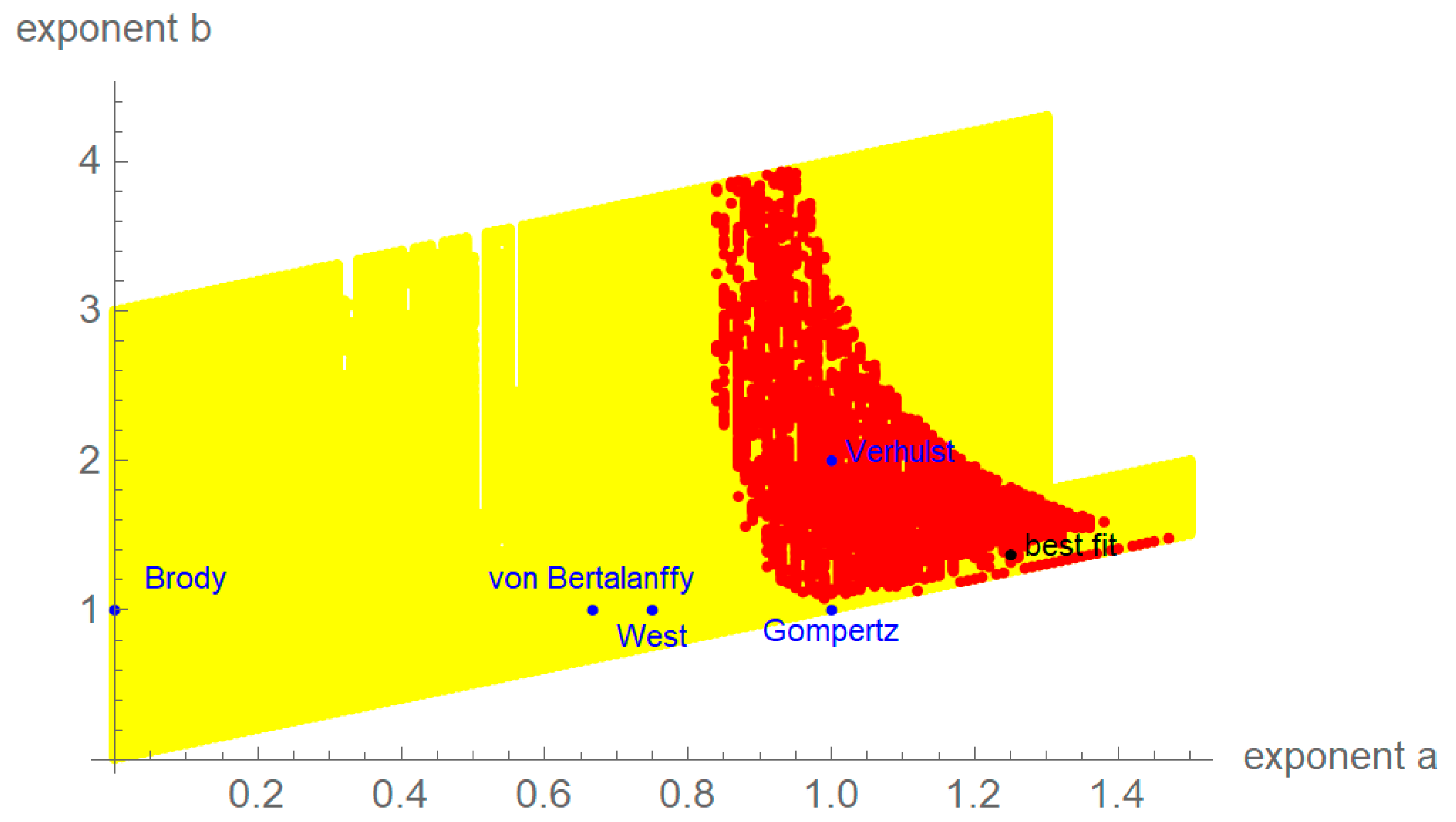
3.2. Best-Fit Exponent Pairs

Several authors have modeled the growth of the car market by the logistic model [5,23]. This model achieved an acceptable fit for all 16 data (R² > 95.21%). The BP models of Table 2 improved the fit significantly. None of the exponent pairs of a named model were close to a best-fit exponent of Table 2; an exception was the Gompertz model (close to electric car GE).

From Table 2, the following pattern emerged that seems to relate the technology of a car to the location of the exponent pair of the best-fitting BP model. The first exponent a was small for gas cars and the difference b–a was low for electric and hybrid cars. Indeed, for three gas car data (natural gas in AT and CH, liquid gas in GE), the first exponent was a = 0 (the growth curve was not sigmoidal). For the fourth gas car data (natural gas in GE), the first exponent was a = 0.01. For the three hybrid car data and for two electric car data, the best-fit exponents were close to the diagonal (b–a = 0.01). For the third electric car data (AT), the difference between the exponents was 0.12. Furthermore, b–a was high for diesel cars; the maximal differences of the exponents (b–a > 2.9) were realized for two diesel data (AT, CH).

The original motivation for the BP model was biological [63]: the exponent pairs characterize certain biophysical situations about the growth of animals [42,43]. While this suggests that the hypothesis that animals of the same species have similar best-fit exponent pairs to describe their growth, in our previous work, we did not find evidence to support this hypothesis. We therefore were surprised by the result of this paper that the best-fit exponents for modeling the growth of the stock of cars from different countries allowed us to distinguish certain drivetrain technologies: gas cars from all three countries were characterized by a small first exponent. Green cars (electric or hybrid) were characterized by a small difference between the exponents.

3.3. Exponent Pairs Leading to Reasonable Fits

Seeking one BP model with a reasonable fit to all data in terms of R-squared, the best choice was BP(0.7, 0.88), with R² > 96.93% for all 16 data; this was a slight improvement over the logistic model. Much better fits were achieved (

Table 5. Models with good fits to all data for certain technologies.

Technology	Good-Fit Model		Comparison of R2 (%)				Alternative
	a	b	Good Fit	Best Fit	Logistic	Alternative	Model
Diesel	0.43	2.07	99.93	99.94	99.58	99.91	West
Petrol	0.36	0.72	99.81	99.82	99.35	99.70
Electric	0.88	0.89	99.56	99.56	99.44	99.53	Gompertz
Hybrid	0.99	1.03	99.50	99.54	99.25	99.47
Gas	0.00	0.58	97.57	97.63	95.12	97.45	Brody

Note: For each technology, the table displays the exponent pair of a good-fit model, so that for each of the data, the minimum of the R² of the good-fit model attains the maximal value shown. This is compared to the minimum of the R² values of the different best-fit models, of the logistic growth model and of an alternative named model, respectively.

) if, for each drivetrain technology, a common model was sought. The reason was antagonism between gas-powered cars and electric or hybrid cars. (To achieve a better fit, for the latter, exponent pairs close to the line a = 0 were needed, while, for the former, the exponent pairs with a better fit were more remote from this line. We observed this antagonism for each country.) The exponent pairs of these models display a similar pattern with respect to the drivetrain technology, as we observed previously for the best-fit exponent pairs. Furthermore, while for nine of the 16 data, an excellent fit of R² > 99.8% could be achieved (Table 2), no single three-parameter BP model achieved this good fit for all nine data. The best outcome was achieved by BP(1.19, 1.2), with R² > 99.8% for seven data.

Furthermore, for different technologies, certain named trend models provided fits that were close to the best achievable fits (Table 5): the Brody model was suitable for gas cars, the Gompertz model (logistic growth was suitable, too) for electric and hybrid cars (this confirms the finding of [36]), and the West model (the Bertalanffy model and logistic growth were suitable, too) for conventional cars (diesel, gasoline). For these models, R-squared was close to the largest R-squared that could be achieved by a single model for all datasets of these classes.

This observation was corroborated by a consideration of the red region in Figure 1 (recomputed for each of the 16 data), indicating likely models. The exponent pair of the Brody model was in the red region for all four gas car data. For the Gompertz model, it was close to the red regions of all six electric and hybrid car data and in addition of three gas car data (from AT and DE). For the West model (and the Bertalanffy model), it was in the red region of two conventional car data (gasoline-AT, diesel-DE) and three gas car data (from AT and DE). For logistic growth, it was in the red region of all electric and hybrid cars (except hybrid-DE).

3.4. Market Dynamics

We applied the BP models to explore the evolution of the market characteristics. We first obtained the best-fit BP models and then we used them to derive the LV Equation (2) for the market evolution. We selected gas cars as the outside goods as, for all countries, this was a rather marginalized drive technology. (For GE, we combined liquid and natural gas cars.) In Austria and Germany, the diesel market shares (computed from the best-fit growth model) decreased during the considered years 2011–2019 and 2012–2019. In Switzerland, diesel shares increased from 2005 to 2013 and decreased from 2013 to 2019. However, the loss of market shares did not necessarily mean a weaker position of diesel cars in terms of the market dynamics. This is because (disregarding the outside good), at the beginning, all technologies in all countries were in a state of competition, i.e., in Equation (2), all coefficients g_i were positive. However, later, a predator–prey dynamic emerged, with diesel cars as the sole prey (g_diesel < 0): this occurred in Germany and Switzerland in 2014 (t = 2.7 and t = 9.8, respectively) and in Austria in 2017 (t = 6.6). Another change occurred in 2018 (t = 13.2) in Switzerland, when gasoline cars became prey, too.

3.5. Did the Diesel Scandal Change the Market Dynamics?

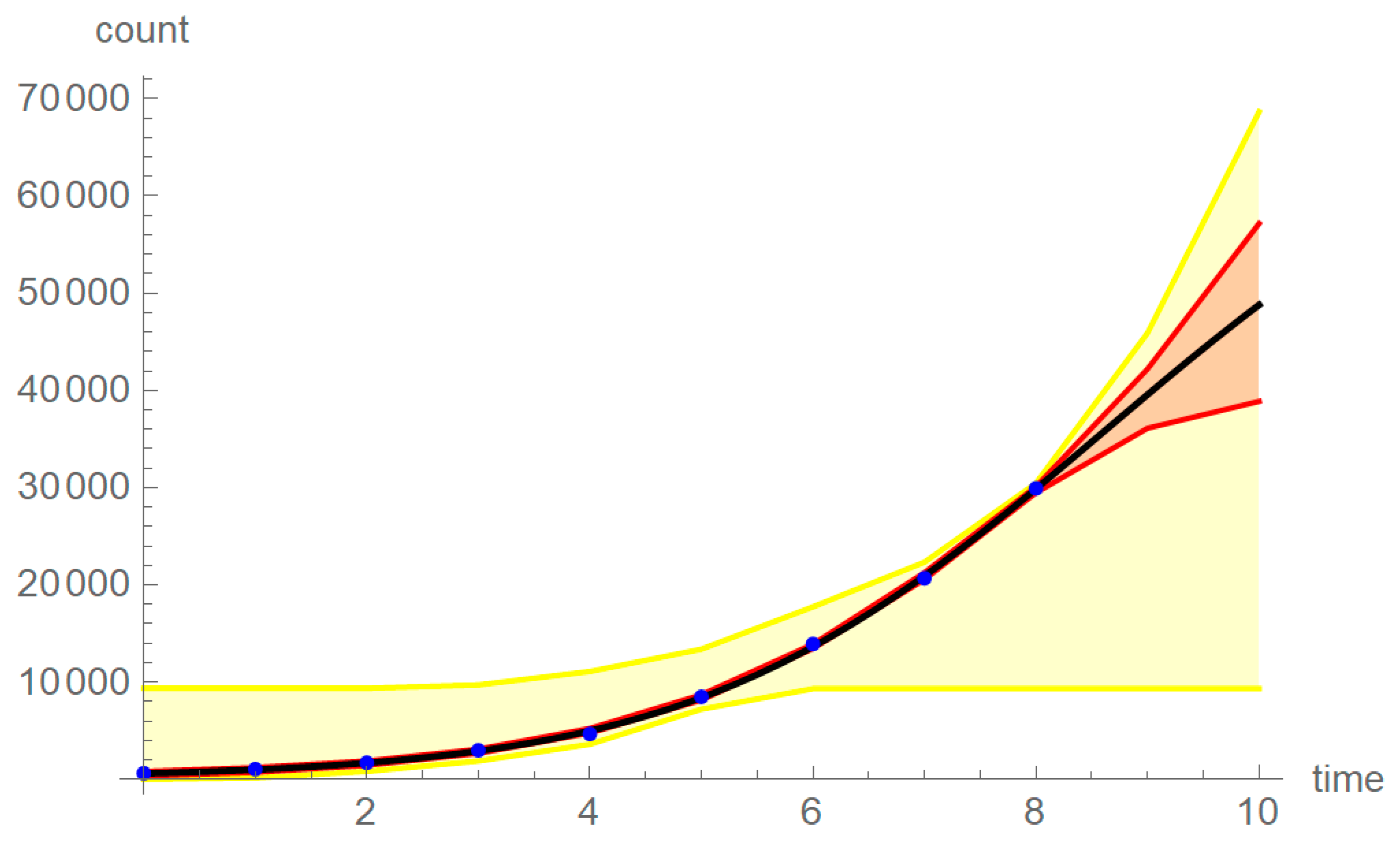
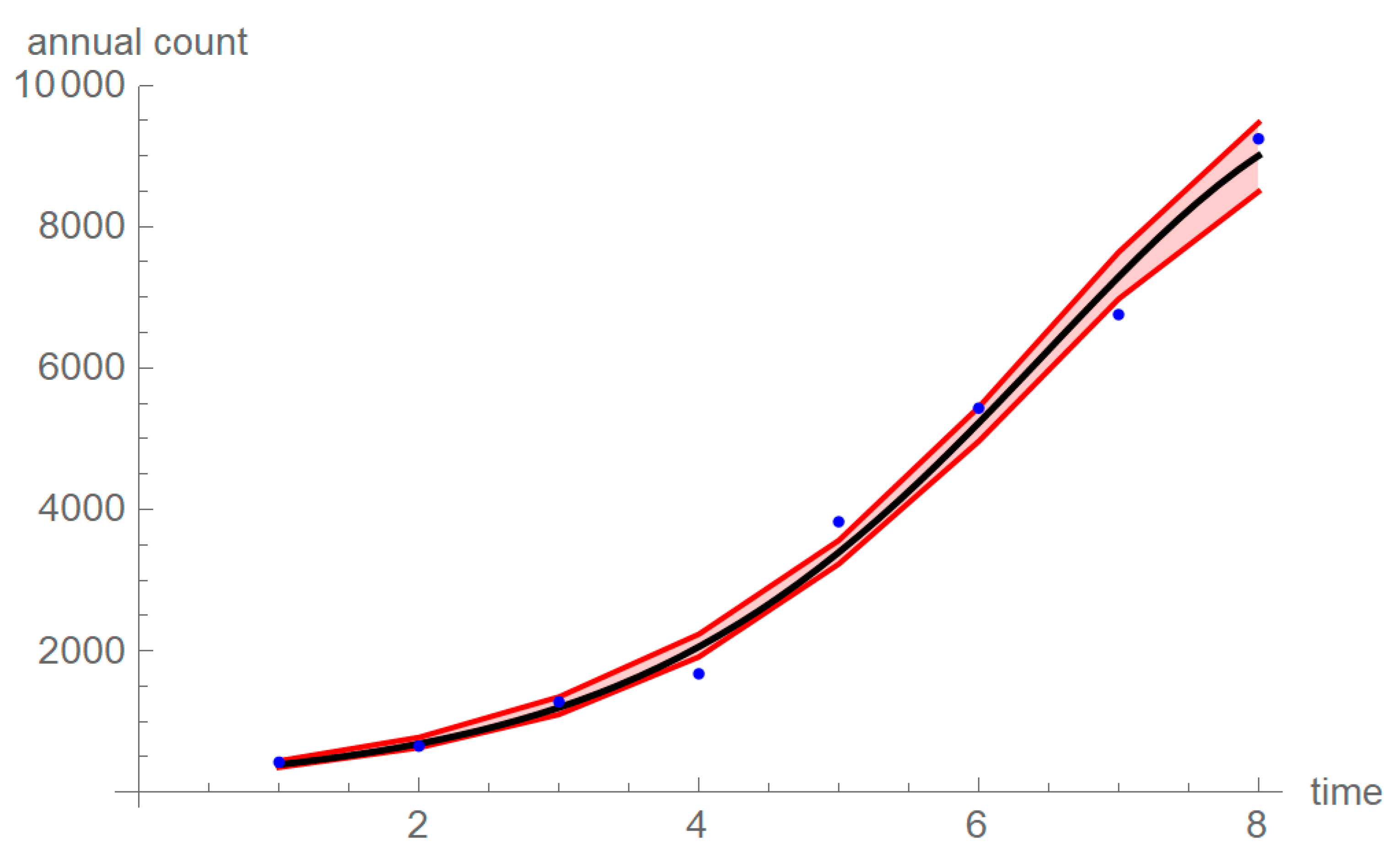
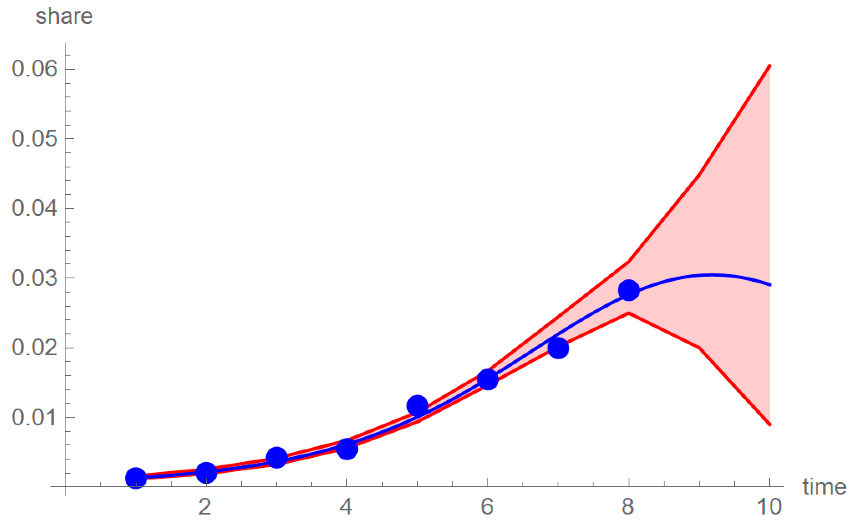
We utilized model uncertainty to arrive at a more differentiated picture of market dynamics in terms of simulations, which augmented the outcomes for the best-fit models with information about other possible scenarios and their likelihood. As follows from our simulations (Table 3), in 2015 (year of the diesel scandal), the market position of diesel cars worsened in Germany and Switzerland. The role of diesel changed from competitor in 2013 and 2014 to (the sole) prey in 2015 and the following years. However, in Austria, other than as suggested by the best-fit models, the market standing of diesel most likely did not worsen, not even in the wake of the diesel scandal.

Table 3 informs about the outcome of the simulations for the years 2013–2021 in more detail: for all countries, the scenario of pair-wise competition was most likely in 2013 and 2014, and the scenario of diesel as the sole prey was most likely for 2015–2019, except for Austria, where pair-wise competition remained the most likely scenario. Thus, for Germany and Switzerland, the simulations suggest that the best-fit model provided a premature date for the change in the role of diesel. However, in view of the high number of simulations with diesel as prey in 2013 (Germany) and 2014 (Germany and Switzerland), it was plausible that, in addition to the diesel scandal, another driver may have supported the change in 2015. Furthermore, other than for the best-fit model, the simulations suggested no change in the competitive pattern for Austria and no additional change after 2015 for Switzerland. Thus, also in this respect, the simulations corrected the best-fit model. This emphasizes the need for an analysis of model uncertainty to supplement the conclusions drawn from best-fit models.

We conclude that the worsening in Germany and Switzerland may not have been caused by the 2015 diesel scandal alone, as, for the simulations, already prior to the scandal, the standing of diesel cars deteriorated. We speculate that also government policies to support environmentally friendly cars by subsidies and privileges (e.g., free parking in cities) may have mattered. Such incentive-based policies [64] have been common for many years in several countries (e.g., Norway, The Netherlands, Sweden) and they were implemented also in Germany [65,66]. However, the VW scandal in turn may have influenced such policy responses, as, e.g., in Germany, it spurred a public debate about the prohibition of conventional cars, which has been recognized in other German-speaking countries as well [67]. Thus, the scandal may have eased the consensus finding in municipal councils for the introduction of disincentives directed specifically against diesel cars. For example, since 2018, the city of Stuttgart, Germany, has enforced a driving ban on old diesel vehicles to reduce air pollution [66]. Similar proposals were considered in Austria and Switzerland.

3.6. Forecasts

From the simulations for 2021, we note that the multi-model approach confirmed that modeling may not be the mathematical equivalent of the “crystal ball”. For all countries, the attempt of a forecast for 2021 remained inconclusive. The simulations resulted in a proliferation of diverse scenarios and, at most, 50% of the simulations resulted in one of the three above-mentioned scenarios (which, in most previous years, accounted for 100%).

The reason is the broadening of the red bands for the extrapolation of the growth functions to the years 2020 and 2021 (as in Figure 2 and Figure 4 for t = 9 and 10). Thus, for the present data, even forecasts for the near future that use likely models only carry significant model uncertainty. For this reason, in this paper, we do not consider forecasting. Furthermore, using trend analysis for this purpose assumes that the past trends will extend into the near future, while unexpected events (e.g., 2020 Covid-19 pandemic) may result in the falsification of such a prognosis.

3.7. Alternative Methodological Approaches

A simple alternative to our approach uses spline interpolation functions s_i(t) of the market shares instead of the BP models. To define the LV model, it uses these splines in Equation (4) to define the coefficients of the LV Equation (2). While this approach reconstructs the market shares without errors, the splines result in complicated utility functions and consequently too many and rather questionable scenarios for the market dynamics (e.g., periods with all market goods in a state of symbiosis, the electric car as the sole predator, the hybrid car as the sole prey). By contrast, the trend analysis of this paper assumes more stability for the consumer preferences.

Our approach resulted in a surprisingly simple shape of the consumer utility functions (f_i of Equation (4); c.f. Figure 5. This leads to the question of whether our modeling approach was overly complex. Why not start with the assumption that utility functions are parabolic in time? One study [68] has proposed this assumption, which leads to a simple alternative route to a LV model for the market shares, explained in Equation (9).

$$\begin{array}{cc}\begin{array}{c}\begin{array}{cc}\begin{array}{cc}{f}_i\left(t\right)=a_i+b_i·t+c_i·t^2& \mathrm{and}\end{array}& z_i\left(t\right)=\frac{\exp \left(f_i\left(t\right)\right)}{1+{{\displaystyle \sum }}_{k\ge 1}\exp \left(f_k\left(t\right)\right)}\end{array}\end{array}& \begin{array}{cc}\mathrm{for}& i\ge 1\end{array}\end{array}$$

(9)

Thereby, z₀ is the remainder of the other z_i to 100%. The starting point is the assumption that the utilities of the market goods are quadratic polynomials. The coefficients (a_i, b_i, c_i) of Equation (9) can be obtained by fitting the polynomial f_i(t) to the observed utilities (they are computed from the observed market shares using formula (3)). Using Equation (9), the solutions z_i of the LV Equation (2) are computed from the utilities [52,53]. Using this approach leads to similar results for the present data. The weaknesses of both approaches are similar, too: as has been illustrated [68] for different data, there may be large fluctuations in the observed market shares around the curves z_i.

An advantage of the present method over the latter approach is the additional information (red band) that can be obtained from the multi-model approach. It allowed us to complement the conclusions from the best-fit model with simulations using models with a nearly best fit. We thereby could refine the market analysis from the best-fit model.

4. Discussion: Outlook on the Open Innovation in the Automotive Industry

The diesel scandal is a case study for the missed chances that arise if industry avoids open innovation. When VW and other companies realized that they could not fulfill the high environmental standards by conventional means (nitrogen oxide storage catalytic converters), they resorted to cheating, thereby exemplifying secrecy mentality at its worst. VW could have avoided this scandal if it had been more open to existing research on innovative technical solutions. For instance, new fuel injection technologies might resolve the pollution problems of diesel engines [69]. Fuel quality might be an issue, too [70]. Samsung is another example of a large corporation whose closed innovation strategy failed [71]: it had to withdraw its “Galaxy Note 7 smartphone” soon after the launch in 2016 (explosion of devices due to deficient batteries).

The resistance to open innovation in large corporations may be due to incompatible management structures [72]. However, there is pressure for a transformation of the traditional automotive industry (see below). As the example of Korean automakers shows, such a transformation of the automotive industry is already under way. They used open innovation in the form of “crowd innovation”, which increased their performance, but at the cost of more patent disputes [73].

For a successful change, first, organizational, cultural, and sometimes also legal barriers need to be removed [74]. Amongst the cultural traits of firms that promote open innovation are a culture of failure acceptance, intra-venturing attitudes and intra-entrepreneurship, and a “transcendental-live firm culture” [75]. Such a culture is generally associated with companies from the information technology sector, e.g., Google or Apple. These are becoming new players in the automotive market, as software-related issues, such as autonomous driving or connected cars, are becoming ever more important [76,77]. Electric vehicles are contributing to this transformation, too. While the production of traditional cars requires high expertise in mechanics, electric cars can be produced by entrepreneurs, e.g., Tesla cars. Still, another pressure for the transformation of automotive industry comes from demands for a circular economy. For example, in 2015, the European Commission set up the action plan “Closing the Loop” [78]. Remanufacturing conventional cars from end-of-life parts saves energy, materials, and costs [79]. In developing countries, several companies specialize in this type of production.

5. Conclusions

We have studied the market diffusion of green cars in three countries. We started with the hypothesis that the diesel scandal might have led to increased sales of electric or hybrid cars. However, our paper has shown that, in the long run, the consumer behavior was surprisingly stable: the diesel scandal alone did not change the market characteristics. In Austria, diesel remained competitive and, in Germany and Switzerland, additional policy measures (prohibitions) were needed to change the consumer behavior, changing diesel from competitor to prey. However, as the car industry is currently undergoing a transformation towards more open innovation, we expect (from analogy to information technology) that the resulting changes from the supply side might create more demand for green cars. However, more research is needed to support this speculation.

References

1. Pathak, K.S.; Sood, V.; Singh, Y.; Channiwala, S.A. Real world vehicle emissions: Their correlation with driving parameters. Transp. Res. Part D 2016, 44, 157–176. [Google Scholar] [CrossRef]
2. Jonson, J.E.; Borken-Kleefeld, J.; Simpson, D.; Nyiri, A.; Posch, M.; Heyes, C. Impact of excess NOx emissions from diesel cars on air quality, public health and eutrophication in Europe. Environ. Res. Lett. 2017, 12. [Google Scholar] [CrossRef] [Green Version]
3. Moshammer, H.; Poteser, M.; Kundi, M.; Lemmerer, K.; Weitensfelder, L.; Wallner, P.; Hutter, H.-P. Nitrogen-dioxide remains a valid air quality indicator. Int. J. Environ. Res. Public Health 2020, 17, 3733. [Google Scholar] [CrossRef] [PubMed]
4. Jansson, J.; Pettersson, T.; Mannberg, A.; Brännlund, R.; Lindgren, U. Adoption of alternative fuel vehicles: Influence from neighbors, family, and coworkers. Transp. Res. Part D 2017, 54, 61–73. [Google Scholar] [CrossRef]
5. Sun, S.; Wang, W. Analysis on the market evolution of new energy vehicle based on population competition model. Transp. Res. Part D 2018, 65, 36–50. [Google Scholar] [CrossRef]
6. Meyer, G.; Müller, B.; Briec, E.; Mazal, C. European Roadmap Electrification of Road Transport. 2012. Available online: https://www.researchgate.net/publication/322625576 (accessed on 10 June 2020).
7. Meyer, G.; Bucknall, R.; Breuil, D. Electrification of the Transport System; European Commission: Brussels, Belgium, 2017. [Google Scholar]
8. Johnson, K.G.E.; Mollenhauer, K.; Tschöke, H. Handbook of Diesel Engines; Springer Science & Business Media: Berlin, Germany, 2010. [Google Scholar]
9. Davenport, C.; Hakim, D. U.S. Sues Volkswagen for Cheating on Emissions Tests. 2016. Available online: https://www.nytimes.com/2016/01/05/business/vw-sued-justice-department-emissions-scandal.html (accessed on 10 June 2020).
10. Mansouri, N. A case study of volkswagen unethical practice in diesel emission test. Int. J. Sci. Eng. Appl. 2016, 5, 211–216. [Google Scholar] [CrossRef]
11. Hayes, R.E.; Mukadi, L.S.; Votsmeier, M.; Gieshoff, J. Three-way catalytic converter modelling with detailed kinetics and washcoat diffusion. Top. Catal. 2004, 30, 411–415. [Google Scholar] [CrossRef]
12. Strittmatter, A.; Lechner, M. Sorting on the used-car market after the Volkswagen emission scandal. J. Environ. Econ. Manag. 2020, 101, 1–41. [Google Scholar] [CrossRef] [Green Version]
13. An, Q.; Christensen, M.G.; Ramachandran, A.; Mukkamala, R.R.; Vatrapu, R. Volkswagen’s diesel emission scandal: Analysis of Facebook engagement and financial outcomes. In Proceedings of the Big Data, 7th International Congress, Held as Part of the Services Conference Federation, Seattle, WA, USA, 25–30 June 2018; pp. 260–276. [Google Scholar] [CrossRef] [Green Version]
14. Jung, J.C.; Sharon, E. The Volkswagen emissions scandal and its aftermath. Glob. Bus. Organ. Excell. 2019, 38, 6–15. [Google Scholar] [CrossRef]
15. Santana, J.C.C.; Miranda, A.C.; Yamamura, C.L.K.; Silva Filho, S.C.; Tambourgi, E.B.; Lee Ho, L.; Berssaneti, F.T. Effects of air pollution on human health and costs: Current situation in São Paulo, Brazil. Sustainability 2020, 12, 4875. [Google Scholar] [CrossRef]
16. Johnson, E. Cars and ground-level ozone: How do fuels compare? Eur. Transp. Res. Rev. 2017, 9, 47. [Google Scholar] [CrossRef]
17. Brondz, I. To be or not to be …? Part III: Diesel versus electrically powered cars. Voice Publ. 2018, 4, 33–50. [Google Scholar] [CrossRef] [Green Version]
18. Sullivan, J.L.; Baker, R.E.; Boyer, B.A.; Hammerle, R.H.; Kenney, T.E.; Muniz, L.; Wallington, T.J. CO2 emission benefit of diesel (Versus Gasoline) powered vehicles. Environ. Sci. Technol. 2004, 38, 3217–3223. [Google Scholar] [CrossRef] [PubMed] [Green Version]
19. Andersen, O.; Upham, P.; Aall, C. Technological response options after the VW diesel scandal: Implications for engine CO2 emissions. Sustainability 2018, 10, 2313. [Google Scholar] [CrossRef] [Green Version]
20. ACEA. The Automobile Industry Pocket Guide, Brussels. 2016. Available online: www.acea.be/uploads/press_releases_files/POCKET_GUIDE_2015-2016.pdf (accessed on 12 June 2020).
21. Stanwick, P.; Stanwick, S. Volkswagen emissions scandal: The perils of installing illegal software. Int. Rev. Manag. Bus. Res. 2017, 6, 18–24. [Google Scholar]
22. Fu, X.; Zhang, P.; Zhang, J. Forecasting and analyzing internet users of China with Lotka-Volterra model. Asia-Pac. J. Oper. Res. 2017, 34. [Google Scholar] [CrossRef]
23. Nguimkeu, P. A simple selection test between the gompertz and logistic growth models. Technol. Forecast. Soc. Chang. 2014, 88, 98–105. [Google Scholar] [CrossRef]
24. Pütter, A. Studien über physiologische ähnlichkeit. VI. Wachstumsähnlichkeiten. Pflügers Arch. Für Die Gesamte Physiol. Des Menschen Und Der Tiere 1920, 180, 298–340. [Google Scholar] [CrossRef]
25. Statistik Austria. Statistiken: Kraftfahrzeuge Neuzulassungen. 2020. Available online: www.statistik.at (accessed on 4 June 2020).
26. Bundesamt, K. Statistik: Neuzulassungsbarometer. 2020. Available online: www.kba.de (accessed on 4 June 2020).
27. STAT-TAB. Neue Inverkehrsetzungen von Strassenfahrzeugen nach Fahrzeuggruppe, Fahrzeugart. 2020. Available online: www.pxweb.bfs.admin.ch (accessed on 4 June 2020).
28. Sheperd, S.P. A review of system dynamics models applied in transportation. Transp. B 2014, 2, 83–105. [Google Scholar]
29. Akaike, H. A new look at the statistical model identification. Ieee Trans. Autom. Control 1974, 19, 716–723. [Google Scholar] [CrossRef]
30. Ohnishi, S.; Yamakawa, T.; Akamine, T. On the analytical solution for the pütter-bertalanffy growth equation. J. Theor. Biol. 2014, 343, 174–177. [Google Scholar] [CrossRef] [PubMed]
31. Bass, F.M. A new product growth model for consumer durables. Manag. Sci. 1969, 15, 215–227. [Google Scholar] [CrossRef]
32. Decock, K.; Debackere, K.; van Looy, B. Bass re-visited: Quantifying multi-finality. Preprint 2020. [Google Scholar] [CrossRef]
33. Brunner, N.; Kühleitner, M.; Nowak, W.G.; Renner-Martin, K.; Scheicher, K. Comparing growth patterns of three species: Similarities and differences. PLoS ONE 2019, 14, e0224168. [Google Scholar] [CrossRef] [Green Version]
34. Adamuthe, A.C.; Thampi, G.K. Technology forecasting: A case study of computational technologies. Technol. Forecast. Soc. Chang. 2019, 143, 181–189. [Google Scholar] [CrossRef]
35. Dhakal, T. An analytical model on business diffusion. J. Ind. Eng. Manag. Sci. 2018, 2018, 119–128. [Google Scholar] [CrossRef] [Green Version]
36. Ma, L.; Wu, M.; Tian, X.; Zheng, G.; Du, Q.; Wu, T. China’s provincial vehicle ownership forecast and analysis of the causes influencing the trend. Sustainability 2019, 11, 3928. [Google Scholar] [CrossRef] [Green Version]
37. Nagula, M. Forecasting of fuel cell technology in hybrid and electric vehicles using Gompertz growth curve. J. Stat. Manag. Syst. 2016, 19, 73–88. [Google Scholar] [CrossRef]
38. Chatzikomis, C.I.; Spentzas, K.N.; Mamalis, A.G. Environmental and economic effects of widespread introduction of electric vehicles in Greece. Eur. Transp. Res. Rev. 2014, 6, 365–376. [Google Scholar] [CrossRef]
39. Verhulst, P.F. Notice sur la loi que la population suit dans son accroissement. Curr. Math. Phys. 1838, 10, 113–121. [Google Scholar]
40. Brody, S. Bioenergetics and Growth; Hafner Publishing Company: New York, NY, USA, 1945. [Google Scholar]
41. Bertalanffy, L.V. Untersuchungen über die Gesetzlichkeit des Wachstums. I. Allgemeine grundlagen der theorie; mathematische und physiologische gesetzlichkeiten des wachstums bei wassertieren. Arch. Für Entwickl. 1934, 131, 613–652. [Google Scholar] [CrossRef]
42. Bertalanffy, L.V. Quantitative laws in metabolism and growth. Q. Rev. Biol. 1957, 32, 217–231. [Google Scholar] [CrossRef] [PubMed]
43. West, G.B.; Brown, J.H.; Enquist, B.J. A general model for ontogenetic growth. Nature 2001, 413, 628–631. [Google Scholar] [CrossRef] [PubMed]
44. Richards, F.J. A flexible growth function for empirical use. J. Exp. Bot. 1959, 10, 290–300. [Google Scholar] [CrossRef]
45. Gompertz, B. On the nature of the function expressive of the law of human mortality, and on a new mode of determining the value of life contingencies. Philos. Trans. R. Soc. Lond. 1832, 123, 513–585. [Google Scholar]
46. Marusic, M.; Bajzer, Z. Generalized two-parameter equations of growth. J. Math. Anal. Appl. 1993, 179, 446–462. [Google Scholar] [CrossRef]
47. Lotka, A.J. Analytical Theory of Biological Populations; Translation of 1934 and 1939 Publications; Plenum Press: New York, NY, USA, 1988. [Google Scholar]
48. Volterra, V. Variazioni e fluttuazioni del numerod’ individui in specie animali conviventi. Mem. Della R. Accad. Dei Lincei 1926, 6, 31–113. [Google Scholar]
49. Smale, S. On the differential equations of species in competition. J. Math. Biol. 1976, 3, 5–7. [Google Scholar] [CrossRef]
50. Modis, T. Genetic re-engineering of corporations. Technol. Forecast. Soc. Chang. 1997, 56, 107–118. [Google Scholar] [CrossRef] [Green Version]
51. Modis, T. Technological forecasting at the stock market. Technol. Forecast. Soc. Chang. 1999, 62, 173–202. [Google Scholar] [CrossRef] [Green Version]
52. Marasco, A.; Picucci, A.; Romano, A. Market share dynamics using Lotka-Volterra models. Technol. Forecast. Soc. Chang. 2016, 105, 49–62. [Google Scholar] [CrossRef]
53. Romano, A. Turning the coin: A competition model to evaluate mergers. J. Res. Ind. Organ. 2013, 443935. [Google Scholar] [CrossRef] [Green Version]
54. Nevo, A.; Rossi, F. An approach for extending dynamic models to settings with multi-product firms. Econ. Lett. 2008, 100, 49–52. [Google Scholar] [CrossRef] [Green Version]
55. Romano, A. A study of tourism dynamics in three italian regions using a nonautonomous integrable lotka–volterra model. PLoS ONE 2016, 11. [Google Scholar] [CrossRef] [Green Version]
56. Marasco, A.; Romano, A. Inter-port interactions in the le Havre-Hamburg range: A scenario analysis using a nonautonomous Lotka Volterra model. J. Transp. Geogr. 2018, 69, 207–220. [Google Scholar] [CrossRef]
57. Lorenčič, V.; Twrdy, E.; Batista, M. Development of competitive-cooperative relationships among mediterranean cruise ports since 2000. J. Mar. Sci. Eng. 2020, 8, 374. [Google Scholar] [CrossRef]
58. Zhang, G.; McAdams, D.A.; Shankar, V.; Darani, M. M Modeling the evolution of system technology performance when component and system technology performances interact: Commensalism and amensalism. Technol. Forecast. Soc. Chang. 2017, 125, 116–124. [Google Scholar] [CrossRef]
59. Loibel, S.; Andrade, M.G.; do Val, J.B.R.; de Freitas, A.R. Richards growth model and viability indicators for populations subject to interventions. An. Acad. Bras. Ciências 2010, 82. [Google Scholar] [CrossRef] [Green Version]
60. Vidal, R.V.V. Applied simulated annealing. In Lecture Notes in Economics and Mathematical Systems; Springer: Berlin/Heidelberg, Germany, 1993. [Google Scholar]
61. Renner-Martin, K.; Brunner, N.; Kühleitner, M.; Nowak, W.G.; Scheicher, K. Best-fitting growth curves of the von bertalanffy-pütter type. Poult. Sci. 2019, 98, 3587–3592. [Google Scholar]
62. Burnham, K.P.; Anderson, D.R. Multi-model inference. Understanding AIC and BIC in model selection. Sociol. Methods Res. 2004, 33, 261–304. [Google Scholar] [CrossRef]
63. Berg, H.A.V.D. Inceptions of biomathematics from Lotka to Thom. Sci. Prog. 2017, 100, 45–62. [Google Scholar] [CrossRef]
64. Bühne, J.; Gruschwitz, D.; Hölscher, J.; Klötzke, M.; Kugler, U.; Schimecek, C. How to promote electromobility for European car drivers? Obstacles to overcome for a broad market penetration. Eur. Transp. Res. Rev. 2015, 7. [Google Scholar] [CrossRef] [Green Version]
65. Langbroek, J.H.M.; Franklin, J.P.; Susilo, Y.O. The effect of policy incentives on electric vehicle adoption. Energy Policy 2016, 94, 94–103. [Google Scholar] [CrossRef]
66. Letmathe, P.; Suares, M. Understanding the impact that potential driving bans on conventional vehicles and the total cost of ownership have on electric vehicle choice in Germany. Sustain. Futures 2020, 2, 100018. [Google Scholar] [CrossRef]
67. Brand, C. Beyond ‘dieselgate’: Implications of unaccounted and future air pollutant emissions and energy use for cars in the United Kingdom. Energy Policy 2016, 97, 1–12. [Google Scholar] [CrossRef] [Green Version]
68. Horgan, D.C. Modelling market share in the UK grocery retail sector using the nonautonomous lotka-volterra equations. Preprint 2020. [Google Scholar] [CrossRef]
69. Pham, V.V.; Cao, D.T. A brief review of technology solutions on fuel injection system of Diesel engine to increase the power and reduce environmental pollution. J. Mech. Eng. Res. Dev. 2019, 42, 1–9. [Google Scholar]
70. Hirota, K.; Kashima, S. How are automobile fuel quality standards guaranteed? Evidence from indonesia, malaysia and vietnam. Transp. Res. Interdiscip. Perspect. 2020, 4. [Google Scholar] [CrossRef]
71. Yun, J.J.; Jeon, J.; Park, K.; Zhao, X. Benefits and costs of closed innovation strategy: Analysis of Samsung’s galaxy note 7 explosion and withdrawal scandal. J. Open Innov Technol. Mark. Complex. 2018, 4, 20. [Google Scholar] [CrossRef] [Green Version]
72. Chiaroni, D.; Chiesa, V.; Frattini, F. Unravelling the process from closed to open innovation: Evidence from mature, asset-intensive industries. RD Manag. 2010, 40, 222–245. [Google Scholar] [CrossRef]
73. Yun, J.J.; Jeong, E.; Zhao, X.; Hahm, S.D.; Kim, K. Collective intelligence: An emerging world in open innovation. Sustainability 2019, 11, 4495. [Google Scholar] [CrossRef] [Green Version]
74. Yun, J.J.; Zhao, X.; Jung, K.; Yigitcanlar, T. The culture for open innovation dynamics. Sustainability 2020, 12, 76. [Google Scholar] [CrossRef]
75. Yun, J.J.; Lee, M.; Park, K.; Zhao, X. Open innovation and serial entrepreneurs. Sustainability 2019, 11, 55. [Google Scholar] [CrossRef] [Green Version]
76. Kim, J.; Chun, M.S.; Nhung, D.T.H.; Lee, J. The transition of samsung electronics through its M&A with harman international. J. Open Innov. Technol. Mark. Complex. 2019, 5, 51. [Google Scholar] [CrossRef] [Green Version]
77. Kodama, F. Incessant conceptual/industrial transformation of automobiles. J. Open Innov. Technol. Mark. Complex. 2019, 5, 50. [Google Scholar] [CrossRef] [Green Version]
78. Hysa, E.; Kruja, A.; Rehman, N.U.; Laurenti, R. Circular economy innovation and environmental sustainability impact on economic growth: An integrated model for sustainable development. Sustainability 2020, 12, 4831. [Google Scholar] [CrossRef]
79. Misran, M.F.R.; Roslin, E.N.; Mohd Nur, N. AHP-consensus judgement on transitional decision-making: With a discussion on the relation towards open innovation. J. Open Innov. Technol. Mark. Complex. 2020, 6, 63. [Google Scholar] [CrossRef]
Figure 1. Exponent pairs as proxy for models. Note: search grid (yellow), exponent pairs with Akaike weight 5% or higher (red), best-fit exponent pair (black), and exponent pairs of selected named models (blue). Plot using Mathematica 12.1 based on the stock of electric cars in Austria (accumulated registration data computed from Table 1).
Joitmc 06 00067 g001
Figure 2. Stock of electric cars in Austria during 2011–2019. Note: stock data (blue dots), best-fit growth curve (black) with the best-fit exponents of Table 2, band of growth curves with an Akaike weight of 5% or higher (red), and band of the best-fit growth curves using any exponent pair from the search grid (yellow); plot using Mathematica 12.1.
Joitmc 06 00067 g002
Figure 3. Annual registrations of electric cars in Austria from 2012 to 2019. Note: blue dots are the registrations (sales) xt, the black line is the derivative y′(tts) of the best-fit curve from Figure 2, using a time shift ts = 0.5, and the red band restricts the range of the derivatives of growth curves with red exponent pairs (Figure 1); plot using Mathematica 12.1.
Joitmc 06 00067 g003
Figure 4. Market shares of electric cars in Austria from 2012 to 2019. Note: blue dots are market share data, the blue line is estimate from Equation (2), using the curve from Figure 3, and the red band restricts the range of the derivatives of the growth curves red exponent pairs (Figure 1); plot using Mathematica 12.1.
Joitmc 06 00067 g004
Figure 5. Utility for electric cars in Austria from 2012 to 2019. Note: utility function computed from the best-fit BP model (blue line) and red band describing the range of the utilities derived from other growth curves with an Akaike weight of 5% or higher; plot using Mathematica 12.1.
Joitmc 06 00067 g005