
Level Structure and Properties of Open f-Shell Elements


1
Helmholtz-Institut Jena, Fröbelstieg 3, D-07743 Jena, Germany
2
GSI Helmholtzzentrum für Schwerionenforschung, D-64291 Darmstadt, Germany
3
Theoretisch-Physikalisches Institut, Friedrich-Schiller-Universität Jena, D-07743 Jena, Germany
Atoms 2022, 10(1), 7; https://0-doi-org.brum.beds.ac.uk/10.3390/atoms10010007
Submission received: 25 November 2021
/
Revised: 31 December 2021
/
Accepted: 1 January 2022
/
Published: 12 January 2022
(This article belongs to the Special Issue Atomic Structure of the Heaviest Elements)
Abstract
:Open f-shell elements still constitute a great challenge for atomic theory owing to their (very) rich fine-structure and strong correlations among the valence-shell electrons. For these medium and heavy elements, many atomic properties are sensitive to the correlated motion of electrons and, hence, require large-scale computations in order to deal consistently with all relativistic, correlation and rearrangement contributions to the electron density. Often, different concepts and notations need to be combined for just classifying the low-lying level structure of these elements. With Jac, the Jena Atomic Calculator, we here provide a toolbox that helps to explore and deal with such elements with open d- and f-shell structures. Based on Dirac’s equation, Jac is suitable for almost all atoms and ions across the periodic table. As an example, we demonstrate how reasonably accurate computations can be performed for the low-lying level structure, transition probabilities and lifetimes for Th ions with a ground configuration. Other, and more complex, shell structures are supported as well, though often for a trade-off between the size and accuracy of the computations. Owing to its simple use, however, Jac supports both quick estimates and detailed case studies on open d- or f-shell elements.
1. Demands of Open -Shell Elements
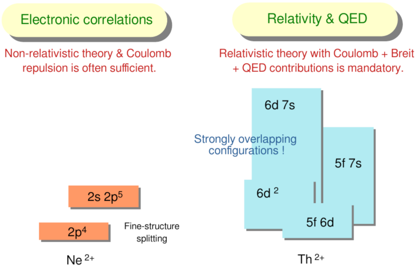
The difficulties in calculating open f-shell elements have long been underrated in atomic theory. Apart from (i) strong relativistic and quantum-electrodynamical (QED) contributions to the level structure in all medium and heavy elements [1,2], difficulties arise especially from (ii) the nearly-degenerate and overlapping configurations, beside the spectroscopic nominated one, as well as (iii) the large number of electrons. All these difficulties have to be taken into account in ab-initio computations for explaining the low-lying levels of such elements. Therefore, the excitation energies and properties of open f-shell elements are not (yet) well understood, even if quite large computations have become feasible today. Figure 1 shows a simple man’s view upon the fine-structure of open-shell elements with its overlapping configurations and strong relativistic contributions [3]. In particular, the actinides are known to exhibit very complex spectra owing to the presence of the open and shells whose fine-structure can be resolved only by high-resolution laboratory studies [4,5,6].
Laser spectroscopy on the (near) optical spectra of actinides has lead to renewed interest in the and elements. Especially, the resonance ionization spectroscopy (RIS) helped greatly improve the knowledge of the low-lying levels and absorption spectra of these heavy elements and to establish highly selective two-step laser excitation schemes [7,8,9]. For example, Chhetri and coworkers [10] applied laser spectroscopy on an atom-at-a-time scale in order to probe the optical spectrum of neutral nobelium with a ground configuration near to its ionization threshold. Indeed, these and similar measurements [11,12,13] paved the way for high-precision spectroscopy of the atomic properties of heavy elements and also provide benchmarks for atomic computations, which include many-body, relativistic and QED contributions at an equal footing.
While laser spectroscopy offers great precision ∼, it usually requires prior knowledge about the level structure and the allowed transitions among the low-lying levels [14]. Until the present, most of these theoretical estimates are typically based on the configuration interaction (CI) or multiconfiguration Hartree-Dirac-Fock (MCDHF) methods, and which help incorporate all major contributions into the electronic structure calculations. When compared with the techniques from (relativistic) many-body perturbation theory (MBPT) [15,16] or coupled-cluster (CC) theory [17], these multi-configurational expansions are conceptional much simpler, especially if electrons occur in—either one or even several—open shells [18]. Successful multi-configuration calculations have been performed for selected low-lying levels of atomic fermium (,14,19]), nobelium [20], lawrencium [21,22] and copernicium [23], aside of a good number of much simpler calculations in the 1980s and 1990s [24,25,26]. For example, neutral fermium has a ground-state and, because of the open f-shell, already a quite detailed fine-structure for just this single configuration. For similar elements with just one or two electrons (or holes) outside of closed shells, more advanced computations have been performed recently also in the framework of relativistic MBPT [27], its combination with fast CI methods [28] as well as by applying the relativistic Fock-space [29] or CC theory [30], to name just a few.
Beyond the level energies, the MCDHF method has been found versatile for dealing also with a rather wide range of atomic processes [18,31,32]. Despite of the frequent application of lanthanides and actinides in photonics, lighting industry or medical research, however, only a few limited tools are available to estimate or calculate the level structure and properties of these elements to good order. For the lanthanides, moreover, radiative transitions were observed in different solutions and doped crystals [33,34], and their emission spectra likely play a relevant role also for developing the next generation light sources for EUV lithography [35].
To fill the gap in dealing with open d- and f-shell elements, we recently developed Jac, the Jena Atomic Calculator [36], which help calculate the level structure and properties as well as a good number of excitation and decay processes for open-shell atoms and ions across the periodic table. This code aims to establish a general and easy-to-use toolbox for the atomic physics community. Below, we shall demonstrate how Jac can be applied to perform both, quick estimations as well as elaborate computations on the representation and properties of these elements. Indeed, a toolbox like Jac need to be developed (further) before the properties of open d- and f-shell elements can be studied with an accuracy comparable to that of simpler shell structures.
To set the background for these tools, the next section first provides a brief account on the theory of the MCDHF method with focus upon the d- and f-shell elements. Apart from the Hamiltonian and wave function expansion, this includes a short overview of Jac and its domain-specific language, the transformation of atomic levels into a coupling scheme as well as the computation of atomic level properties and processes. As an example, we then calculate in Section 3 the low-lying level structure, transition probabilities and lifetimes of Th as widely discussed for developing a nuclear clock; for instance, see Ref. [37]. A few conclusions are finally given in Section 4.
2. Theory and Computations
2.1. Approximate Level Energies and Atomic State Functions
For open d- and f-shell elements, even the levels of the ground configuration can often not be described without that further configurations, nearby in their mean energy, are explicitly included into the representation of the approximate atomic states functions (ASF). In the MCDHF method, these ASF are typically written as superposition of symmetry-adopted configuration state functions (CSF) with well-defined parity P, total angular momentum J and projection M [18],
and where refers to all additional quantum numbers that are needed in order to specify the (N-electron) CSF uniquely. In most standard computations, the set of CSF are constructed as antisymmetrized products of a common set of orthonormal (one-electron) orbitals. In the expansion (1), moreover, the notation has been introduced to just specify an (individual) level symmetry below by its total angular momentum and parity.
In the MCDHF method, the orbitals as well as expansion coefficients are typically both optimized on the Dirac-Coulomb Hamiltonian [2]
in which the one-electron Dirac operator
describes the kinetic energy of the electron and its interaction with the nuclear potential , and where the interaction among the electrons is given by the static Coulomb repulsion . For heavy elements, however, the pairwise interaction between the electrons is often better described by the sum of this Coulomb term and the (so-called) transverse Breit interaction ,
in order to account for the relativistic motion of the electrons. Typically, the Breit interaction is taken in its frequency-independent form as appropriate for most practical computations. For medium and heavy elements, furthermore, the decision about the particular form of the Hamiltonian, that is, of applying either the Dirac-Coulomb operator (2) or the Dirac-Coulomb-Breit operator , or any other approximation to the electron-electron interaction, is usually based upon physical arguments, such as the nuclear charge, the charge state of the ion or the shell structure of interest. In the Jac toolbox, the form of the Hamiltonian and the size of the wave function expansion can be specified quite flexibly in order to account for the relevant relativistic contributions in the representation of the ASF. While we shall refer the reader to the literature for all further details on relativistic atomic structure theory [1,2], let us mention especially the quasi-spin formalism that has been found crucial for systematically-enlarged MCDHF studies on open d- and f-shell elements [38], and which enables one to include single, double and (sometimes even) triple excitations into the wave function expansion (1). This feature is in fact relevant for most heavy and super-heavy () elements, and for which virtual excitations into subshells are often inevitable.
Various proposals have been made in the literature to also incorporate the radiative, or (so-called) QED, corrections in terms of model potentials into the correlated many-electron methods, such as the MCDHF, many-body perturbation or coupled-cluster theories. Following the work by Shabaev et al. [39], these QED corrections can be taken into account by means of a (non-) local single-electron QED Hamiltonian
that comprises effective self-energy (SE) and vacuum-polarization (VP) terms, and that can be treated like local operators. When compared to missing electronic correlations, these QED corrections are often less relevant as long as no inner-shell excitations are involved in any computed property or process [20,40]. For open d- and f-shell elements, indeed, these QED corrections are then considered to be negligible, at least at the present level of computational accuracy, though the CI computations in Jac can be carried out with and without including these QED estimates into the Hamiltonian matrix [41].
2.2. Configuration-Interaction Expansions for Open f-Shell Elements
Ansatz (1) seemingly provides an easy and straightforward way to the generation of atomic bound states. In practice, however, neither the choice of the Hamiltonian nor the construction of the CSF basis turns out to be as simple. For the sake of stability, moreover, the (relativistic) wave functions need often to be optimized layer-by-layer, that is, based on a set of active orbitals with the same principal quantum number n and a predefined maximum ℓ value. By starting from a given list of reference configurations, the wave function expansions are then generated by including single, double, or even triple excitations into ansatz (1). A quite similar concept is realized within the Jac toolbox [36] by means of a configuration-interaction (CI) representation; cf. the data type AtomicState.CiExpansion below. To specify such a representation of the many-electron wave function, use is made of different classes of excitations with regard to the given references and by just stipulating the set of active orbitals. Since all open d- and f-shell elements share quite complex shell structures, only a very limited number of active shells are typically feasible but concede a quick access to the relevant configurations. In general, the costs of ab-initio methods increases hereby very rapidly with the number of active electrons, at least until the open shells are half-filled.
2.3. The Jac Toolbox
2.3.1. Brief Overview of Jac
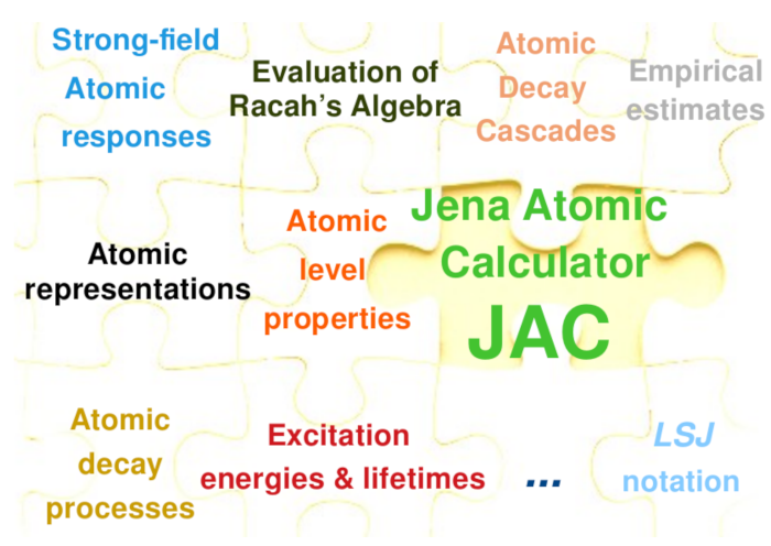
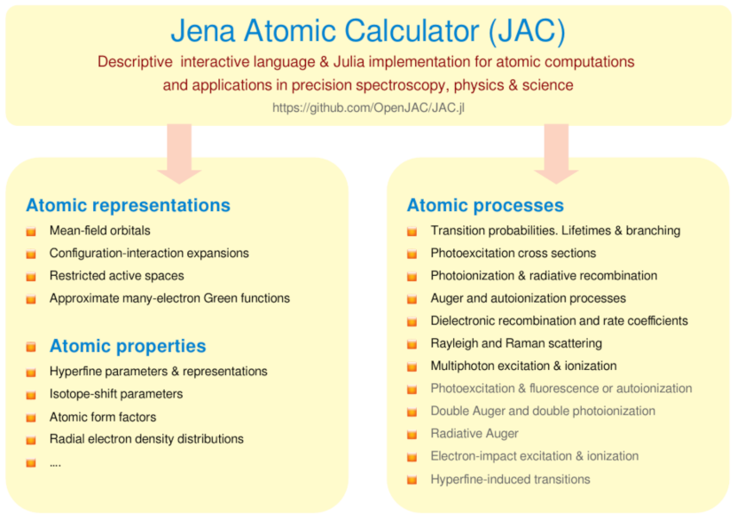
The Jac toolbox has been developed for calculating (atomic many-electron) interaction amplitudes, properties as well as a good number of excitation, ionization and capture processes for open-shell atoms and ions. This toolbox is based on the Dirac-Coulomb (-Breit) Hamiltonian and MCDHF method as briefly outline above. Figure 2 exposes the central features of this program and how it helps integrate different atomic processes within a single computational toolbox in order to ensure good self-consistency of all generated data. Jac is implemented in Julia, a new programming language for scientific computing, and which is known to include a number of (modern) features, such as dynamic types, optional type annotations, type-specializing, just-in-time compilation of code, dynamic code loading as well as garbage collection [42,43].
Little need to be said about the design of Jac that has been described elsewhere [36,41] and can readily be downloaded from the web [44]. This toolbox can be utilized without much prior knowledge of the code. One of Jac’s rather frequently applied kind of computation for medium and heavy elements refers to the (so-called) Atomic.Computations. These computation are based on explicitly specified electron configurations and (help) provide level energies, the representation of ASF or selected level properties. They also help evaluate the transition amplitudes (and rates) as the numerical key for predicting the fluorescence spectra and lifetimes of the low-lying excited levels. Below, we shall explain and discuss how this toolbox can be employed in order to estimate the level energies and lifetimes for the low-lying levels of Th. For many (standard) computations, indeed, Jac provides an interface which is equally accessible for researchers from experiment, theory as well as for code developers. Jac’s careful design enables the user to gradually approach different applications of atomic theory.
The Jac toolbox is internally built upon (the concept of) many-electron amplitudes that generally combine two atomic bound states of the same or of two different charge states, and may thus include free electrons in the continuum [45]. These amplitudes are then employed to compute the—radiative and nonradiative—rates, lifetimes or cross sections as shown below. Advantage of these tools is taken also to formulate (and implement) atomic cascade computations in a language that remains close to the formal theory [46,47]. The consequent use of these amplitudes is quite in contrast to most other atomic structure codes that are based on some further decomposition of these (many-electron) amplitudes into various one- and two-particle (reduced) matrix elements, or even into radial integrals, well before any coding is done.
2.3.2. Needs of a Descriptive Language for Atomic Computations
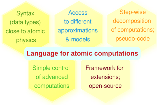
During the past decades, the demands to atomic structure and collision theory have changed distinctly from the accurate computation of a few low-lying level energies and properties towards (massive) applications in astro, plasma and technical physics, and at several places elsewhere. These demands make it desirable to develop a domain-specific and descriptive language, for instance built upon Julia, which not only reveal the underlying formalism but also avoids most technical details. Apart from a concise syntax, close to the formulation of atomic physics problems, such a domain-specific language should support access to different models and approximations as well as the decomposition of a given task into well-designed steps, similar to writing pseudo-code. Figure 3 points out several requirements for such a language of doing atomic physics, and for which Jac aims for. These requirements appear quite opposite to most previous—either Fortran or C—codes, for which simple extensions, a rapid proto-typing or the use of graphical interfaces often becomes cumbersome. Aside of these rather practical demands, such a language should as well support a transparent communication with and within the code, independent of the shell structure of the atoms or any particular application. For performing quantum many-particle computations, moreover, the language must be fast and flexible enough in order to implement all necessary building blocks. By using Julia with its deliberate language design, we therefore hope to bring over productivity and performance also to the Jac toolbox.
2.3.3. Combining Syntax and Semantics: Jac’s Data Structures for Atomic Computations
Julia’s type system is known as one of its strongest features, when compared with many other computing languages [42]. In Julia, all types are said to be first-class and are utilized to select the code dynamically by means of (so-called) multiple dispatch. While abstract data types are used to establish a hierarchy of relationships between data and actions, and are applied in order to model behavior, the actual data are always kept by concrete types, either as primitive and composite types. Moreover, abstract and concrete types can be both parametric to further enhance the dynamic code allocation. All these rather general concepts are also well adopted in Jac to facilitate the communication with as well as the data transfer within the program. In fact, the Jac toolbox is built upon ∼250 such properly designed data structures. These structures define many useful and frequently recurring objects in order to deal with the level energies and processes of atoms and ions, and to make the implementation rather independent from the particular shell structure. Obviously, in addition, the (notion of most of these) data types should be readily understandable to any atomic physicist without much additional training. A few prominent examples of these data types are an Orbital to represent the quantum numbers and radial components of (one-electron) orbital functions, an atomic Basis to specify a set of CSF, or a Level for the full representation of a single ASF: as shown in expansion (1). Frankly speaking, these data structures form the basic language elements in order to specify and describe the desired computations.
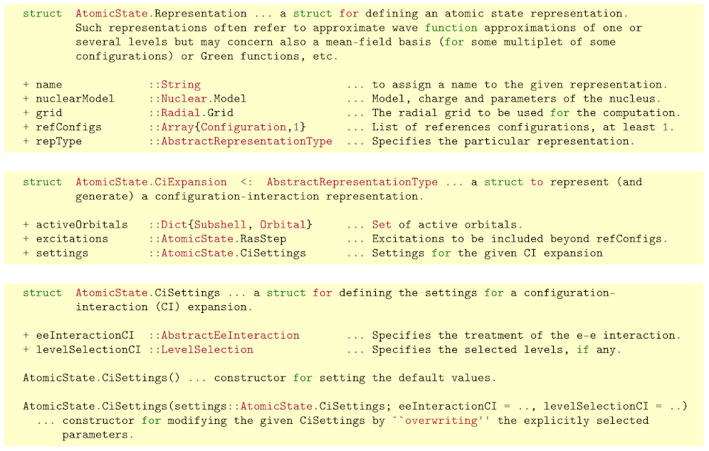
While most of Jac’s data types (may) remain hidden to the user, this set typically needs to be enlarged in order to implement and explore new applications. Table 1 lists a few of these data types for predicting the properties of open d- and f-shell elements. For example, the AtomicState.Representation and its subtype AtomicState.CiExpansion have been found to be crucial to generate well-designed CI expansions for the computation of level energies and properties [48]. Figure 4 displays the definition of these data types together with the CiSettings in order to control the set of active orbitals and virtual excitation. Other wave function representations, which are partly supported by the Jac toolbox, refer to a MeanFieldBasis for generating a mean-field basis and a set of orbitals, a RasExpansion for dealing with restricted active-space (RAS) wave functions or a GreenExpansion for computing an approximate (many-electron) Green function [49]. These representations are subtypes of the AbstractRepresentationType from the same module. Although not all details of these data types will be explained here, Figure 4 shows how the data are communicated and maintained within the Jac program. Each representation and process (see below) usually comes with its own Settings in order to facilitate the detailed control of all computations, even if the default values are typically sufficient. Obviously, however, the careful design of these data types help keep the computations feasible.
2.4. Spectroscopic Notation for Open f-Shell Elements
Since relativistic computations are regularly based on -coupling, a (unitary) transformation need first to be carried out for determining the notation of the levels as usually applied in atomic spectroscopy. In Jac, such a transformation can be performed optionally for all or a selected number of levels. This is achieved by fixing LSjjSettings(true) in the AsfSettings as associated with any self-consistent-field computation for the wave functions of a given multiplet. Apart from the level assignment of the multiplet, Jac also supports a full transformation of the wave functions from a - to a -coupled basis by just setting the minWeight parameter to zero in the LSjjSettings. For open d- and f-shell elements, however, such a complete unitary transformation matrix is of little help and often results in just lengthy computations.
For open d- and f-shell atoms, a level notation is often needed already for classifying even the lowest part of the level structure owing to the very rich fine-structure. Indeed, the lack of providing a fast and proper spectroscopic notation in relativistic computations have hindered the spectroscopic level classification of heavy elements and the analysis of their (inner-shell) processes. If we formally express the wave function expansion (1) of atomic levels as [51,52]:
in the - and -coupled basis, the nonrelativistic Fourier coefficients are implemented in Jac for up to two (nonrelativistic) open shells. Internally, this re-expansion of the -coupled levels into a basis makes use of the shell-dependent overlap integrals [53] as previously implemented already within the Ratip code [32]. Below, we shall discuss how this transformation can be utilized in order to classify the low-lying level structure of Th ions.
2.5. Atomic Amplitudes and Properties
As mentioned before, the many-electron amplitudes between either CSF or approximate ASF are central to any implementation in atomic (structure) theory, from the set-up of the Hamiltonian matrix to the interaction of the electrons with the nuclear moments (hyperfine structure), to autoionization and electron capture processes, and up to the coupling of atoms to the radiation field. In Jac, three of these amplitudes refer to the electron–electron interaction, the multipole-moment and transition amplitudes as well as the momentum-transfer amplitudes, which can all be invoked by the user, if the atomic states (levels) and operators are properly specified. From these and a few other amplitudes, the fine and hyperfine splitting [54], isotope shifts [55,56], Lande factors, atomic form factors, level-dependent fluorescence yields, or several other properties can be readily derived. Figure 5 displays selected applications of the Jac toolbox for predicting the properties and processes of atoms and ions, though not all of these processes have yet been implemented in full detail (as indicated by gray color).
The properties above can be examined by means of Atomic.Computations, a key data type of Jac that enables the user to describe the problem in sufficient detail. These computations are based on the levels (multiplets) as obtained from a set of configurations. Two examples for such computations will be shown below for the low-lying level structure of Th.
While atomic units are used throughout for all internal computations, the input and output of Jac is based on user-specified units, which can be overwritten interactively. The current (default) settings of the units are displayed on screen by typing Basics.display(“settings”), and they can readily be modified by Defaults.setDefaults(), if the default settings are not appropriate. For example, the call Defaults.setDefaults(“unit: energy”, “Kayser”) or Defaults.setDefaults(“unit: energy”, “Hartree”) tells Jac that all further inputs and outputs are handled either in Kaysers or Hartrees (atomic units), if not stated otherwise.
2.6. Atomic Excitation and Decay Processes of Open f-Shell Elements
Today, several implementations of the MCDHF method support correlated expansions (1) also for open d- and f-shell elements. These approximate bound states can then be applied for obtaining the cross sections and rates of different atomic processes. In fact, a good number of such processes are known in atomic and plasma physics, including various excitation, ionization, recombination and scattering processes. Until the present, however, processes with—one or a few—electrons in the continuum still remain as a challenge for atomic theory, and this applies especially if atoms with open valence-shell structures are involved. Apart from the bare number of amplitudes and channels, difficulties in dealing with free electrons arise in particular from the rearrangement of the electron density, if the initial and final states are well separated in energy or simply belong to different charge states. Table 2 just lists a few of these processes; all of these computations can again be carried out by means of Atomic.Computations. Moreover, since each of these properties and processes is implemented by a separate module, this number can be readily enlarged in the future if needs arise from the user side.
3. Low-Lying Level Structure of Th
Computations of the electronic structure and properties of free atoms and ions have been found a powerful tool to explore the interaction of matter with light and particles of various kinds as well as in different—physical and chemical—environments. For open d- and f-shell atoms and ions, however, only a few ab-initio case studies exist because of the difficulties mentioned in the introduction. Accurate Fock-space and CC calculations have been carried out especially for the low-lying levels of selected atoms with just one or two electrons (or holes) outside of closed-shells. For most other lanthanide and actinide elements, in contrast, either restricted multiconfigurational calculations [25] have been performed or very little is still known at all until now. With the Jac toolbox, we wish to overcome these limitations and to facilitate—medium to large-scale—ab-initio computations also for these medium and heavy elements. Although further work is needed to make the code efficient, the variety of atomic level properties and processes, so far implemented in Jac, will support the spectroscopy of open d- and f-shell elements in the future, including the actinides. In this section, we therefore show how the low-lying level energies and lifetimes can (at least) be estimated.
3.1. Estimates on the Level Structure of Th
Th ions still have a simple odd-parity ground configuration with a ground-state level. However, the low-lying even-parity configurations are nearby in energy and give rise to a level just 63 cm above of the ground state. For six even-parity levels of the and configurations at UV excitation energies, moreover, Biemont et al. [57] measured the lifetimes by using the time-resolved laser-induced fluorescence method. From observing the lines of Th and other radio-active ions, the age of individual stars has been estimated in the Milky Way. At present, the NIST database [58] list 200 low-lying levels of Th, and to which we shall compare our computations below, though many of these levels are still unknown or not yet fully identified.
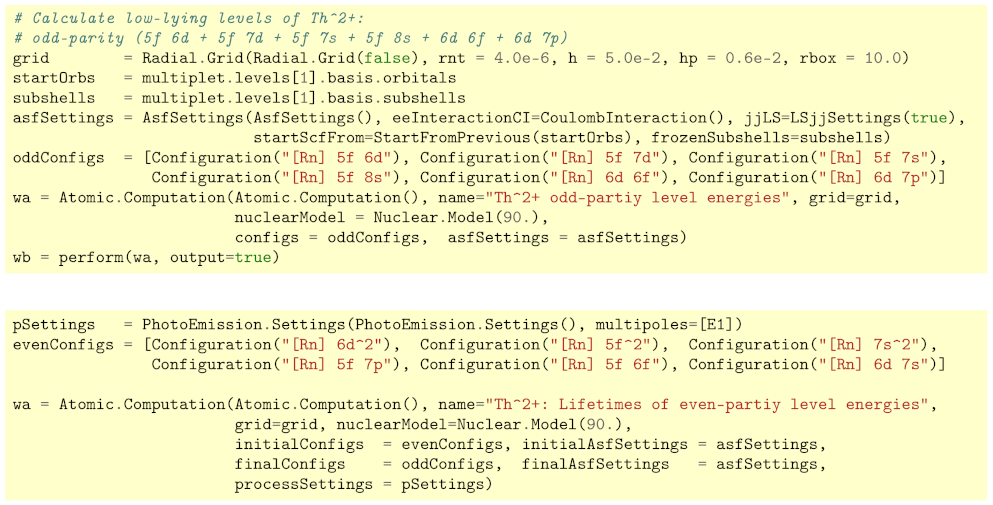
To demonstrate the easy use of the Jac toolbox, we here consider the level structure of the odd-parity and even-parity configurations. For the odd-parity levels, Figure 6 displays the input for Jac that needs to be compiled prior to the computations. Apart from specifying a suitable radial grid and nuclear model, we need to provide the necessary configurations, and where just refers to the radon ground configuration. By re-specifying some fields of the default AsfSettings(), we furthermore tell the program to restrict the electron–electron interaction in the CI computations to the Coulomb repulsion [cf. Equation (2)] and to request for a transformation of all levels of interest. Indeed, this is all input that need to be provided to an Atomic.Computation in order to overwrite the default settings as obtained by the plain constructor Atomic.Computation(). Many more details could be specified but are omitted here for the sake of simplicity. Once an Atomic.Computation has been specified with just the essential physical information, that is, all the details to make the computational task explicit, it should be simply performed in order to return the results either tabulated or in a graphical form. Because of the complexity of open d- and f-shell elements, all other steps are then carried out automatically, making use of some default values. These steps especially refer to the computation of a self-consistent field, the setup and diagonalization of the Hamiltonian matrix based on the Dirac–Coulomb (–Breit) operator and, if requested, to the calculation of further transition amplitudes and probabilities. Since, moreover, we have demanded a transformation of all calculated levels in Figure 6, we also obtain the leading notation of these levels, together with their weights within the given representation.
Table 3 displays the excitation energies as obtained from the Atomic.Computation above. Results are shown for the 16 low-lying odd-parity levels with total angular momentum . These excitation energies can be compared with experiments [58,59] and the calculations by Safronova et al. [60], who combined the configuration-interaction and linearized coupled-cluster methods. These excitation energies agree within ∼2000 cm with the NIST tabulations, although larger deviations may occur for several highly-exited and even-parity levels. These deviations can be attributed to the rather limited set of active orbitals in the present computations. For the high-lying levels, indeed, the identification is typically less easy and requires the knowledge of the leading notations. To improve these energies, we could either include further configurations explicitly in the Atomic.Computation above or perform a more advanced AtomicState.RasExpansion. Such a restricted active space (RAS) expansion applies, analogous to a CI expansion, a user-specified excitation scheme to a given set of reference configurations in order to generate the requested configurations automatically and, hence, to ensure a systematic enlargement of the given basis. These RAS expansions are usually generated stepwise since, more often than not, the correlation orbitals need to be frozen before the next layer of orbitals can be optimized in addition to the pre-determined charge distribution. In practice, however, such RAS expansions are (much) less useful for open d- and f-shell elements because of their rich fine-structure. Some further gain in efficiency can be achieved by dividing the CSF basis into groups of CSF with the same symmetry , and where the rearrangement of the electron density retains partly included in the computation for levels of different symmetry.
While Figure 6 shows perhaps a surprisingly simple input to calculate and analyze the fine-structure of Th ions, this “simplicity” becomes relevant especially if other open f-shell ions or their properties and processes need to be considered. Apart from the standard input, the user has extensive control about the interatomic interactions and the amount of correlations, if the defaults are carefully overwritten.
3.2. Transition Probabilities. Lifetimes and Branching Fractions
For open f-shell elements, the transition probabilities and lifetimes need often to be estimated in order to identify and characterize the low-lying level structure from the intensities of the observed line spectra. In Jac, such estimates can readily be done by just modifying a few lines in the input as shown in the lower panel of Figure 6.
Here, the (value of the) processSettings tells Jac to calculate the Einstein A and B coefficients as well as the oscillator strength for the photon emission from the even- to odd-parity levels, and as associated with the initial- and final-state configurations. In these computations, we just consider—in line with the defaults of the Jac toolbox—the electric-dipole transitions, although these defaults can also be readily modified within the code. Once the Atomic.Computation has been performed, all results are usually tabulated in a neat format, both at screen and within a summary file. In these tables, the atomic levels and transitions are then listed in terms of the level numbers as they arise from the diagonalization of the associated Hamiltonian matrix within the Jac program [32,40]. Moreover, the (full) representation of the initial and final-state multiplets as well as all the computed transition data can be obtained eventually if the optional argument output=true is given to the function perform(). Since the initial and final-state multiplets are determined independently in the computation of all atomic processes, the rearrangement of the electron density is partly taken into account, though no attempt has been made so far to deal with this non-orthogonality in the evaluation of the angular coefficients.
We shall not display and compare here explicitly the transition probabilities with previous computations, and with typically a better agreement for the strong than the weak transitions. However, Table 3 compares the lifetime estimates from the present computations with the measurements by Biemont et al. [57] and recent calculations [60]. For these even parity levels with energies ≳32,000 cm, both the energies and lifetimes still exhibit rather large uncertainties due to the limited configuration basis of the present computations. Again, the identification of these levels is possible by means of a transformation and the analysis of the leading terms. The lifetimes are shown here in velocity gauge and were found to differ by up to a factor of 3 from the corresponding length-gauge computations. Since we wish to demonstrated the simple use of the Jac toolbox, no further enlargement is shown for the wave-function expansion nor the derived properties. Our two examples however manifest how Jac can be employed to generate much larger surveys of fine-structure levels as well as the—radiative and nonradiative—decay branches of the resonantly excited ion.
4. Summary and Conclusions
While the difficulties with open d- and f-shell elements can hardly be overrated, we have shown how the Jac toolbox is utilized to perform reasonably accurate computations for these shell structures. In particular, we explain how these tools help estimate the energies and properties for complex fine-structures. Apart from such simple estimates, Jac can also be applied to approximate and systematically improve relativistic ASF by including different classes (schemes) of virtual excitations with regard to a given set of reference configurations. In addition, the Jac toolbox also facilitates the computation of atomic processes, cascades or even the symbolic simplification of expressions from Racah’s algebra [61].
Numerical results are shown above for the low-lying level structure of Th ions. These and similar computations for other actinide ions will be useful for developing new excitation schemes for heavy elements and for applications in medicine, radiation safety or elsewhere. Although, at present, the Jac program can often not immediately compete with its (numerical) accuracy with many-body perturbation or all-order techniques; these tools will help to go beyond the currently available applications of relativistic atomic structure theory.
Since Jac’s very first design in 2017, the number of atomic properties and processes that can be handled by this code has grown steadily and it now supports the generation of (atomic) data for astro and plasma physics [62]. In fact, there are at present various demands to further advance the Jac toolbox: For open d- and f-shell elements, these requests mainly refer to efficiency and memory issues, the re-use of angular coefficients or the coupling of free electrons in ionization or capture processes. With the present version, however, a major step has already been made to obtain useful estimates and data for a large class of heavy and super-heavy elements.
Funding
This research received no external funding.
Conflicts of Interest
The author declares no conflict of interest.
References
- Johnson, W.R. Atomic Structure Theory: Lectures on Atomic Physics; Springer: Berlin/Heidelberg, Germany, 2007. [Google Scholar]
- Grant, I.P. Relativistic Quantum Theory of Atoms and Molecules: Theory and Computation; Springer: Berlin/Heidelberg, Germany, 2007. [Google Scholar]
- Fritzsche, S. Large–scale accurate structure calculations for open–shell atoms and ions. Phys. Scr. 2002, T100, 37. [Google Scholar] [CrossRef]
- Raeder, S.; Ackermann, D.; Backe, H.; Block, M.; Cheal, B.; Chhetri, P.; Düllmann, C.E.; van Duppen, P.; Even, J.; Ferrer, R.; et al. Nuclear properties of nobelium isotopes from laser spectroscopy. Phys. Rev. Lett. 2018, 120, 232503. [Google Scholar] [CrossRef] [PubMed] [Green Version]
- Raeder, S.; Kneip, N.; Reich, T.; Studer, D.; Trautmann, N.; Wendt, K. Recent developments in resonance ionization mass spectrometry for ultra-trace analysis of actinide elements. Radiochim. Acta 2019, 107, 1515. [Google Scholar] [CrossRef]
- Rothe, S.; Andreyev, A.N.; Antalic, S.; Borschevsky, A.; Capponi, L.; Cocolios, T.E.; Witte, H.D.; Eliav, E.; Fedorov, D.V.; Fedosseev, V.N.; et al. Measurement of the first ionization potential of astatine by laser ionization. Nat. Commun. 2013, 4, 1835. [Google Scholar] [CrossRef] [Green Version]
- Flanagan, K.T.; Lynch, K.M.; Billowes, J.; Bissell, M.L.; Budincevic, V.; Cocolios, T.E.; de Groote, R.P.; Schepper, S.D.; Fedosseev, V.N.; Franchoo, S.; et al. Collinear resonance ionization spectroscopy of neutron-deficient francium isotopes. Phys. Rev. Lett. 2013, 111, 212501. [Google Scholar] [CrossRef] [PubMed] [Green Version]
- Ferrer, R.; Barzakh, A.; Bastin, B.; Beerwerth, B.; Block, M.; Creemers, P.; Grawe, H.; de Groote, R.; Delahaye, P.; Fléchard, X.; et al. Towards high-resolution laser ionization spectroscopy of the heaviest elements in supersonic gas jet expansion. Nat. Commun. 2017, 8, 14520. [Google Scholar] [CrossRef] [Green Version]
- Granados, C.; Creemers, P.; Ferrer, R.; Gaffney, L.P.; Gins, W.; de Groote, R.; Huyse, M.; Kudryavtsev, Y.; Martnez, Y.; Raeder, S.; et al. In-gas laser ionization and spectroscopy of actinium isotopes near the N=126 closed shell. Phys. Rev. C 2017, 96, 054331. [Google Scholar] [CrossRef] [Green Version]
- Chhetri, P.; Ackermann, D.; Backe, H.; Block, M.; Cheal, B.; Droese, C.; Düllmann, C.E.; Even, J.; Ferrer, R.; Giacoppo, F.; et al. Precision measurement of the first ionization potential of nobelium. Phys. Rev. Lett. 2018, 120, 263003. [Google Scholar] [CrossRef] [PubMed]
- Laatiaoui, M. On the way to unveiling the atomic structure of superheavy elements. Eur. Phys. J. Conf. 2016, 131, 05002. [Google Scholar] [CrossRef] [Green Version]
- Laatiaoui, M.; Buchachenko, A.A.; Viehland, L.A. Exploiting transport properties for the detection of optical pumping in heavy ions. Phys. Rev. A 2020, 102, 013106. [Google Scholar] [CrossRef]
- Sato, T.K.; Asai, M.; Tsukada, K.; Kaneya, Y.; Toyoshima, A.; Mitsukai, A.; Nagame, Y.; Osa, A.; Toyoshima, A.; Tsukada, K.; et al. First ionization potentials of Fm, Md, No, and Lr: Verification of filling-up of 5f electrons and confirmation of the actinide series. J. Am. Chem. Soc. 2018, 140, 14609. [Google Scholar] [CrossRef] [Green Version]
- Sewtz, M.; Backe, H.; Dretzke, A.; Kube, G.; Lauth, W.; Schwamb, P.; Eberhardt, K.; Grüning, C.; Thörle, P.; Trautmann, N.; et al. First observation of atomic levels for the element fermium (Z = 100). Phys. Rev. Lett. 2003, 90, 163002. [Google Scholar] [CrossRef] [Green Version]
- Morrison, J.C.; Rajnak, K. Many-body calculations for the heavy atoms. Phys. Rev. 1971, A4, 536. [Google Scholar] [CrossRef]
- Borschevsky, A.; Pershina, V.; Eliav, E.; Kaldor, U. Ab initio predictions of atomic properties of element 120 and its lighter group-2 homologues. Phys. Rev. A 2013, 87, 022502. [Google Scholar] [CrossRef]
- Eliav, E.; Kaldor, U.; Ishikawa, Y. Transition energies of mercury and ekamercury (element 112) by the relativistic coupled-cluster method. Phys. Rev. 1995, 52, 2765. [Google Scholar] [CrossRef] [PubMed]
- Grant, I.P. Relativistic Effects in Atoms and Molecules. In Methods in Computational Chemistry; Wilson, S., Ed.; Plenum: New York, NY, USA, 1988; Volume 2, pp. 1–38. [Google Scholar]
- Sewtz, M.; Backe, H.; Dong, C.Z.; Dretzke, A.; Eberhardt, K.; Fritzsche, S.; Grüning, C.; Haire, R.G.; Kube, G.; Kunz, P.; et al. Resonance ionization spectroscopy of fermium (Z = 100). Spectrochim. Acta B 2003, 58, 1077. [Google Scholar] [CrossRef]
- Fritzsche, S. On the accuracy of valence–shell computations for heavy and super–heavy elements. Eur. Phys. J. D 2005, 33, 15. [Google Scholar] [CrossRef]
- Zou, Y.; Froese Fischer, C. Resonance transition energies and oscillator strengths in lutetium and lawrencium. Phys. Rev. Lett. 2002, 88, 183001. [Google Scholar] [CrossRef] [PubMed]
- Fritzsche, S.; Dong, C.Z.; Koike, F.; Uvarov, A. The low–ying level structure of atomic lawrencium (Z = 103): Energies and absorption rates. Eur. Phys. J. D 2007, 45, 107. [Google Scholar] [CrossRef]
- Yu, Y.J.; Li, J.G.; Dong, C.Z.; Ding, X.B.; Fritzsche, S.; Fricke, B. The excitation energies, ionization potentials and oscillator strengths of neutral and ionized species of Uub (Z = 112) and the homologue elements Zn, Cd and Hg. Eur. Phys. J. D 2007, 44, 51. [Google Scholar] [CrossRef]
- Fricke, B.; Greiner, W.; Waber, J.T. The continuation of the periodic table up to Z = 172. The chemistry of superheavy elements. Theor. Chim. Acta 1971, 21, 235. [Google Scholar] [CrossRef]
- Johnson, E.; Pershina, V.; Fricke, B. Ionization potentials of Seaborgium. J. Phys. Chem. 1999, 103, 8458. [Google Scholar] [CrossRef]
- Johnson, E.; Fricke, B.; Jacob, T.; Dong, C.Z.; Fritzsche, S.; Pershina, V. Ionization potentials and radii of neutral and ionized species of elements 107 (bohrium) and 108 (hassium) from extended multiconfiguration Dirac-Fock calculations. J. Phys. Chem. 2002, 116, 1862. [Google Scholar] [CrossRef]
- Eliav, E.; Fritzsche, S.; Kaldor, U. Electronic structure theory of the superheavy elements. Nucl. Phys. A 2015, 944, 518. [Google Scholar] [CrossRef]
- Kahl, E.V.; Berengut, J.C.; Laatiaoui, M.; Eliav, E.; Borschevsky, A. High-precision ab initio calculations of the spectrum of Lr+. Phys. Rev. 2019, A100, 062505. [Google Scholar] [CrossRef] [Green Version]
- Oleynichenko, A.V.; Zaitsevskii, A.; Skripnikov, L.V.; Eliav, E. Relativistic Fock space coupled cluster method for many-electron systems: Non-perturbative account for connected triple excitations. Symmetry 2020, 12, 1101. [Google Scholar] [CrossRef]
- Kumar, R.; Chattopadhyay, S.; Angom, D.; Mani, B.K. Relativistic coupled-cluster calculation of the electric dipole polarizability and correlation energy of Cn, Nh+, and Og: Correlation effects from lighter to superheavy elements. Phys. Rev. A 2021, 103, 062803. [Google Scholar] [CrossRef]
- Fritzsche, S.; Surzhykov, A.; Stöhlker, T. Dominance of the Breit interaction in the X-ray emission of highly charged ions following dielectronic recombination. Phys. Rev. Lett. 2009, 103, 113001. [Google Scholar] [CrossRef] [Green Version]
- Fritzsche, S. The Ratip program for relativistic calculations of atomic transition, ionization and recombination properties. Comp. Phys. Commun. 2012, 183, 1525. [Google Scholar] [CrossRef]
- Judd, B.R. Correlation crystal fields for lanthanide ions. Phys. Rev. Lett. 1977, 39, 242. [Google Scholar] [CrossRef]
- Dorenbos, P. Crystal field splitting of lanthanide 4fn-15d levels in inorganic compounds. J. Alloys Comp. 2002, 341, 156. [Google Scholar] [CrossRef]
- Suzuki, C.; Koike, F.; Murakami, I.; Tamura, N.; Sudo, S. Systematic observation of EUV spectra from highly charged lanthanide ions in the large helical device. Atoms 2018, 6, 24. [Google Scholar] [CrossRef] [Green Version]
- Fritzsche, S. A fresh computational approach to atomic structures, processes and cascades. Comp. Phys. Commun. 2019, 240, 1. [Google Scholar] [CrossRef]
- Seiferle, B.; von der Wense, L.; Thirolf, P.G. Lifetime measurement of the 229Th nuclear isomer. Phys. Rev. Lett. 2017, 118, 042501. [Google Scholar] [CrossRef] [Green Version]
- Gaigalas, G.; Fritzsche, S.; Rudzikas, Z. Reduced coefficients of fractional parentage and matrix elements of the tensor W(kqkj) in jj-coupling. At. D. Nucl. D. Tables 2002, 76, 235. [Google Scholar] [CrossRef]
- Shabaev, V.M.; Tupitsyn, I.I.; Yerokhin, V.A. Model operator approach to the Lamb shift calculations in relativistic many-electron atoms. Phys. Rev. A 2013, 88, 012513. [Google Scholar] [CrossRef] [Green Version]
- Indelicato, P.; Santos, J.P.; Boucard, S.; Desclaux, J.-P. QED and relativistic corrections in superheavy elements. Eur. Phys. J. D 2007, 45, 155. [Google Scholar] [CrossRef]
- Fritzsche, S. JAC: User Guide, Compendium & Theoretical Background. Unpublished. Available online: https://github.com/OpenJAC/JAC.jl/blob/master/UserGuide-Jac.pdf (accessed on 10 October 2021).
- Julia 1.7 Documentation. Available online: https://docs.julialang.org/ (accessed on 10 December 2021).
- Bezanson, J.; Chen, J.; Chung, B.; Karpinski, S.; Shah, V.B.; Vitek, J.; Zoubritzky, L. Julia: Dynamism and performance reconciled by design. Proc. ACM Program. Lang. 2018, 2, 120. [Google Scholar] [CrossRef] [Green Version]
- GitHub—OpenJAC / JAC.jl. Available online: https://github.com/OpenJAC/JAC.jl (accessed on 10 November 2021).
- Fritzsche, S.; Fricke, B.; Sepp, W.D. Reduced L1 level-width and Coster-Kronig yields by relaxation and continuum interactions in atomic zinc. Phys. Rev. A 1992, 45, 1465. [Google Scholar] [CrossRef] [PubMed] [Green Version]
- Fritzsche, S.; Palmeri, P.; Schippers, S. Atomic cascade computations. Symmetry 2021, 13, 520. [Google Scholar] [CrossRef]
- Schippers, S.; Martins, M.; Beerwerth, R.; Bari, S.; Holste, K.; Schubert, K.; Viefhaus, J.; Savin, D.W.; Fritzsche, S.; Müller, A. Near L-edge single and multiple photoionization of singly charged iron ions. Astrophys. J. 2017, 849, 5. [Google Scholar] [CrossRef] [Green Version]
- Fritzsche, S.; Froese Fischer, C.; Gaigalas, G. A program for relativistic configuration interaction calculations. Comput. Phys. Commun. 2002, 148, 103. [Google Scholar] [CrossRef]
- Fritzsche, S.; Surzhykov, A. Approximate atomic Green functions. Molecules 2021, 26, 2660. [Google Scholar] [CrossRef] [PubMed]
- Julia Comes with a Full-Featured Interactive and Command-Line REPL (Read-Eval-Print Loop) That Is Built into the Executable of the Language. Available online: https://docs.julialang.org/en/v1/stdlib/REPL/ (accessed on 10 December 2021).
- Gaigalas, G.; Zalandauskas, T.; Fritzsche, S. Spectroscopic LSJ notation for atomic levels as obtained from relativistic calculations. Comput. Phys. Commun. 2004, 157, 239. [Google Scholar] [CrossRef] [Green Version]
- Gaigalas, G.; Fritzsche, S. Angular coefficients for symmetry-adapted configuration states in jj-coupling. Comput. Phys. Commun. 2021, 267, 108086. [Google Scholar] [CrossRef]
- Gaigalas, G.; Fritzsche, S. Maple procedures for the coupling of angular momenta. VI. LS-jj transformations. Comput. Phys. Commun. 2002, 159, 39. [Google Scholar] [CrossRef] [Green Version]
- Fischer, A.; Canali, C.; Warring, U.; Kellerbauer, A.; Fritzsche, S. First optical hyperfine structure measurement in an atomic anion. Phys. Rev. Lett. 2010, 104, 073004. [Google Scholar] [CrossRef]
- Cocolios, T.E.; Dexters, W.; Seliverstov, M.D.; Andreyev, A.N.; Antalic, S.; Barzakh, A.E.; Bastin, B.; Büscher, J.; Darby, I.G.; Fedorov, D.V.; et al. Early onset of ground state deformation in neutron deficient polonium isotopes. Phys. Rev. Lett. 2011, 106, 052503. [Google Scholar] [CrossRef] [Green Version]
- Cheal, B.; Cocolios, T.E.; Fritzsche, S. Laser spectroscopy of radioactive isotopes: Role and limitations of accurate isotope-shift calculations. Phys. Rev. A 2012, 86, 042501. [Google Scholar] [CrossRef]
- Biemont, E.; Palmeri, P.; Quinet, P.; Zhang, Z.G.; Svanberg, S. Doubly ionized thorium: Laser lifetime measurements and transition probability determination of interest in cosmochronology. Astrophys. J. 2002, 567, 1276. [Google Scholar] [CrossRef] [Green Version]
- Kramida, A.; Ralchenko, Y.; Reader, J.; NIST ASD Team. NIST Atomic Spectra Database (ver. 5.8), [Online]. 2021. Available online: https://physics.nist.gov/asd (accessed on 25 October 2021).
- Wyart, J.-F.; Kaufman, V. Extended analysis of doubly ionized thorium (Th III). Phys. Scr. 1981, 24, 941. [Google Scholar] [CrossRef]
- Safronova, M.S.; Safronova, U.I.; Clark, C.W. Relativistic all-order calculations of Th, Th+, and Th2+ atomic properties. Phys. Rev. A 2014, 90, 032512. [Google Scholar] [CrossRef] [Green Version]
- Fritzsche, S. Symbolic evaluation of expressions from Racahs algebra. Symmetry 2021, 13, 1558. [Google Scholar] [CrossRef]
- Fritzsche, S. Dielectronic recombination strengths and plasma rate coefficients of multiply-charged ions. Astron. Astrophys. 2021, 656, A163. [Google Scholar] [CrossRef]
Figure 1.
A simple man’s view of the fine-structure of open-shell atoms and ions. For light elements, such as Ne with a ground configuration, the excitation of a valence-shell electron leads to levels that are energetically well separated, and whose configurations can be treated rather independently. For open d- and f-shell elements, in contrast, many configurations overlap with each other, and this even applies for the ground configuration. While the fine-structure of Ne is well separated by ∼200,000 cm from the configuration, the ground configuration of Th ‘overlaps’ with the fine-structure levels of several and both, odd- and even-parity configurations. For any detailed ab-initio calculations, therefore, electronic correlations as well as relativistic and QED contributions need always to be taken into account for a quite large number of configurations.

Figure 2.
Overview of the Jac toolbox [36] for calculating atomic and ionic structures, processes and cascades, based on Dirac’s equation and the MCDHF method. This toolbox facilitates a variety of relativistic computations as briefly shown in this jigsaw puzzle. In this work, Jac is especially applied to predict the excitation energies and level properties of open d- and f-shell elements.

Figure 3.
Requirements for establishing a domain-specific and descriptive atomic language as is implemented in Jac.
Figure 3.
Requirements for establishing a domain-specific and descriptive atomic language as is implemented in Jac.

Figure 4.
Definition of the data types AtomicState.Representation (upper panel), AtomicState.CiExpansion (middle panel) and AtomicState.CiSettings (lower panel) to select and perform a configuration interaction computation as discussed in the text. CI wave functions utilize a single step of a restricted-active-space (RAS) expansion and the associated virtual excitations that are to be applied with regard to the given reference configurations.

Figure 5.
Selected applications of the Jac toolbox to generate atomic representations or to compute properties and processes. See Refs. [36,41] for a more detailed account of the various features of this toolbox.

Figure 6.
Input for the Atomic.Computation of the low-lying levels of Th. In these calculations (upper panel), the orbitals of the [Rn] configuration have first been optimized independently and then be kept frozen in the computation above. In the (lower panel), in addition, the transition probabilities and lifetimes are obtained by just specifying the even-parity configurations as well as the Settings for the photo emission.


Table 1.
Selected data types of the Jac toolbox for predicting the properties of open d- and f-shell elements. Here, only a brief explanation is given, while further details can be found at Julia’s REPL [50] by typing, for instance, ? Representation.
Table 1.
Selected data types of the Jac toolbox for predicting the properties of open d- and f-shell elements. Here, only a brief explanation is given, while further details can be found at Julia’s REPL [50] by typing, for instance, ? Representation.
| Struct | Brief Explanation |
|---|---|
| AbstractEeInteraction | Abstract type to distinguish between different electron-electron interaction operators; it comprises the concrete (singleton) types BreitInteraction, CoulombInteraction, CoulombBreit. |
| AbstractExcitationScheme | Abstract type to support different excitation schemes, such as DeExciteSingleElectron, ExciteByCapture, and several others. |
| AbstractScField | Abstract type for dealing with different self-consistent-field (SCF) potentials. |
| AsfSettings | Settings to control the SCF and CI calculations for a given multiplet. |
| Atomic.Computation | An atomic computation of one or several multiplets, including the SCF and CI calculations, as well as of selected properties or processes. |
| Basis | (Relativistic) many-electron basis, including the specification of the configuration space and all radial orbitals. |
| Configuration | (Nonrelativistic) electron configuration as specified by the shell occupation. |
| EmMultipole | A multipole (component) of the electro-magnetic field as specified by its electric or magnetic character and the multipolarity. |
| Level | Atomic level in terms of its quantum numbers, symmetry, energy and its (possibly full) representation. |
| LevelSelection | List of levels that is specified by either the level numbers and/or level symmetries. |
| LevelSymmetry | specifies the (total) angular momentum and parity of a particular level. |
| LSjjSettings | Settings to control the transformation of the selected many-electron levels. |
| MeanFieldBasis | A simple representation of the electronic structure in terms of a mean-field orbital basis. |
| Multiplet | An ordered list of atomic levels, often associated with one or several configurations. |
| Nuclear.Model | A model of the nucleus to keep all nuclear parameters together. |
| Orbital | (Relativistic) radial orbital function that appears as building block in order to define the many-electron CSF; such an orbital comprises a large and small component and is typically given on a (radial) grid. |
| Radial.Grid | Radial grid to represent the (radial) orbital function and to perform all radial integration. |
| Radial.Potential | Radial potential function. |
| Representation | Representation of an atomic state in terms of either a mean-field basis, an approximate wave function, a many-electron Green function, or others. |
| RasExpansion | A restricted active-space representation of the levels from a given multiplet; cf. CiExpansion in Figure 3. |
| RasSettings | Settings to control the details of a RasExpansion. |
| RasStep | Single-step of a (systematically enlarged) restricted active-space computation. |
| Shell | Nonrelativistic shell, such as . |
| Subshell | Relativistic subshell, such as |
Table 2.
Selected excitation, capture and decay processes that can be calculated by means of the Jac toolbox. refers to the excitation and to some possible excitation of an atom or ion with regard to its ground configuration.
Table 2.
Selected excitation, capture and decay processes that can be calculated by means of the Jac toolbox. refers to the excitation and to some possible excitation of an atom or ion with regard to its ground configuration.
| Process & Brief Explanation |
|---|
| Photon emission : Transition probabilities; oscillator strengths; lifetimes; angular distributions. |
| Photoexcitation : Excitation cross sections, alignment parameters; statistical tensors. |
| Photoionization : Cross sections; angular parameters. |
| Photorecombination : Recombination cross sections; angular parameters. |
| Auger emission or autoionization : Auger rates; angular and polarization parameters. |
| Dielectronic recombination (DR) : Partial and total DR resonance strengths; DR plasma rate coefficients. |
| Photoexcitation with subsequent autoionization : Rates. |
| Photo-double ionization : Energy-differential and total cross sections. |
| Rayleigh & Compton scattering of light : Angle-differential cross sections. |
Table 3.
Excitation energies [eV] and lifetimes [s] of Th. Data from the Jac toolbox are compared with the NIST database ([58]), experiments and previous computations. Results are shown for 16 low-lying levels. These energetically low-lying levels can be identified uniquely using their energy and total symmetry despite of certain level crossings. In general, strong admixtures of other symmetries are typically found for these levels, which increase further as the valence-shell structure is “opened” further. See text for discussion.
| Level | Energy [eV] | Lifetime [s] | ||||||
|---|---|---|---|---|---|---|---|---|
| This Work | Exp. [58] | Calc. [60] | This Work | Exp. [57] | Calc. [60] | |||
| 0 | 0 | 0 | ||||||
| 210 | 511 | 189 | ||||||
| 3686 | 2527 | 2436 | ||||||
| 4975 | 3182 | 2958 | ||||||
| 3026 | 3188 | 3207 | ||||||
| 5360 | 4827 | 4853 | ||||||
| 4863 | 4490 | 4802 | ||||||
| 6857 | 5060 | 5085 | ||||||
| 8466 | 6288 | 5797 | ||||||
| 6702 | 6311 | 6237 | ||||||
| 9279 | 7501 | 7609 | ||||||
| 8779 | 7921 | 8260 | ||||||
| 9192 | 8142 | 8197 | ||||||
| 8555 | 8437 | 8810 | ||||||
| 13,084 | 11,123 | 11,564 | ||||||
| 15,274 | 11,233 | 11,766 | ||||||
| 37,134 | 32,867 | 33,488 | [−8] | [−8] | [−8] | |||
| 43,256 | 38,581 | 38,980 | [−8] | [−9] | [−9] | |||
| 46,404 | 42,260 | - | [−9] | [−9] | [−9] | |||
| 47623 | 45,064 | - | [−9] | [−9] | [−9] | |||
| 55,884 | 53,052 | - | [−9] | [−9] | [−9] | |||
Publisher’s Note: MDPI stays neutral with regard to jurisdictional claims in published maps and institutional affiliations. |
© 2022 by the author. Licensee MDPI, Basel, Switzerland. This article is an open access article distributed under the terms and conditions of the Creative Commons Attribution (CC BY) license (https://creativecommons.org/licenses/by/4.0/).
Share and Cite
MDPI and ACS Style
Fritzsche, S. Level Structure and Properties of Open f-Shell Elements. Atoms 2022, 10, 7. https://0-doi-org.brum.beds.ac.uk/10.3390/atoms10010007
AMA Style
Fritzsche S. Level Structure and Properties of Open f-Shell Elements. Atoms. 2022; 10(1):7. https://0-doi-org.brum.beds.ac.uk/10.3390/atoms10010007
Chicago/Turabian StyleFritzsche, Stephan. 2022. "Level Structure and Properties of Open f-Shell Elements" Atoms 10, no. 1: 7. https://0-doi-org.brum.beds.ac.uk/10.3390/atoms10010007
Note that from the first issue of 2016, this journal uses article numbers instead of page numbers. See further details here.