Effects of the FEL Fluctuations on the 2s2p Li⁺ Auto-Ionization Lineshape

Abstract

The photoionization of Lithium (Li${}^{+}$) via its doubly-excited state 2s2p ${}^{1}P$ in intense free electron laser (FEL) radiation is studied. A recently developed perturbative statistical description of the atomic dynamics is used to calculate the ionization yield. It is observed that the FEL temporal fluctuations affect the lineshape significantly, strongly dependent on the product of the pulse’s coherence time with its intensity, $\sim {\tau }_c{I}_0$, which is a measure of the effect of the field in one correlation time. The weak-field long-pulse asymmetric resonant Fano-profile is broadened to resemble a Voight profile. As the intensity increases, the subsequent ionization of Li${}^{2+}$ takes over and causes further distortion of the lineshape for Li${}^{+}$.

1. Introduction

The advent of high-order harmonic generation (HOHG) and Free-Electron Laser (FEL) sources in the last two decades has made available radiation which is sufficiently short to compete with sub-femtosecond atomic characteristic times and sufficiently intense to compare and surpass the static interatomic electric fields by orders of magnitudes [1,2,3,4,5]. An important characteristic of this radiation is that it can spatially penetrate the interior of atomic-size systems and interact with the innermost electrons directly; a property which is in complete contrast with intense, long-wavelength, laser (i.e., Ti:Sapphire) where the outermost electrons act as a shield and disallow probe of the inner regions even if the necessary energy is available in the form of multiphoton absroptions. A natural consequence of these breakthrough developments is a shift of the interest to explore and control the dynamics of atomic systems in the short-wavelength radiation regime [1,2,3,6,7,8].

In the case of ionization with FEL sources very often the measurements of observables are taken after the target systems have interacted many times with pulses which differ each other in random ways (multishot experiments); then the experimental reports provide only statistically averaged values of the observables. For this class of experiments it is inevitable that the temporal fluctuations in the atomic photoionization dynamics should be properly taken into account, in principle, for a fair comparison with the experimental data. This simple fact brings at the forefront a statistical description of the atomic dynamics and in fact there are already a number of works where various theoretical approaches have been applied [9,10,11,12].

Recently, we took the effort to develop a perturbative statistical theory which provides the equations-of-motion for the atomic dynamical observables of theoretical and experimental interest (excited population, ionization yield, electron kinetic/angular spectrum, absorption spectrum, etc.) [12]. More specifically we treated the near-resonant photoionization processes as stochastic processes characterized by the fluctuation statistics of the FEL radiation. The FEL was modelled as non-stationary Gaussian stochastic field in line with the model developed by Krinsky and Li [13]; within this model the FEL statistics has its origin in the self-amplified spontaneous emission (SASE) start-up process, which in turn is treated as a shot-noise stochastic process [14,15,16].

In the present work we investigate the lineshape of the ionization of Li${}^{+}$ for FEL fields in the proximity of the $2s2p^{1}P$ autioinization resonance (AIS). The calculation is based on (a) an ab-initio calculation of the electronic structure and the AIS parameters (position and width of the resonance) [17,18,19,20] (b) a formulation of the density matrix elements time-evolution in the Fano basis states (EOMs) [21] (c) the elimination of the continuum state dynamics as well as the subsequent average of the EOMs [12]. Here we do not repeat all the necessary details of the calculations but rather present those steps that are relevant with the particular application to Li${}^{+}$.

In Section 2 we discuss the calculation method for the atomic structure and the way we extract the Fano parameters from the knowledge of the photoionization cross section and the position and width of the AIS. In Section 3, we present the EOMs for the density matrix elements of the system and in Section 4 their averaged form is presented for the case of a Gaussian, non-stationary FEL field. Finally in Section 5 we investigate the effects of the fluctuations on the lineshape of the ionization yield.

For the presentation of the formulas, atomic units (a.u.) are used throughout the text; For the reader’s convenience other units (e.g., eV, fs) are used in the discussion section and the figures caption.

2. Electronic Structure and the Fano Picture of Resonant Ionization

As mentioned, a detailed exposition of the method is included in References [19,20]. Nevertheless, in order to present the logical flow of the calculations we will briefly give the steps involved here; the calculation of the electronic structure [19], the derivation of the density matrix equations [21] and their stochastic average [12] as these are adapted in the present work.

2.1. Atomic Structure Calculations

First we describe the method followed to calculate the transition amplitudes involved in the photoionization process. The Li${}^{+}$ Hamiltonian in atomic units is given by,

$${\widehat{H}}_a({\mathit{r}}_1,{\mathit{r}}_2)=\sum _{i=1,2}\widehat{h}\left({\mathit{r}}_i\right)+\widehat{V}({\mathit{r}}_1,{\mathit{r}}_2)=\sum _{i=1}^2(-\frac{1}{2}{\overrightarrow{\nabla }}_i^2-\frac{3}{r_i})+\frac{1}{r_{12}},$$

(1)

where the one-electron Hamiltonians $\widehat{h}\left({\mathit{r}}_i\right)$ and the interelectronic potential, $\widehat{V}({\mathit{r}}_1,{\mathit{r}}_2)$ are defined by inspection.

We consider the interaction of the Li${}^{+}$ with FEL radiation. Within the non-relativistic approximation a proper Hilbert space to develop a formulation is the one generated by the eigenstates of the total energy, square of the angular momentum and spin operators as well as the corresponding projections, namely, ${\widehat{H}}_a,{\widehat{L}}^2,{\widehat{S}}^2,{\widehat{L}}_z,{\widehat{S}}_z$, where $\widehat{L}={\widehat{l}}_1+{\widehat{l}}_2$, $\widehat{S}={\widehat{s}}_1+{\widehat{s}}_2$, where ${\widehat{l}}_i,{\widehat{s}}_i$ are the angular momenta and spin quantum numbers of the two-electrons. Since the interaction between the Li${}^{+}$ and the FEL radiation does not contain any spin operators and assuming the electric field linearly polarized along the $z–$axis the projection of the total angular momentum and the spin quantum numbers are invariants of the ionization process; which means that the possible states reached, following interaction with the FEL, are singlet states with the same total magnetic quantum number as the ground state, $|g\rangle =|1s^2{,}^{1}S\rangle$. So in the below all states have $L_z=0$ and $S=0,M_S=0$. The eigenstates are denoted by $|nL\rangle$, the first index representing the eigenenergy, E, and the second one the angular momentum L, values

Having defined the basis, the aim now is the numerical calculation of the two-electron eigenstates of the above Hamiltonian. To this end, the eigenvalue problem to be solved is,

$${\widehat{H}}_a{\Phi }_{E_{n}L}({\mathit{r}}_{\mathbf{1}},{\mathit{r}}_{\mathbf{2}})=E_{nL}{\Phi }_{E_{n}L}({\mathit{r}}_{\mathbf{1}},{\mathit{r}}_{\mathbf{2}}),$$

(2)

where ${\Phi }_{E_{n}L}({\mathit{r}}_{\mathbf{1}},{\mathit{r}}_{\mathbf{2}})$ are the eigenstates of ${\widehat{H}}_a$ (two-electron field free wavefunctions). The system is assumed to be confined in a sphere of radius R, much larger than the atomic size dimensions. The solution of the partial differential Equation (2) requires the boundary condition to be set, which in our case is to have the wavefunction vanish at the origin and at the boundary, R. Consequently all eigenstates (including the continuum) are now discrete and the bound and continuum states are treated on equal footing. A configuration interaction (CI) approach is employed where the eigenstates are expanded on an uncorrelated two-electron basis ${\varphi }_{n_1{l}_1{n}_2{l}_2}^L({\mathit{r}}_{\mathbf{1}},{\mathit{r}}_{\mathbf{2}})$, formed by Slater determinants of angular momentum coupled one-electron states (configurations) found from the one-electron TISE. More specifically the uncorrelated two-electron basis functions are the eigensolutions of the zero-order Hamiltonian, ${\widehat{H}}_a^{\left(0\right)}={\widehat{h}}_1\left({\mathit{r}}_1\right)+{\widehat{h}}_2\left({\mathit{r}}_2\right)$, with eigenstates,

$${\varphi }_{n_1{l}_1{n}_2{l}_2}^L({\mathit{r}}_{\mathbf{1}},{\mathit{r}}_{\mathbf{2}})=A_{12}\frac{P_{n_1{l}_1}\left(r_1\right)}{r_1}\frac{P_{n_2{l}_2}\left(r_2\right)}{r_2}{\mathcal{Y}}_{l_1{l}_2}^{L0}({\Omega }_1,{\Omega }_2),$$

(3)

where ${\mathcal{Y}}_{l_1{l}_2}^{L{M}_L=0}({\Omega }_1,{\Omega }_2)$ are the bipolar spherical harmonics, containing the angular momentum coupling coefficients (Clebsch-Gordon coefficients) and $A_{12}$ is the antisymmetrization operator which acts to exchange the coordinates of the two electrons. The radial functions, $P_{nl}\left(r\right)$, are numerically calculated by

$$\left[-\frac{1}{2}\frac{d^2}{d{r}^2}+\frac{l(l+1)}{2r^2}-\frac{3}{r}\right]P_{nl}={ϵ}_{nl}{P}_{nl}\left(r\right).$$

(4)

The radial functions are solved numerically by expanding on a basis of B-Splines with excellent properties for representing continuum states [18,22]. Having solved the numerical calculation of the one-electron states, the two-electron eigenbasis is expanded as,

$${\Phi }_{E_{n}L}({\mathit{r}}_1,{\mathit{r}}_2)=\sum _{n_1{l}_1{n}_2{l}_2}{C}_{n_1{l}_1{n}_2{l}_2}^{nL}{\varphi }_{n_1{l}_1{n}_2{l}_2}^L({\mathit{r}}_1,{\mathit{r}}_2).$$

(5)

Substituting Equation (5) into the TISE and projecting over ${\varphi }_{n_1{l}_1{n}_2{l}_2}^L({\mathit{r}}_{\mathbf{1}},{\mathit{r}}_{\mathbf{2}})$ converts it to a matrix equation, from which upon diagonalization the eigenenergies $E_{nL}$ and the CI coefficients $C_{n_1{l}_1{n}_2{l}_2}^{nL}$ are obtained.

Assuming the zero-energy level set at the double-ionization threshold, then if a two-electron eigenstate has an energy $E_{nL}<0$ and both electrons also have negative energy (${ϵ}_1,{ϵ}_2<0$), then the two-electron state is of bound character. States with energies $E_{nL}>0$ represent doubly ionized Li with an ejected electron if ${ϵ}_1<0$ and ${ϵ}_2>0$ (or vice-versa), and triply ionized Li states and two ejected electrons if ${ϵ}_i>0$ (Note that in Figure 1, the zero-energy level is set equal to the ground state of Li${}^{+}$).

Calculation of the two-electron states (bound and continuum) allows the calculation of atomic quantities which are useful to describe interactions with the external environment of the system, for example, collisions, radiation, and so forth. For our particular case we’ll be needing the values of the photoionization cross section from the ground state as well as the position and the width of the resonance. Again in the remaining part of this section, we describe swiftly the methodology used.

2.2. Calculation of the Fano Parameters of the AIS

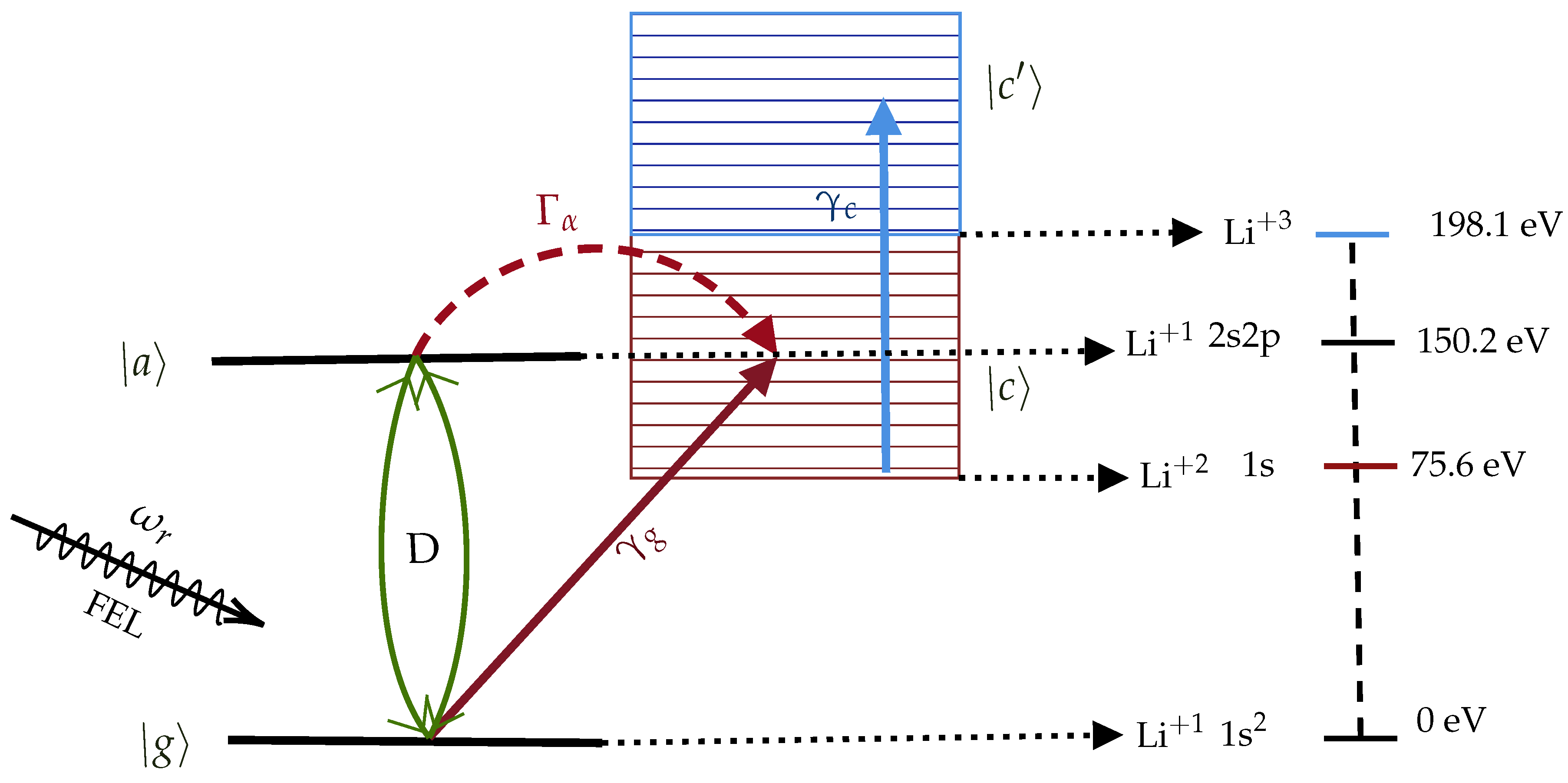
It is convenient to study the ionization process in the Fano-representation which consists to separate the two-electron eigenstates into its bound and continuum part. In Figure 1, the interaction scheme of Li${}^{+}$ with a FEL pulse is given. The artificial separation of the continuum two-electron wavefunction leads to an effective bound-bound and bound-continuum transition amplitudes which lead to ionization via two different pathways. The first channel initiates with a photon absorption from the ground state, $|g\rangle$, to the artificial Fano-bound state, $|a\rangle$ coupled with the Fano-continuum states, $|c\rangle$, via the interelectronic interaction, $V_{ac}$, operator; the latter rate of decay is given by the AIS width, ${\Gamma }_a$ while the rate of excitation is determined by the dipole transition matrix element, $d_{ga}$. At the same time, photoionization via a direct transition ($d_{gc}$) from the ground state to the Fano continuum, $|c\rangle$, is also available. The interference between the two ionization channels ($|g\rangle \to \left(d_{ga}\right)\to |a\rangle \to \left(V_{ac}\right)\to |c\rangle$ and $|g\rangle \to \left(d_{gc}\right)\to |c\rangle$ leads to the well known Fano-asymmetric shape [23].

More specifically, the ground-state $|g\rangle$ (1s${}^2$) is considered to be at $E_g=0$ eV (0 a.u.) and the FEL pulse’s central frequency $\omega$ is chosen near the resonance energy of $|a\rangle$ (2s2p). The system ionizes into the continuum $|c\rangle$ (ionization potential at 75.6 eV (2.778 a.u.)) characterised by the field-dependent photoionization width ${\gamma }_g\left(t\right)$; also the system, following photon absorption by the field, may excite to the unstable doubly excited auto-ionizing state $|a\rangle$ ($E_a=150.2$ eV (5.52 a.u.)) with a rate characterized by the field dependent Rabi matrix element $D\epsilon \left(t\right)$ coupled with continuum $|c\rangle$. The interference between these two ionizing channels is described by the introduction of the Fano-parameter $q_a$. Finally, the generated Li${}^{2+}$ may further ionize by absorbing one more photon since its ionization potential is 198–75.6 eV (triple ionization of Li ~ 198.1 eV (7.28 a.u.)). We characterize this ionization width as ${\gamma }_c$.

From the above, we see that there arises the need to calculate, $E_a,{\Gamma }_a,d_{ga},d_{gc}$ and $q_a$. Below we give the absolutely necessary formulas for these calculations. The procedure is as follows: (a) from the numerically calculated two-electron states we calculate the photoionization cross section and the position and width of the autoionizing resonance and (b) from these values we calculate the Fano effective parameters, $d_{ga},d_{gc},q_a$.

2.2.1. Photoionization Cross Section and Position, width of the Autoionizing Resonance

The photoionization cross sections of Li${}^{+}$ in a.u. is calculated by,

$${\sigma }_1\left(E_n\right)=\frac{4{\pi }^2}{c}\omega |\langle {\Phi }_{E_{1}S}|z_1+z_2|{\Phi }_{E_{n}P}{\rangle |}^2=\frac{4{\pi }^2}{c}\omega {\left|d_{1S;nP}\right|}^2,E_n=E_1+\omega ,$$

(6)

where $\omega$ is the central carrier frequency of the laser field, ${\Phi }_{E_{1}S}$, ${\Phi }_{E_{n}P}$ represent the initial (ground state) and the final (near AIS) states of the system and $z_1,z_2$ the electron’s position operators. A plot of this cross section is given in Reference [20].

Standard theory of the atomic continuum states shows that if the total singly-ionized wave function (above the first ionization threshold) is decomposed as the sum of a bound doubly excited state, its continuum background and all the other zero-order states included, a simple relation for the continuum state’s phase shift near the autoionizing states and its position and the width exists:

$${\delta }_l\left(E\right)=b_0+b_{1}E+b_2{E}^2+{\tan }^{-1}\frac{{\Gamma }_a/2}{E_a-E},$$

(7)

where $E_a$ is the position of the autoionizing state, and ${\Gamma }_a$ is the autoionizing width of this state; $b_i{E}^i$ s represent the residual background energy dependence of the phase shift.

With the phase shift, ${\delta }_l\left(E\right)$ calculated numerically, a fit with the above relation provides the values of $E_a$ and ${\Gamma }_a$, shown in

Table 1. Atomic parameters in a.u. used for the Li${}^{+}\left(2s2p\right)$ AIS resonance.

Parameters	Widths
$(E_a,q_a)$	(5.52, −2.2)
$d_{ga}$	0.01527
${\Gamma }_a$	0.00235
${\gamma }_g$	0.0819
${\gamma }_c$	0.0584

.

The photoionization cross sections of the hydrogenic ion, Li${}^{++}$, is an easier task and calculated by,

$${\sigma }_1\left({ϵ}_{np}\right)=\frac{4{\pi }^2}{c}\omega |\langle {\varphi }_{1s}\left|z\right|{\varphi }_{np}{\rangle |}^2=\frac{4{\pi }^2}{c}\omega {\left|d_{1s;np}\right|}^2,{ϵ}_{np}={ϵ}_{1s}+\omega ,$$

(8)

where ${\varphi }_{1s}\left(\mathit{r}\right)$ and ${\varphi }_{np}\left(\mathit{r}\right)$ are the common eigenstates of the Li${}^{++}$ Hamiltonian, angular momentum and its $z–$axis projection. The energies, ${ϵ}_{1s},{ϵ}_{np}$ are obtained from the solution of the radial eigenvalue Equation (4). The matrix elements $d_{1s;np}$ have been calculated earlier [19,20].

At this point, for later use, the photoionization yield, caused by a monochromatic field of amplitude $E_0$ and frequency, $\omega$, should be related with the photoionization cross section. First we need to relate the intensity of a monochromatic electric field with its amplitude. This relation is obtained by taking the time-average of the Poynting vector magnitude, S, $I_0={\langle S\rangle }_t=c{ϵ}_0{E}_0^2/2$ and set ${\epsilon }_0=1/4\pi$, with ${\epsilon }_0$ the vacuum’s dielectric constant. This will give $I_0=c{E}_0^2/8\pi$. Then by use of standard perturbation theory the ionization yield is related with the photoionization cross section (all quantities in a.u.):

$${\overline{\gamma }}_{if}={\sigma }_1\frac{I_0}{\omega }=\frac{4{\pi }^2}{c}\omega |d_{if}{|}^2\frac{c{E}_0^2/8\pi }{\omega }=2\pi {\left|d_{if}\right|}^2\frac{E_0^2}{4}={\gamma }_{if}\mathcal{I},$$

(9)

where the bar emphasizes that we refer to a time-averaged ionization rate and is $\mathcal{I}$ defined as the time-averaged intensity $\mathcal{I}=E_0^2/4$. Now ${\gamma }_{if}$ represents the average ionization rate when $\mathcal{I}=1$. The above expression provides the ionization width when the cross section is known, and vice-versa. All the following formulas are expressed in terms of ionization width rather than the photoionization cross section.

2.2.2. Calculation of the Fano Parameters, $q_a,d_{ga},d_{gc}$

Having numerically calculated the total photoionization cross section, ${\sigma }_1\left(E\right),E=E_g+\omega$, the position and the width of the autoionizing state, $(E_a,{\Gamma }_a)$, we are able to use the Fano approach of the resonant autoionization where the transitions are separated to purely bound-bound and to bound-continuum transitions, as shown in Figure 1. The Fano transition matrix elements to be determined are the $q_a$,$d_{gc}$ and $d_{ga}$ Fano parameters.

In its simplest form, the Fano parametrization of the dipole photoionization cross section ionization expressed at energy $E=E_g+\omega =E_c=E_{nP}$ is written as,

$$\begin{array}{c}\hfill |d_{1S;nP}{|}^2=|d_{gc}{|}^2\frac{{(q+ϵ)}^2}{1+{ϵ}^2}={\left|d_{gc}\right|}^2(1+\frac{q_a^2-1+2q_aϵ}{1+{ϵ}^2}),ϵ=\frac{E-E_a}{\frac{1}{2}{\Gamma }_a}\end{array}$$

(10)

where $d_{1S;nP}$ is the dipole transition moment in Equation (8). $d_{gc}$ is the dipole transition moment from the ground state to the $|c\rangle$ state and $ϵ$ is the normalized photon energy. In the above parametrization formula, $q_a$ is dimensionless and describes the degree of asymmetry of the resonant line shape,

$$q_a=\frac{d_{ga}}{\pi d_{gc}{V}_{ca}},$$

(11)

where $V_{ca}$ represents the static interelectronic interaction operator $1/r_{12}$. Examination of Equation (10) shows that the ionization profile takes its extrema at the following positions,

$$E_c^{\left(max\right)}=E_a+\frac{{\Gamma }_a}{2q_a},E_c^{\left(min\right)}=E_a-\frac{1}{2}{\Gamma }_a{q}_a.$$

(12)

One can select either the minimum or the maximum of the profile to calculate the $q_a$ (given that $E_a,{\Gamma }_a$ are known). In fact, knowledge of ${\Gamma }_a$ is sufficient since, the $E_a$ can be eliminated by subtracting the above expressions to arrive at,

$$E_c^{\left(max\right)}-E_c^{\left(min\right)}=\frac{{\Gamma }_a}{2}(\frac{1}{q_a}+q_a)\to q_a=\frac{E_c^{\left(max\right)}-E_c^{\left(min\right)}}{{\Gamma }_a}\pm \sqrt{{\left(\frac{E_c^{\left(max\right)}-E_c^{\left(min\right)}}{{\Gamma }_a}\right)}^2-1}.$$

(13)

Obviously this formula eliminates any inaccuracy introduced in the calculation by the resonant position.

Following with the calculation of $d_{ga}$ we see from Equation (10) that there is an energy $\overline{E}$ where,

$$q_a^2+2q_a\overline{ϵ}-1=0\to \overline{E}=E_a+\frac{{\Gamma }_a}{2}\frac{1-q_a^2}{2q_a}\to |d_{gc}{|}^2{|}_{E=\overline{E}}={|d_{1S;nP}|}^2{|}_{E=\overline{E}}.$$

(14)

So we can calculate $d_{gc}$ from the above relation and by substituting its value in Equation (11) we obtain $d_{ga}$, given that ${\Gamma }_a=2\pi {\left|V_{\overline{E}}\right|}^2$. This determines the value of $d_{ga}$ up to a sign value, but this can be infered from the ionization profile shape, which also determines the relative sign of $d_{ga}$ and $d_{gc}{V}_{cg}$. This means that the sign for $d_{gc}$ and $V_{cg}$ (which results to a definite sign for $d_{gc}{V}_{cg}$) will not affect the dynamics of the ionization; the $d_{ga}$ will obtain a value dependent on this choice and the sign of $q_a$.

Finally, for later use another useful relation between the Fano parameters is valid:

$$4|d_{ga}{|}^2=q_a^2{\Gamma }_a{\gamma }_g.$$

(15)

Following the above methodology for the calculation of the Fano parameters of the $2s2p{}^{1}P$ state of Li${}^{+}$ the obtained values are shown in Table 1.

Having calculated the necessary dynamic parameters for the description of the ionization processes we are now at a position to set up the equation-of-motions (EOMs) for the system’s probability amplitudes. In the present work we’ll be using a density-matrix representation to describe the quantum states of the systems and a semiclassical representation of the (stochastic) FEL field.

3. The Density-Matrix EOMs in the Fano Representation

The pulses of FEL radiation differ from shot to shot due to the inherent randomness [13]. This affects the process of obtaining the atomic observables. For a certain class of experiments the observables are the results of multishot interaction with the FEL radiation with the result that any calculation requires the average over an ensemble of shots. Our starting point is to derive the density matrix equation for a FEL field, pretending that it is not fluctuating; this part of derivation is independent on the statistical properties of the field. Having derived these equation we’ll be assuming the case of random fluctuations of the FEL field and will proceed with the ensemble averaged form of the density-matrix equations. Both of these steps have been developed and described in detail previously and need not be elaborated with great detail here [12,21]. Nevertheless, some adaptations are still required and as such we will provide here the absolutely necessary information about the calculational methodology for the dynamics.

Our starting point for the first part will be the Liouville equation, $ı\widehat{\rho }\left(t\right)=[\widehat{H},\widehat{\rho }]$[24]. Here, $\widehat{\rho }\left(t\right)$ is the density matrix operator and $\widehat{H}$ is the Hamiltonian operator which is comprised of the field free Hamiltonian (${\widehat{H}}_a$) as well as the field-matter interaction operator ($\widehat{V}\left(\left(t\right)\right)$), that is, $\widehat{H}={\widehat{H}}_a+\widehat{D}\left(t\right)$. The field-matter interaction operator is given by $\widehat{D}\left(t\right)=-\widehat{d}E\left(t\right)$ where characterises the atomic dipole operator and the interacting linearly polarised laser field is modelled as $E\left(t\right)=E_o\left(t\right)$cos($\omega t+\varphi \left(t\right)$). This real field relates to the complex field envelope by the relation $\epsilon \left(t\right)=\frac{1}{2}{E}_0\left(t\right)e^{-ı\varphi \left(t\right)}$. With the complex field modelled as above, we may define the time averaged intensity as $\mathcal{I}\left(t\right)={\left|\epsilon \left(t\right)\right|}^2$.

When the interacting field is considered to be having a near resonant frequency, the field free evolution of the density matrices evolve with a time-scale proportional to $\omega \sim |E_a-E_g|$, whereas the presence of the field induces far lower timescales such as $|D_{ag}|<<\omega$. This fact can be exploited in eliminating the fast oscillating terms from the system. To this end, we may transform the density matrices into the interaction picture (IP) [21], where the diagonal elements are left intact and the off-diagonal elements are changed by a phase factor. The newly defined density matrix elements are related to the old by ${\sigma }_{ij}\left(t\right)={\rho }_{ij}\left(t\right)e^{ı(E_a-E_g)t}$.

It is assumed beforehand that the field-free eigen value problem is solved for the system of Li${}^{+}$. This gives the eigen state basis on which the density operator is expanded. It is also assumed that the dipole transition matrix elements between the eigen states of the system at play are already known. The final set of modified density matrix equations of motion (EOMs) are given below, in terms of analytic envelopes of the complex field $\epsilon \left(t\right)$ and time averaged intensity $\mathcal{I}\left(t\right)$.

$$\begin{array}{ll}{\dot{\sigma }}_{gg}\left(t\right)& =-{\gamma }_g\mathcal{I}\left(t\right){\sigma }_{gg}\left(t\right)+2\mathrm{I}\mathrm{m}\left[\mathcal{D}\epsilon \left(t\right){\sigma }_{ag}\left(t\right)\right],\end{array}$$

(16a)

$$\begin{array}{ll}{\dot{\sigma }}_{aa}\left(t\right)& =-{\Gamma }_a{\sigma }_{aa}\left(t\right)-2\mathrm{I}\mathrm{m}\left[{\mathcal{D}}^{\ast }\epsilon \left(t\right){\sigma }_{ag}\left(t\right)\right]\end{array}$$

(16b)

$$\begin{array}{ll}{\dot{\sigma }}_{ag}\left(t\right)& =-\left[\delta +\Delta \mathcal{I}\left(t\right)\right]{\sigma }_{ag}\left(t\right)+ı{\mathcal{D}}^{\ast }{\epsilon }^{\ast }\left(t\right){\sigma }_{aa}\left(t\right)-ı\mathcal{D}{\epsilon }^{\ast }\left(t\right){\sigma }_{gg}\left(t\right)\end{array}$$

(16c)

$$\begin{array}{ll}{\dot{\sigma }}_{cc}\left(t\right)& =-{\gamma }_c\mathcal{I}\left(t\right){\rho }_{cc}\left(t\right)-{\dot{\sigma }}_{gg}\left(t\right)-{\dot{\sigma }}_{aa}\left(t\right).\end{array}$$

(16d)

$Im\left(z\right)\equiv (z-z^{\ast })/2ı$. ${\gamma }_g=2\pi {\left|d_{gc}\right|}^2$ and ${\gamma }_c=2\pi {\left|d_{1s;ϵp}\right|}^2$ are the ionization widths at peak intensity from the ${\Phi }_g$ initial state to the Fano continuum state $|c\rangle$ and from ${\varphi }_{1s}$ (Li${}^{2+}$ ground state) to the continuum state ${\varphi }_{np}$ (Li${}^{2+}$ continuum state), respectively. ${\Gamma }_a=2\pi {\left|V_{ac}\right|}^2$ is the autoionization width from the Fano state $|a\rangle$ to the Fano continuum states $|c\rangle$. $\Delta ,\delta$ are the complex peak detunings,

$$\delta =ı(E_a-E_g-\omega )+\frac{{\Gamma }_a}{2},\Delta =ı(s_a-s_g)+\frac{{\gamma }_g}{2},$$

(17)

with $s_g,s_a$ the peak intensity ac-Stark shifts (which are negligible for the intensities considered in this work). Finally, $\mathcal{D}$ is the complex Rabi transition matrix element,

$$\mathcal{D}=d_{ga}(1-\frac{i}{q_a}),$$

(18)

where $d_{ga}$ represents now the real part of the transition matrix element between the ground $|g\rangle$ and the excited $|a\rangle$ state. The interference between the two ionization channels is represented from the imaginary part of $\mathcal{D}$. For $q_a\gg 1$ the indirect ionization channel dominates whereas in the opposite case ionization proceeds via the direct path ($|g\rangle \to |c\rangle$).

4. The Averaged Density-Matrix EOMs

In the below we first specify the statistical model chosen for the FEL in this work. Based on this model, we provide the corresponding ensemble-averaged EOMs equations for Equations (16). Since the detailed derivation of the averaged EOMs for the density-matrix elements in the Fano representation is presented in Reference [12] here we only provide the final form as they are specified for the chosen model of the FEL field.

4.1. FEL Radiation as a Gaussian, Non-Stationary Stochastic Process

The temporal fluctuations of the field are taken into account by treating the pulse envelope as a stochastic process, more specifically,

$$\epsilon \left(t\right)={\epsilon }_0\left(t\right)ϵ\left(t\right)$$

(19)

The $ϵ\left(t\right)$ random process is used to describe the statistical properties of the field whereas the ${\epsilon }_0\left(t\right)$ represents the real slowly varying field envelope. The statistics of the fluctuations are assumed to be fully characterised by the multitime moments (coherences) $\langle ϵ\left(t_1\right)ϵ\left(t_2\right)\cdots ϵ\left(t_n\right)\rangle$. The approach taken here is to assume that the field is a Gaussian stochastic process, which in practice means that its full description requires only the knowledge of its first and second coherence; this is because all the multitime moments are expressed in terms of the first two moments.

More specifically, we assume the model adopted by Krinsky and Li in Reference [13] for FEL radiation where, deterministic part of the field envelope is taken as,

$${\epsilon }_0\left(t\right)={\epsilon }_0{e}^{-\widehat{\chi }{t}^2/2{\tau }_p^2},$$

(20)

where ${\tau }_p$ determines the FWHM duration of the pulse and chirp $\widehat{\chi }=1-ı/\sqrt{3}$. The first- and the second- moment of the field are assumed,

$$\langle ϵ\left(t\right)\rangle =0,\langle ϵ\left(t\right){ϵ}^{\ast }(t-\tau )\rangle =e^{-{\tau }^2/2{\tau }_c^2},$$

(21)

where ${\tau }_c$ is the coherence time. With the above assumptions we have for the statistically averaged intensity and the first-order intensity coherence function,

$$\langle \mathcal{I}\left(t\right)\rangle ={\langle \left|\epsilon \left(t\right)\right|}^2\rangle ={\epsilon }_0^2{e}^{-t^2/{\tau }_p^2},\langle \mathcal{I}\left(t\right)\mathcal{I}\left(t^{\prime }\right)\rangle =\langle \mathcal{I}\left(t\right)\rangle \mathcal{I}\langle \left(t^{\prime }\right)\rangle +{\left|\langle \epsilon \left(t\right)\epsilon \left(t^{\prime }\right)\rangle \right|}^2.$$

(22)

The full width half maximum ${\tau }_{FWHM}$ of the average intensity $\langle \mathcal{I}\left(t\right)\rangle$ is related to the pulse duration ${\tau }_p$ via ${\tau }_{FWHM}=2{\tau }_p\sqrt{ln2}$. Therefore the FEL is represented as a Gaussian, non-stationary, square-exponentially correlated stochastic process.

4.2. Averaged Form of the EOMs

The presence of the FEL temporal fluctuations render the field to be treated statistically, as a stochastic process, thus making the EOMs for the system to be stochastic differential equations. Let’s assume an arbitrary observable as $X\left(t\right)$ and consider it as a stochastic process. We can always decompose this into a deterministic and a fluctuating part that is, $X\left(t\right)=\langle X\left(t\right)\rangle +\tilde{X}\left(t\right)$, where $\langle X\left(t\right)\rangle$ is the ensemble average over many shots of the random FEL field and the $\tilde{X}\left(t\right)$ is a fluctuating quantity with zero mean average, $\langle \tilde{X}\left(t\right)\rangle =0$. For the electric field we have $\langle \epsilon \left(t\right)\rangle =0$ and $\epsilon \left(t\right)=\tilde{\epsilon }\left(t\right)$. When $X\left(t\right)$ represents the intensity, we have $\mathcal{I}\left(t\right)=\langle \mathcal{I}\left(t\right)\rangle +\tilde{\mathcal{I}}\left(t\right)$. In the deterministic EOMs Equation (16) the atomic structure parameters are coupled with the field’s random variations. Since generally $\langle {\sigma }_{ij}\left(t\right)\epsilon \left(t\right)\rangle \ne \langle {\sigma }_{ij}\left(t\right)\rangle \langle \epsilon \left(t\right)\rangle$ and $\langle {\sigma }_{ij}\left(t\right)\mathcal{I}\left(t\right)\rangle \ne \langle {\sigma }_{ij}\left(t\right)\rangle \langle \mathcal{I}\left(t\right)\rangle$ where $i,j=g,a,c$, special statistical methods need to be carefully employed. We have followed a method to obtain the statistical average of the EOMs given the FEL statistical properties; we’ll not elaborate the method further here as it has been worked in detail in Reference [12]. We only present the averaged EOMs for the system’s density matrix as adapted in the particular Gaussian, non-stationary FEL chosen with statistics as expressed in Equations (19)–(21).

We finally arrive at the following set of averaged density matrix EOMs in the Fano representation:

$$\begin{array}{ll}\langle {\dot{\sigma }}_{gg}\left(t\right)\rangle & =-{\gamma }_g\langle \mathcal{I}\left(t\right)\rangle \left[1-{\gamma }_g{\tau }_c\sqrt{\pi }\frac{\langle I\left(t\right)\rangle }{2}+\frac{{\Gamma }_a{\tau }_c\sqrt{\pi }}{2\sqrt{2}}\left[(q_a^2-1)U(\frac{{\widehat{\delta }}_{-}{\tau }_c}{\sqrt{2}})+2q_{a}V(\frac{{\widehat{\delta }}_{-}{\tau }_c}{\sqrt{2}})\right]\right]\langle {\sigma }_{gg}\left(t\right)\rangle \\ & +(q_a^2+1)\frac{{\Gamma }_a{\gamma }_g{\tau }_c\sqrt{\pi }\langle I\left(t\right)\rangle }{2\sqrt{2}}U(\frac{{\widehat{\delta }}_{+}{\tau }_c}{\sqrt{2}})\langle {\sigma }_{aa}\left(t\right)\rangle \end{array}$$

(23a)

$$\begin{array}{ll}\langle {\dot{\sigma }}_{aa}\left(t\right)\rangle & =-{\Gamma }_a\left[1+\frac{{\gamma }_g{\tau }_c\sqrt{\pi }\langle \mathcal{I}\left(t\right)\rangle }{2\sqrt{2}}\left[(q_a^2-1)U(\frac{{\widehat{\delta }}_{+}{\tau }_c}{\sqrt{2}})-2q_{a}V(\frac{{\widehat{\delta }}_{+}{\tau }_c}{\sqrt{2}})\right]\right]\langle {\sigma }_{aa}\left(t\right)\rangle \\ & +(q_a^2+1)\frac{{\Gamma }_a{\gamma }_g{\tau }_c\sqrt{\pi }\langle I\left(t\right)\rangle }{2\sqrt{2}}U(\frac{{\widehat{\delta }}_{-}{\tau }_c}{\sqrt{2}})\langle {\sigma }_{gg}\left(t\right)\rangle \end{array}$$

(23b)

$$\begin{array}{ll}\langle {\dot{\sigma }}_{cc}\left(t\right)\rangle & =-{\gamma }_c\langle \mathcal{I}\left(t\right)\rangle \langle {\sigma }_{cc}\left(t\right)\rangle -\langle {\dot{\sigma }}_{gg}\left(t\right)\rangle -\langle {\dot{\sigma }}_{aa}\left(t\right)\rangle +{\gamma }_c{\tau }_c\sqrt{\pi }\frac{{\langle I\left(t\right)\rangle }^2}{2}\left({\gamma }_c\langle {\sigma }_{cc}\left(t\right)\rangle -{\gamma }_g\langle {\sigma }_{gg}\left(t\right)\rangle \right),\end{array}$$

(23c)

where the averaged dynamic detunings, ${\widehat{\delta }}_{\pm }\equiv {\widehat{\delta }}_{\pm }\left(t\right)$, are defined by,

$${\widehat{\delta }}_{\pm }\left(t\right)={\delta }_0\pm ı\frac{{\Gamma }_a-{\gamma }_g\langle \mathcal{I}\left(t\right)\rangle }{2}.$$

(24)

From our atomic-structure calculations we have estimated that the ac-Stark shifts of the bound states and the direct photoionization from the doubly excited state have negligible contribution into dynamics compared to the parameters finally kept in the averaged EOMs.

The $U\left(z\right)=U(x,y),V\left(z\right)=U(x,y)$ quantities, closely related with the Voight functions, are defined as the real and imaginary of $w\left(z\right)$ [25]:

$$w\left(z\right)=e^{-z^2}[1-\mathrm{erf}(ız)]=U(x,y)+ıV(x,y),z=x-ıy,$$

(25)

where erf$\left(z\right)$ is the error function.

5. Results and Discussion

In this section, we show the results obtained from the averaged EOMs for the Li${}^{+}$ system for the schematic depicted in the Figure 1. First, we discuss the typical AIS lineshape which is obtained when no fluctuations are included. Then we see how the fluctuation’s coherence time of the FEL pulse affects this AIS lineshape. The calculated atomic parameters $q_a$ and ${\Gamma }_a$ are in good agreement with those measured in References [26,27,28] and presented in the Table 1.

5.1. The AIS Line Shape

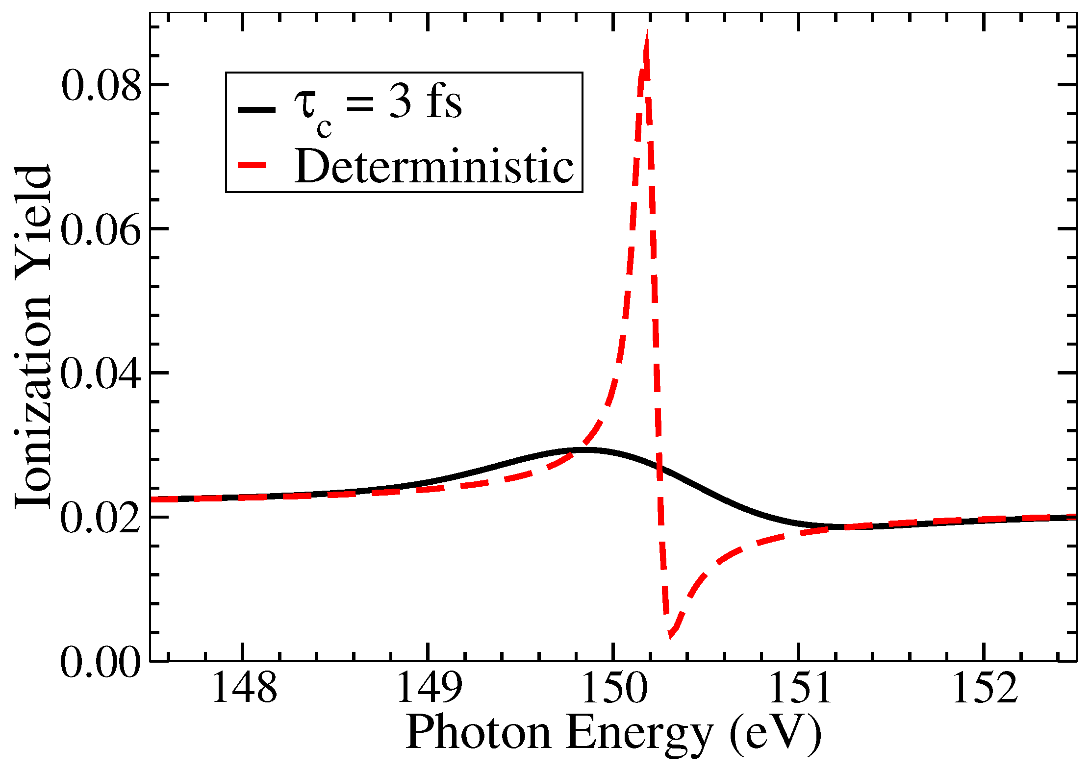
For a pulse of moderate intensity, free of fluctuations in the amplitude and the phase, the AIS lineshape of Li${}^{+}$ 2s2p should resemble that of the familiar asymmetric Fano profile [23]. Our findings show that the fluctuations cause a smoothing effect of such sharp asymmetric line shapes. Solving Equation (16) for a deterministic pulse, gives the ionization yield profile depicted by the red-dashed curve of the Figure 2, whereas solving Equation (23) for a Gaussian correlated stochastic pulse, having a coherence time of ${\tau }_c=1.3$ fs (53.74 a.u.), gives the ionization yield profile depicted by the black-solid curve of the Figure 2. The peak intensity used is 10${}^{13}$ W/cm${}^2$ and the pulse duration used is ${\tau }_p=12.7$ fs (525.02 a.u.).

It can be seen that for the same pulse duration and peak intensity we obtain drastically different yield values and lineshapes. The deterministic pulse, as pointed, gives the profile which has a sharp peak and asymmetry around the resonance energy whereas the stochastic pulse gives a smooth peak. The values of the ionization yield are also very different around the resonance but are identical towards the tail-ends. It can be thus concluded that the effects of fluctuations manifest and smooths the lineshape around the resonance, whereas the tail-ends are relatively unaffected.

5.2. Effects of the Fluctuation’s Coherence Time

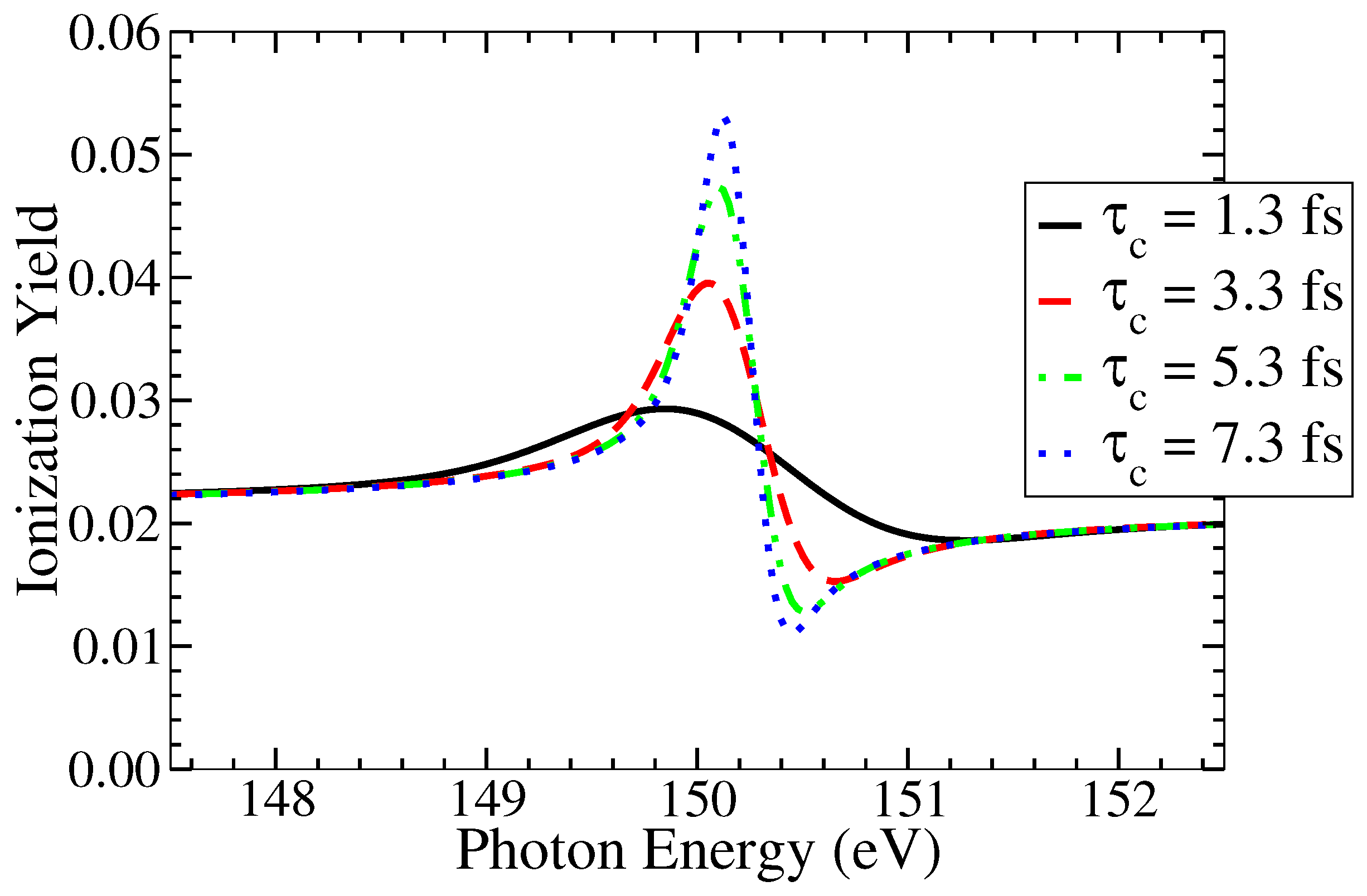
For the Gaussian pulse we use the coherence time which is decisive for the ionization dynamics. In Figure 3, we choose four values for the ${\tau }_c$, 1.3 fs, 3.3 fs, 5.3 fs and 7.3 fs (53.74 a.u., 136.42 a.u., 219.1 a.u. and 301.78 a.u., correspondingly). It can be seen from the said figure that as coherence time increases, the ionization yield around the resonance increases which is accompanied by a narrowing of the AIS lineshape. Ideally, for very large ${\tau }_c$, these lineshapes tend towards an asymmetric Fano-shape. This trend can be clearly seen here. It can also be observed that the effects of coherence time manifest only around the resonance. Towards the tail ends, the effects are negligible and the yield values are fairly constant.

5.3. Effects of the Pulse Duration

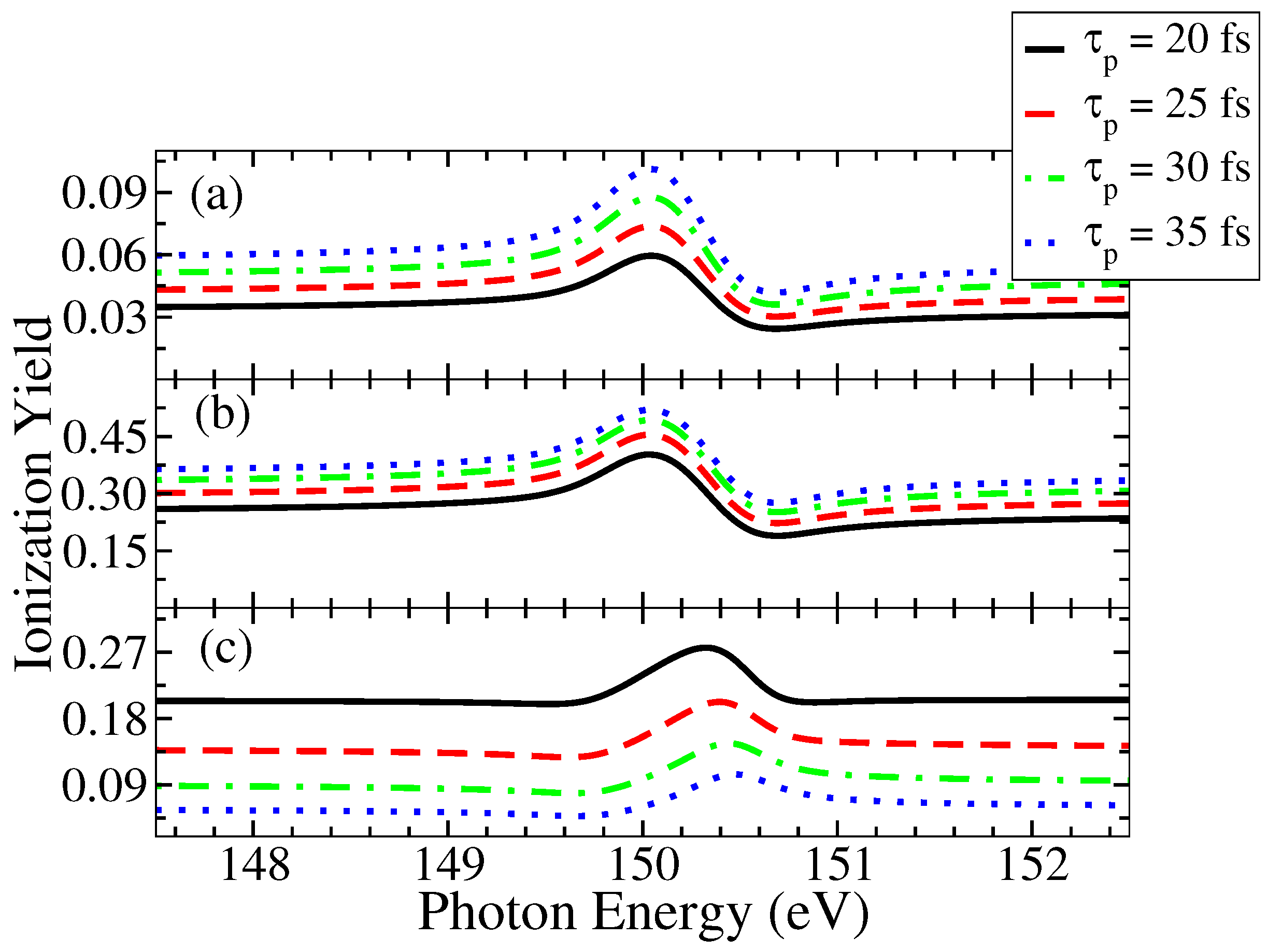
Since the pulse duration determines the interaction time with the system it is reasonable to expect that the longer the pulse the more is the ionization yield (this might not be the case under special resonance conditions). Here, we explore the role of pulse duration in affecting the ionization yield for different peak intensities.

In Figure 4, (a) is plotted for the peak intensity of 10${}^{13}$ W/cm${}^2$, (b) is for the peak intensity of 10${}^{14}$ W/cm${}^2$ and (c) is for the peak intensity of 10${}^{15}$ W/cm${}^2$. For (a) and (b) the trend of the yield is that, as pulse duration increases, the yield also increases. But for (c), the trend is reversed. As the peak intensity increases, the yield values decrease. This reversing of the behavior is due to the extra channel of ionization of Li${}^{2+}$ from $|c\rangle \to |c^{\prime }\rangle$ which is rapidly active at higher peak intensities that is, as peak intensity increases, the population of $|c\rangle$ decreases and the system ionizes into $|c^{\prime }\rangle$. The same is true with increasing pulse duration as well. That is why, at the highest peak intensity, the ionization yield values are low for the largest pulse duration and high for the smallest pulse duration.

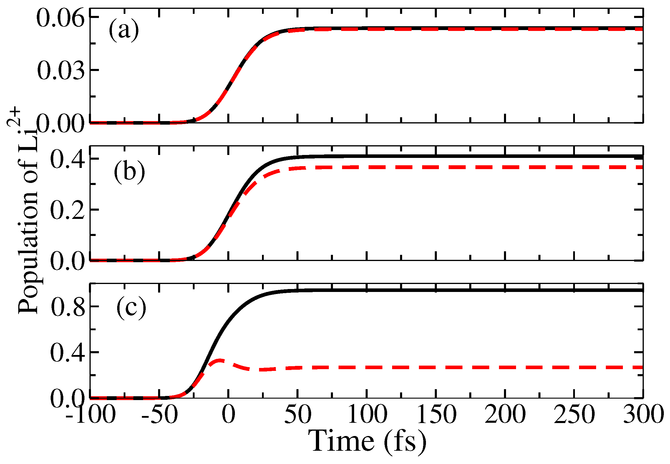
To understand this behavior, we may have to explore the time-evolution of the population of Li${}^{2+}$. In Figure 5, we plot the population of Li${}^{2+}$ in time for various peak intensities. The black-solid curve is for the situation when the further channel of ionization is not considered (${\gamma }_c=0$ a.u.) whereas the red-dashed curve is for the current situation where the said channel is present. In the former case, the expected behaviour, namely that by increasing the ${\tau }_p$ increases the ionization yield applies; the plots (a) and (b) depict the rise of populations even after the peak of the pulse (at t = 0 fs) has hit the system. In contrast, for the highest peak intensity, the population of Li${}^{2+}$ reaches a maximum before the peak of the pulse and the same population starts to decrease as pulse evolves. This clearly drops the ionization yield values which is the cause for the aforementioned trend-change in Figure 4.

6. Conclusions

We have investigated the effects of the FEL parameters such as peak-intensity, coherence time and pulse duration on the values of ionization yield of the Li${}^{+}$ resonance lineshapes. A safe conclusion is that the interaction with a FEL radiation results to lineshapes that may differ from the familiar Fano-like asymmetry shape. A better insight has been obtained about the role of the temporal fluctuations of the FEL field via their strength and duration.

We have considered the pulsed nature of the FEL by assuming a Gaussian envelope for the field and have taken the first-order coherence function to possess a square-exponential (Gaussian) time dependence, ∼$e^{-{(t_1-t_2)}^2/2{\tau }_c^2}$; this choice is different from those that have been assumed so far, when averaging of the EOMs was taken into account as for example ∼$e^{-|t_1-t_2|/2{\tau }_c}$ of the early lasers of longer-wavelength. The Gaussian-like dependence has been treated to date only within a Monte-Carlo (MC) algorithm type of calculations [9,10]. One of the outcomes is that the dynamics for relatively moderate intensity fields (∼$5\times {10}^{14}$ W/cm${}^2$) is determined by directly measured experimental observables, namely its temporal mean intensity and its power spectrum; more accurately, the autocorrelation (AC) functions of the time-integrated electric field amplitude and intensity, $\langle \epsilon \left(t\right){\epsilon }^{\ast }\left(t^{\prime }\right)\rangle$ and $\langle \mathcal{I}\left(t\right)\mathcal{I}\left(t^{\prime }\right)\rangle$, respectively. A second outcome is that the line profile takes the shape of a Voight profile with the Gaussian or the Lorentzian profile to dominate depending on the pulse parameters and the atomic structure.

References

- Wabnitz, H.; Bittner, L.; de Castro, A.R.B.; Dohrmann, R.; Gurtler, P.; Laarmann, T.; Laasch, W.; Schulz, J.; Swiderski, A.; von Haeften, K.; et al. Multiple ionization of atom clusters by intense soft X-rays from a free-electron laser. Nature 2002, 420, 482. [Google Scholar] [CrossRef]
- Ackermann, W.; Asova, G.; Ayvazyan, V.; Azima, A.; Baboi, N.; Bahr, J.; Balandin, V.; Beutner, B.; Brandt, A.; Bolzmann, A.; et al. Operation of a free-electron laser from the extreme ultraviolet to the water window. Nat. Photonics 2007, 1, 336. [Google Scholar] [CrossRef]
- Young, L.; Kanter, E.P.; Krässig, B.; Li, Y.; March, A.M.; Pratt, S.T.; Santra, R.; Southworth, S.H.; Rohringer, N.; DiMauro, L.F.; et al. Femtosecond electronic response of atoms to ultra-intense X-rays. Nature 2010, 466, 56–61. [Google Scholar] [CrossRef] [PubMed]
- Allaria, E.; Badano, L.; Bassanese, S.; Capotondi, F.; Castronovo, D.; Cinquegrana, P.; Danailov, M.; D’Auria, G.; Demidovich, A.; De Monte, R.; et al. The FERMI free-electron lasers. J. Synchrotron Radiat. 2015, 22, 485–491. [Google Scholar] [CrossRef] [PubMed]
- Tiedtke, K.; Azima, A.; von Bargen, N.; Bittner, L.; Bonfigt, S.; Düsterer, S.; Faatz, B.; Frühling, U.; Gensch, M.; Gerth, C.; et al. The soft X-ray free-electron laser FLASH at DESY: Beamlines, diagnostics and end-stations. New J. Phys. 2009, 11, 023029. [Google Scholar] [CrossRef]
- Nikolopoulos, L.A.A.; Kelly, T.J.; Costello, J. Theory of ac Stark splitting in core-resonant Auger decay in strong X-ray fields. Phys. Rev. A 2011, 84, 063419. [Google Scholar] [CrossRef] [Green Version]
- Nayak, A.; Dumergue, M.; Kühn, S.; Mondal, S.; Csizmadia, T.; Harshitha, N.; Füle, M.; Kahaly, M.U.; Farkas, B.; Major, B.; et al. Saddle point approaches in strong field physics and generation of attosecond pulses. Phys. Rep. 2019, 833, 1–52. [Google Scholar] [CrossRef]
- Papadogiannis, N.A.; Nikolopoulos, L.A.A.; Charalambidis, D.; Tsakiris, G.D.; Tzallas, P.; Witte, K. On the feasibility of performing non-linear autocorrelation with attosecond pulse trains. Appl. Phys. B 2003, 76, 721–727. [Google Scholar] [CrossRef]
- Rohringer, N.; Santra, R. Resonant Auger effect at high X-ray intensity. Phys. Rev. A 2008, 77, 053404. [Google Scholar] [CrossRef] [Green Version]
- Nikolopoulos, G.M.; Lambropoulos, P. Effects of free-electron-laser field fluctuations on the frequency response of driven atomic resonances. Phys. Rev. A 2012, 86, 033420. [Google Scholar] [CrossRef] [Green Version]
- Mouloudakis, G.; Lambropoulos, P. Effects of field fluctuations on driven autoionizing resonances. Eur. Phys. J. D 2018, 72, 226. [Google Scholar] [CrossRef] [Green Version]
- Katravulapally, T.; Nikolopoulos, L.A.A. Perturbative theory of ensemble-averaged atomic dynamics in fluctuating laser fields. arXiv 2020, arXiv:2006.02477. [Google Scholar]
- Krinsky, S.; Li, Y. Statistical analysis of the chaotic optical field from a self-amplified spontaneous-emission free-electron laser. Phys. Rev. E 2006, 73, 066501. [Google Scholar] [CrossRef]
- Rice, S.O. Mathematical analysis of random noise. Bell Syst. Tech. J. 1944, 23, 282–332. [Google Scholar] [CrossRef]
- Evgeny Saldin, E.V.; Schneidmiller, M.Y. The Physics of Free Electron Lasers; Springer: Berlin/Heidelberg, Germany, 2000. [Google Scholar]
- Kim, K.J.; Huang, Z.; Lindberg, R. Synchrotron Radiation and Free-Electron Lasers, 1st ed.; Cambridge University Press: Cambridge, UK, 2017. [Google Scholar]
- Nikolopoulos, L.A.A.; Nakajima, T.; Lambropoulos, P. Direct versus Sequential Double Ionization of Mg with Extreme-Ultraviolet Radiation. Phys. Rev. Lett. 2003, 90, 043003. [Google Scholar] [CrossRef] [Green Version]
- Nikolopoulos, L.A.A. A package for the ab-initio calculation of one- and two-photon cross sections of two-electron atoms, using a CI B-splines method. Comput. Phys. Commun. 2003, 150, 140–165. [Google Scholar] [CrossRef]
- Hanks, W.; Costello, J.; Nikolopoulos, L. Two- and Three-Photon Partial Photoionization Cross Sections of Li+, Ne8+ and Ar16+ under XUV Radiation. Appl. Sci. 2017, 7, 294. [Google Scholar] [CrossRef] [Green Version]
- Hanks, W. Multi-photon Cross Section of Helium-like Ions Under Soft XUV Fields. Master’s Thesis, School of Physical Sciences, Dublin City University, Dublin, Ireland, 2017. [Google Scholar]
- Nikolopoulos, L.A.A. Elements of Photoionization Quantum Dynamics Methods; Morgan & Claypool Publishers: San Rafael, CA, USA, 2019; pp. 2053–2571. [Google Scholar] [CrossRef]
- Bachau, H.; Cormier, E.; Decleva, P.; Hansen, J.E.; Martin, F. Applications of B-splines in Atomic and Molecular Physics. Rep. Prog. Phys. 2001, 64, 1815. [Google Scholar] [CrossRef]
- Fano, U. Effects of Configuration Interaction on Intensities and Phase Shifts. Phys. Rev. 1961, 124, 1866. [Google Scholar] [CrossRef]
- Blum, K. Density Matrix Theory and Its Applications; Plenum Press: New York, NY, USA, 1981. [Google Scholar]
- NIST Digital Library of Mathematical Functions; Release 1.0.27 of 2020-06-15. Available online: http://dlmf.nist.gov/ (accessed on 15 June 2020).
- Diehl, S.; Cubaynes, D.; Bizau, J.M.; Wuilleumier, F.J.; Kennedy, E.T.; Mosnier, J.P.; Morgan, T.J. New high-resolution measurements of doubly excited states of Li+. J. Phys. B At. Mol. Opt. Phys. 1999, 32, 4193–4207. [Google Scholar] [CrossRef]
- Mosnier, J.P.; Costello, J.; Kennedy, E.; Whitty, W. The photoabsorption spectrum of laser-generated Li+ in the 60–190 eV photon energy range. J. Phys. B At. Mol. Opt. Phys. 2000, 33, 5203–5214. [Google Scholar] [CrossRef]
- Scully, S.W.J.; Álvarez, I.; Cisneros, C.; Emmons, E.D.; Gharaibeh, M.F.; Leitner, D.; Lubell, M.S.; Müller, A.; Phaneuf, R.A.; Püttner, R.; et al. Doubly excited resonances in the photoionization spectrum of Li+: Experiment and theory. J. Phys. B At. Mol. Opt. Phys. 2006, 39, 3957–3968. [Google Scholar] [CrossRef]
Figure 1.
Ionization scheme of Li. is the ground state, 2s2p is the auto-ionizing state, is the continuum above the ionized state of Li 1s and the is the continuum above the ionized state Li. The energies depicted on the right are not to scale but only give an idea of the values of the levels.
Figure 2.
The effect of smoothing the familiar Fano-profile, caused by averaging the fluctuations can be clearly seen in this figure. The red-dashed curve with highest peak is obtained for a deterministic pulse whereas the black-solid curve is obtained for a stochastic pulse with coherence time of 1.3 fs (53.74 a.u.). The peak intensity is 10 W/cm and the pulse duration fs (525.02 a.u.).
Figure 3.
Effect of coherence time on the ionization yield is shown in this plot. As increases, the ionization yield also increases, near resonance. The peak intensity is 10 W/cm and the pulse duration fs (525.02 a.u.).
Figure 4.
Effect of pulse duration on the ionization yield is shown in this plot. The coherence time used is fs (124.02 a.u.) and the peak intensities are: 10 W/cm for (a), 10 W/cm for (b) and 10 W/cm for (c). For lower intensities, as pulse duration increases, the ionization yield also increases. But the pattern flips after certain peak intensity and for the highest peak intensity of 10 W/cm, the yield drops as pulse duration increases.
Figure 5.
Effect of peak intensity on the population of Li. The peak intensities used are: 10 W/cm for (a), 10 W/cm for (b) and 10 W/cm for (c). Black-solid curve is when the further ionization channel is ignored () and the red-dashed curve is when the further ionization channel is considered. The pulse duration 20 fs (826.8 a.u.) and the coherence time 3 fs (124.02 a.u.). The red-dashed curve suggests that for (a) and (b) the population grows after the peak intensity at t = 0 fs, but for (c) it drops. This causes the change in the trend of ionization of Figure 4.