Predicting Deep Learning Based Multi-Omics Parallel Integration Survival Subtypes in Lung Cancer Using Reverse Phase Protein Array Data

 , , , ,
Abstract
:1. Introduction
2. Materials and Methods
2.1. TCGA Dataset
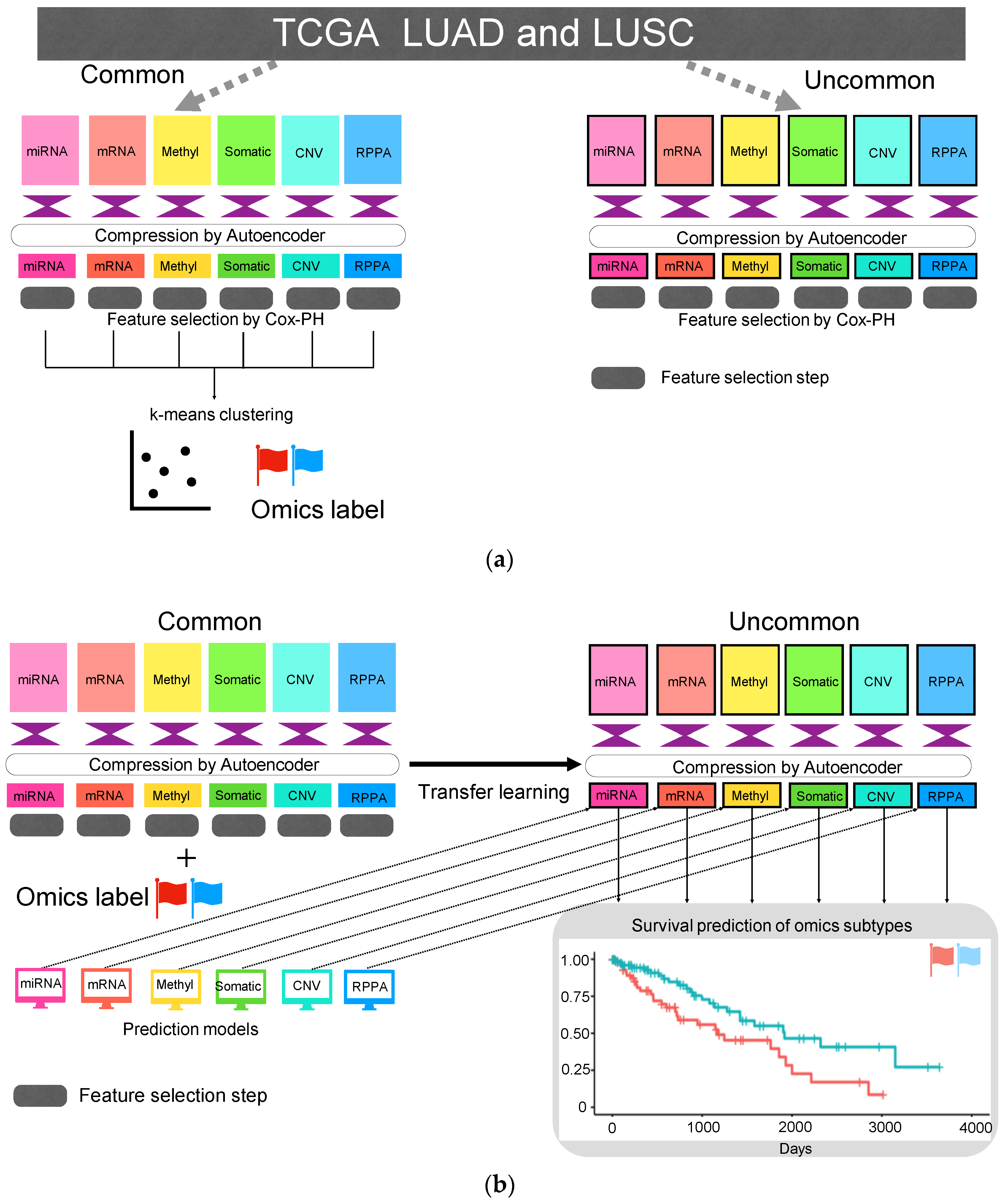
2.2. Autoencoder
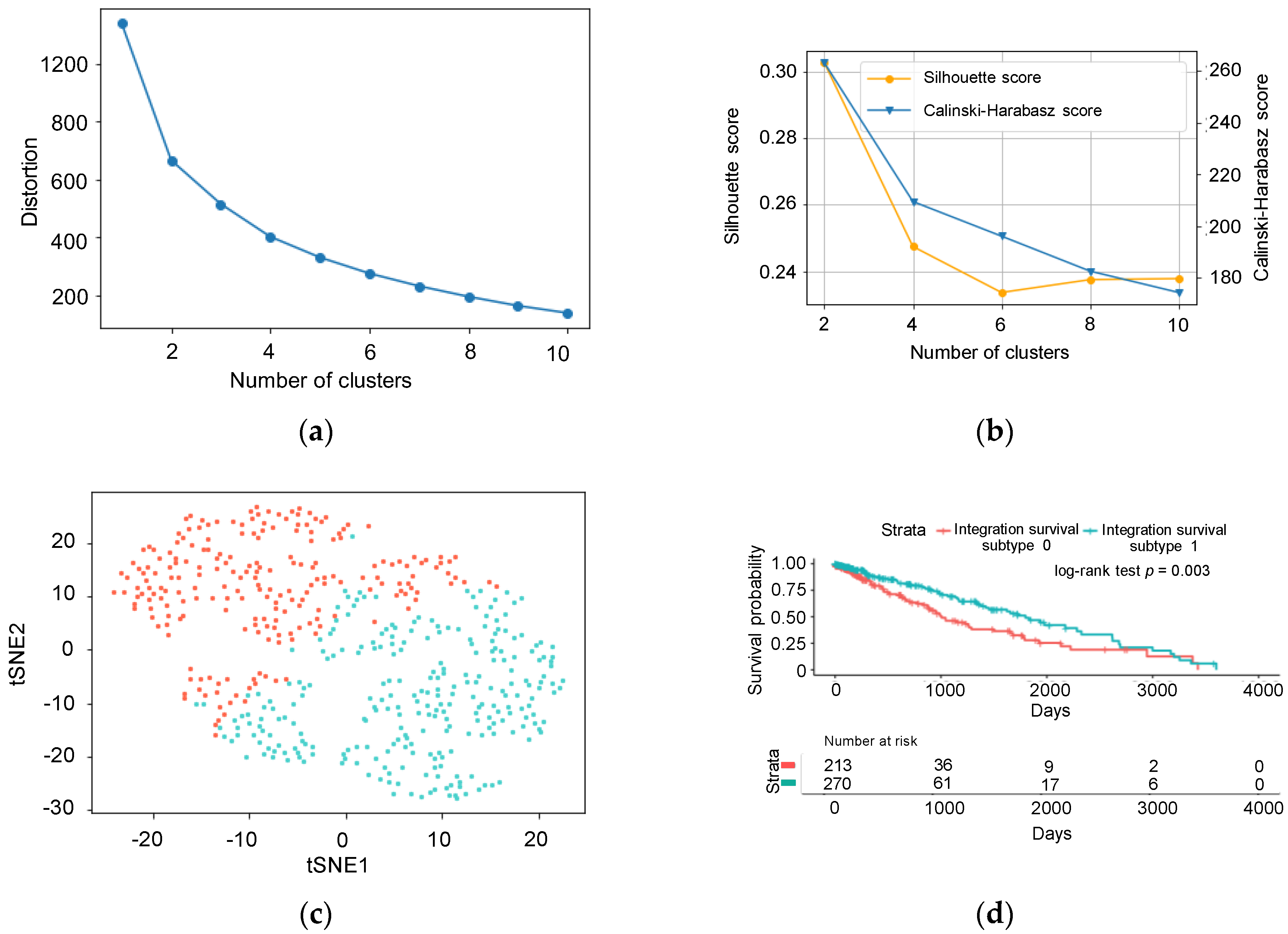
2.3. Feature Selection and k-Means Clustering
2.4. Machine Learning Models that Predict Cluster ID
2.5. Predict Cluster ID Using Compressed Uncommon Data
2.6. Identification of the Proteins Associated with Cluster ID
2.7. Statistical Analysis
3. Results
3.1. Unsupervised Approach for Obtaining Clinically Meaningful Subtypes
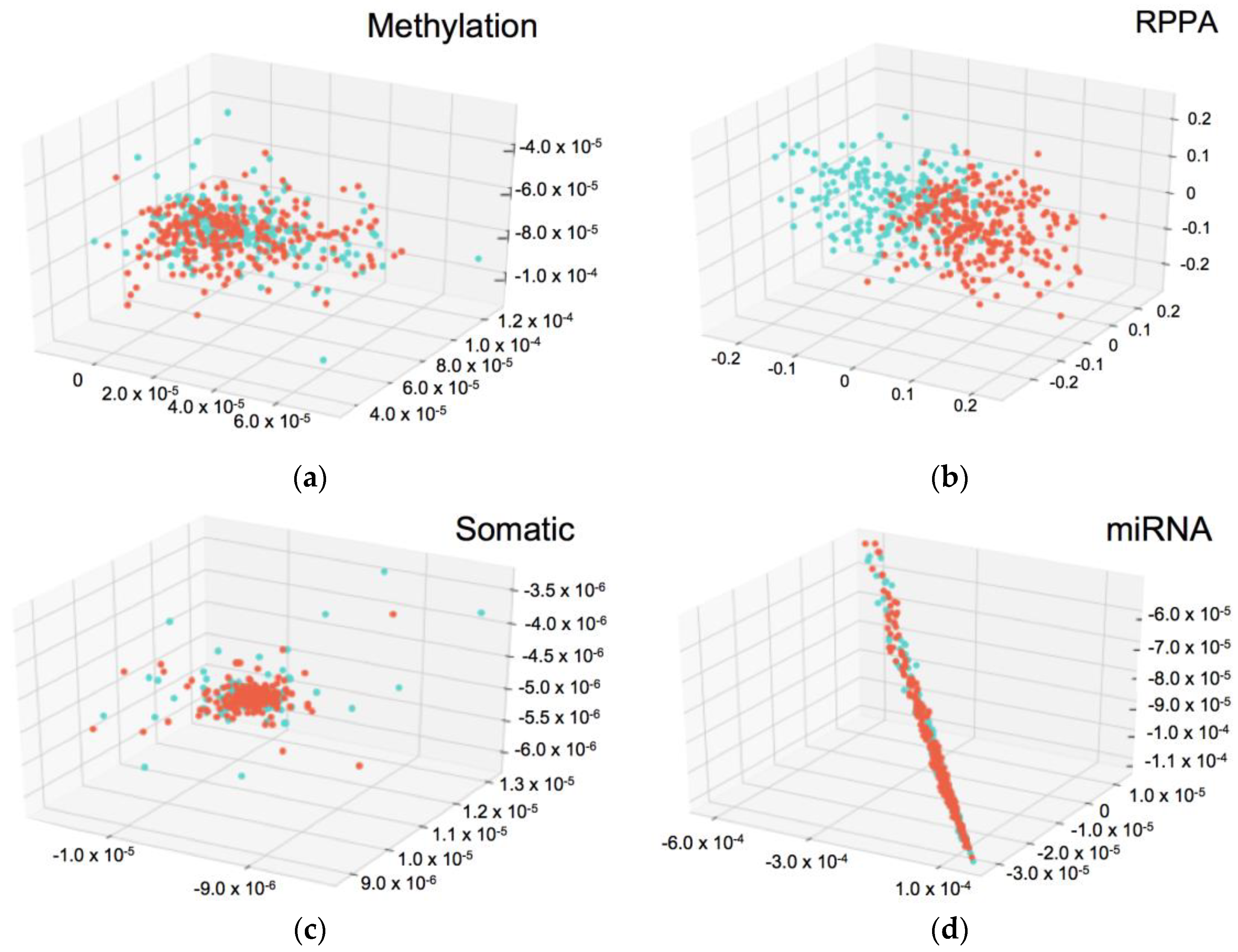
3.2. Predicting Integration Survival Subtypes Using Compressed Categorical Datasets
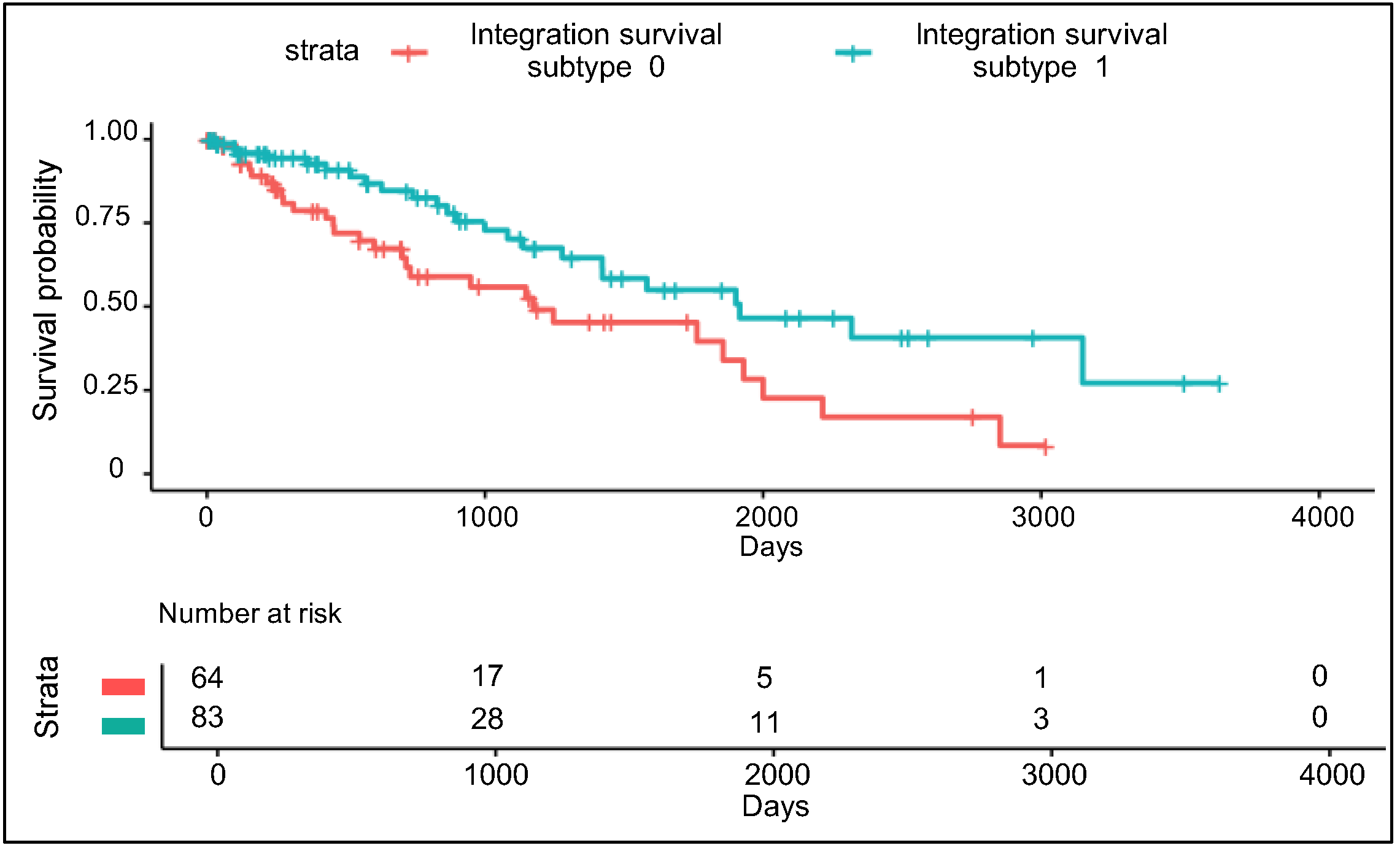
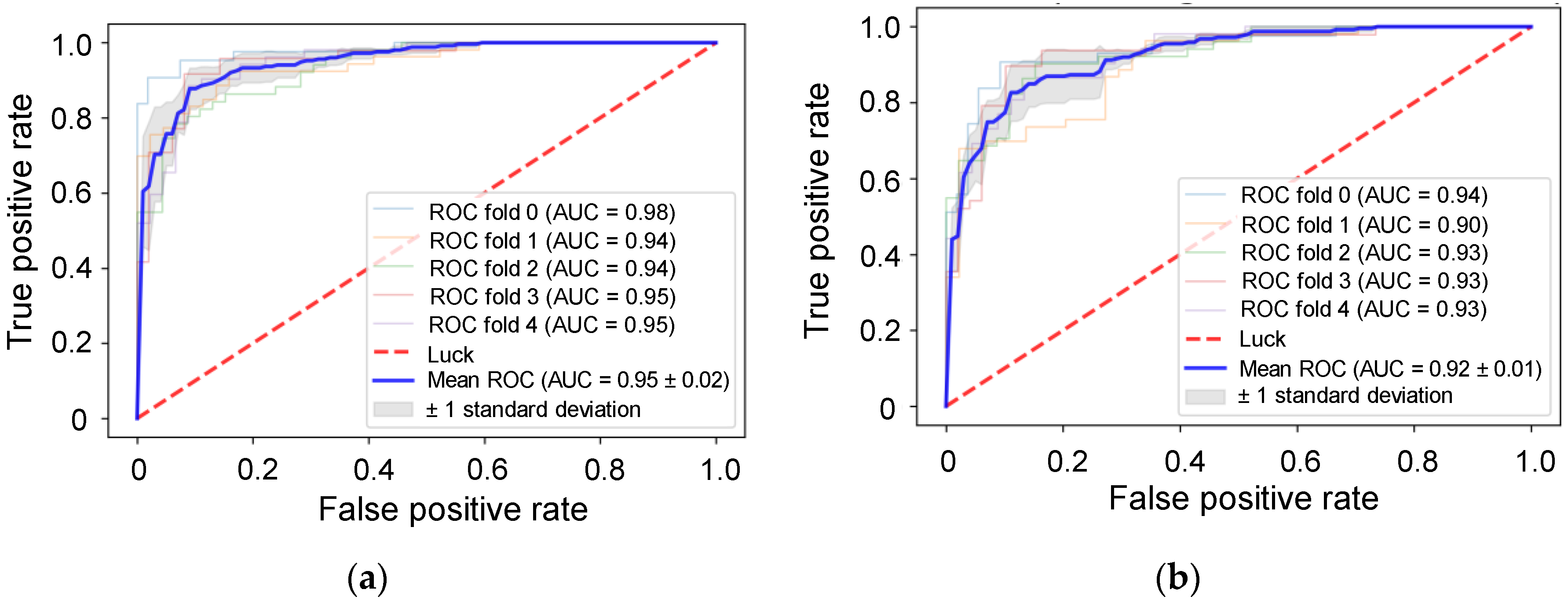
3.3. Validation Using Uncommon RPPA Datasets
3.4. Comparison of Integration Survival Subtypes and RPPA Survival Subtypes
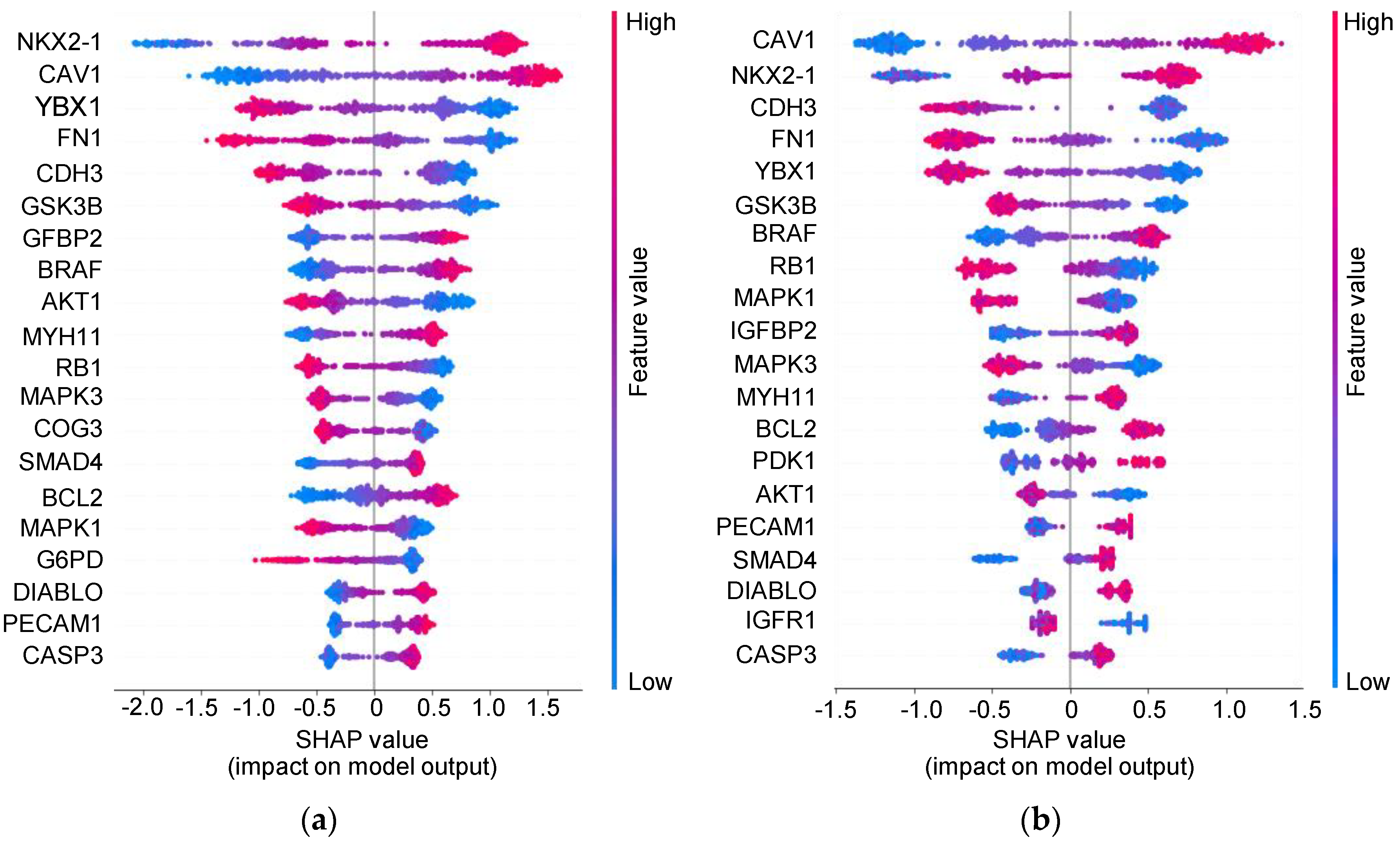
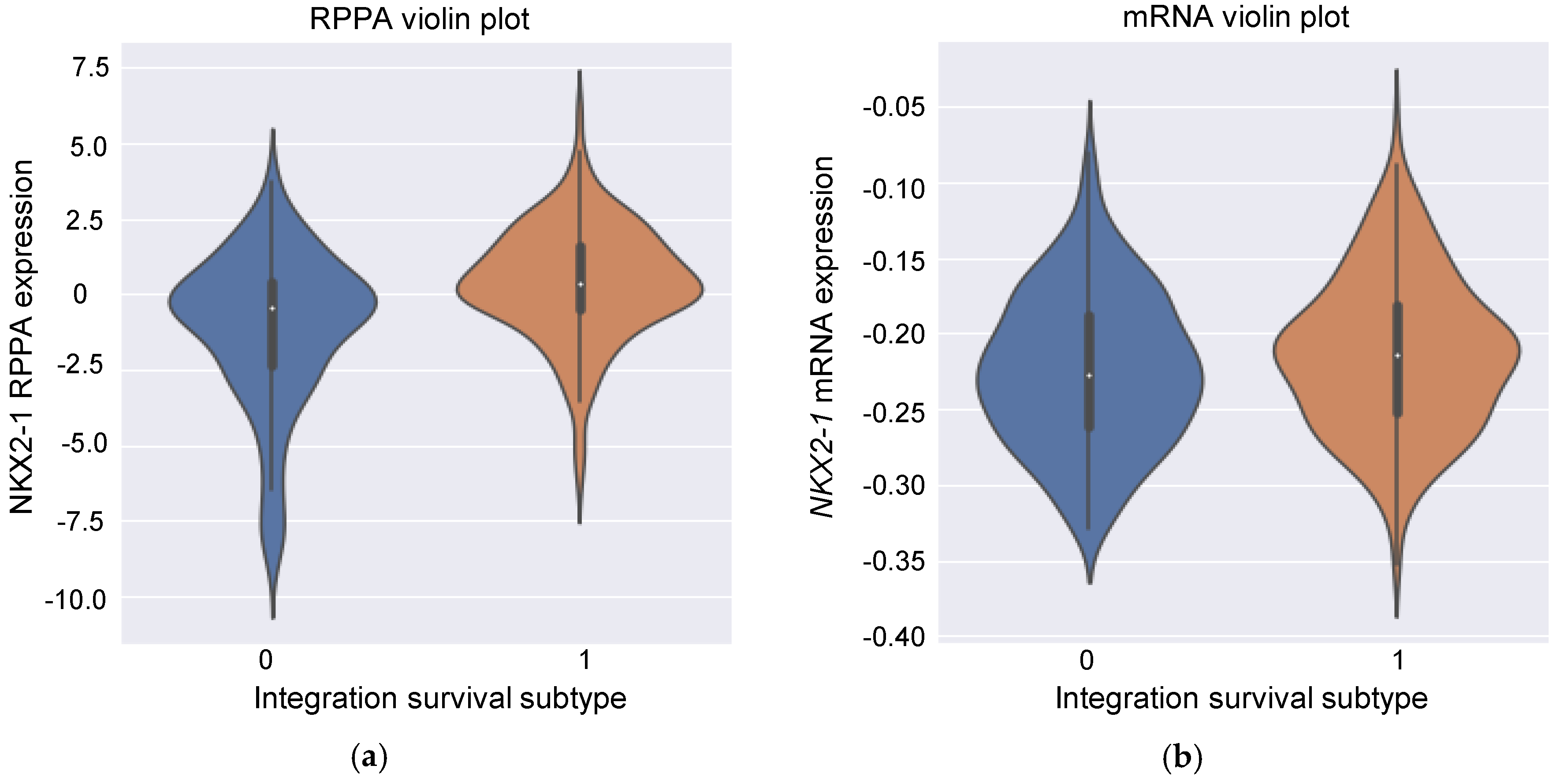
3.5. Insight into the Proteins Associated with Integration Survival Subtypes
4. Discussion
5. Conclusions
Supplementary Materials
Author Contributions
Funding
Acknowledgments
Conflicts of Interest
References
- Bray, F.; Ferlay, J.; Soerjomataram, I.; Siegel, R.L.; Torre, L.A.; Jemal, A. Global cancer statistics 2018: GLOBOCAN estimates of incidence and mortality worldwide for 36 cancers in 185 countries. CA Cancer J. Clin. 2018, 68, 394–424. [Google Scholar] [CrossRef] [Green Version]
- Siegel, R.L.; Miller, K.D.; Jemal, A. Cancer statistics, 2020. CA Cancer J. Clin. 2020, 70, 7–30. [Google Scholar] [CrossRef] [PubMed]
- Yamaguchi, T.; Nishiura, H. Predicting the Epidemiological Dynamics of Lung Cancer in Japan. J. Clin. Med. 2019, 8, 326. [Google Scholar] [CrossRef] [PubMed] [Green Version]
- Inamura, K. Lung Cancer: Understanding Its Molecular Pathology and the 2015 WHO Classification. Front. Oncol. 2017, 7, 193. [Google Scholar] [CrossRef] [Green Version]
- Cancer Genome Atlas Research Network. Comprehensive molecular profiling of lung adenocarcinoma. Nature 2014, 511, 543–550. [Google Scholar] [CrossRef] [PubMed]
- George, J.; Lim, J.S.; Jang, S.J.; Cun, Y.; Ozretic, L.; Kong, G.; Leenders, F.; Lu, X.; Fernandez-Cuesta, L.; Bosco, G.; et al. Comprehensive genomic profiles of small cell lung cancer. Nature 2015, 524, 47–53. [Google Scholar] [CrossRef]
- Cancer Genome Atlas Research Network. Comprehensive genomic characterization of squamous cell lung cancers. Nature 2012, 489, 519–525. [Google Scholar] [CrossRef]
- Wu, C.; Zhou, F.; Ren, J.; Li, X.; Jiang, Y.; Ma, S. A Selective Review of Multi-Level Omics Data Integration Using Variable Selection. High Throughput. 2019, 8, 4. [Google Scholar] [CrossRef] [Green Version]
- Ardila, D.; Kiraly, A.P.; Bharadwaj, S.; Choi, B.; Reicher, J.J.; Peng, L.; Tse, D.; Etemadi, M.; Ye, W.; Corrado, G.; et al. End-to-end lung cancer screening with three-dimensional deep learning on low-dose chest computed tomography. Nat. Med. 2019, 25, 954–961. [Google Scholar] [CrossRef]
- Xu, Y.; Hosny, A.; Zeleznik, R.; Parmar, C.; Coroller, T.; Franco, I.; Mak, R.H.; Aerts, H. Deep Learning Predicts Lung Cancer Treatment Response from Serial Medical Imaging. Clin. Cancer Res. 2019, 25, 3266–3275. [Google Scholar] [CrossRef] [Green Version]
- Ramazzotti, D.; Lal, A.; Wang, B.; Batzoglou, S.; Sidow, A. Multi-omic tumor data reveal diversity of molecular mechanisms that correlate with survival. Nat. Commun. 2018, 9, 4453. [Google Scholar] [CrossRef] [Green Version]
- Chaudhary, K.; Poirion, O.B.; Lu, L.; Garmire, L.X. Deep Learning-Based Multi-Omics Integration Robustly Predicts Survival in Liver Cancer. Clin. Cancer Res. 2018, 24, 1248–1259. [Google Scholar] [CrossRef] [Green Version]
- Asada, K.; Kobayashi, K.; Joutard, S.; Tubaki, M.; Takahashi, S.; Takasawa, K.; Komatsu, M.; Kaneko, S.; Sese, J.; Hamamoto, R. Uncovering Prognosis-Related Genes and Pathways by Multi-Omics Analysis in Lung Cancer. Biomolecules 2020, 10, 524. [Google Scholar] [CrossRef] [PubMed] [Green Version]
- Zhang, L.; Lv, C.; Jin, Y.; Cheng, G.; Fu, Y.; Yuan, D.; Tao, Y.; Guo, Y.; Ni, X.; Shi, T. Deep Learning-Based Multi-Omics Data Integration Reveals Two Prognostic Subtypes in High-Risk Neuroblastoma. Front. Genet. 2018, 9, 477. [Google Scholar] [CrossRef] [PubMed] [Green Version]
- Wei, L.; Jin, Z.; Yang, S.; Xu, Y.; Zhu, Y.; Ji, Y. TCGA-assembler 2: Software pipeline for retrieval and processing of TCGA/CPTAC data. Bioinformatics 2018, 34, 1615–1617. [Google Scholar] [CrossRef] [PubMed] [Green Version]
- Yuan, C.; Yang, H. Research on K-Value Selection Method of K-Means Clustering Algorithm. J. Multidiscip. Sci. J. 2019, 2, 226–253. [Google Scholar] [CrossRef] [Green Version]
- Calinski, T.; Harabasz, J. A dendrite method for cluster analysis. Commun. Stat. Theory Methods 1974, 3, 1–27. [Google Scholar] [CrossRef]
- Rousseeuw, P.J. Silhouettes: A graphical aid to the interpretation and validation of cluster analysis. J. Comput. Appl. Math. 1987, 20, 13. [Google Scholar] [CrossRef] [Green Version]
- van der Maaten, L.; Hinton, G. Visualizing Data using t-SNE. J. Mach. Learn. Res. 2008, 9, 7. [Google Scholar]
- Chen, T.; Guestrin, C. XGBoost: A Scalable Tree Boosting System. arXiv 2016, arXiv:1603.02754. [Google Scholar]
- Ke, G.; Meng, Q.; Finley, T.; Wang, T.; Chen, W.; Ma, W.; Ye, Q.; Liu, T.Y. LightGBM: A highly efficient gradient boosting decision tree. In Proceedings of the NIPS’17: 31st International Conference on Neural Information Processing Systems 2017, Long Beach, CA, USA, 4–9 December 2017; pp. 3149–3157. [Google Scholar]
- Lundberg, S.M.; Lee, S.I. A unified approach to interpreting model predictions. arXiv 2017, arXiv:1705.07874. [Google Scholar]
- Yang, L.; Lin, M.; Ruan, W.J.; Dong, L.L.; Chen, E.G.; Wu, X.H.; Ying, K.J. Nkx2-1: A novel tumor biomarker of lung cancer. J. Zhejiang Univ. Sci. B 2012, 13, 855–866. [Google Scholar] [CrossRef] [Green Version]
- Shi, Y.B.; Li, J.; Lai, X.N.; Jiang, R.; Zhao, R.C.; Xiong, L.X. Multifaceted Roles of Caveolin-1 in Lung Cancer: A New Investigation Focused on Tumor Occurrence, Development and Therapy. Cancers 2020, 12, 291. [Google Scholar] [CrossRef] [PubMed] [Green Version]
- Guo, T.; Kong, J.; Liu, Y.; Li, Z.; Xia, J.; Zhang, Y.; Zhao, S.; Li, F.; Li, J.; Gu, C. Transcriptional activation of NANOG by YBX1 promotes lung cancer stem-like properties and metastasis. Biochem. Biophys. Res. Commun. 2017, 487, 153–159. [Google Scholar] [CrossRef]
- Wang, J.; Deng, L.; Huang, J.; Cai, R.; Zhu, X.; Liu, F.; Wang, Q.; Zhang, J.; Zheng, Y. High expression of Fibronectin 1 suppresses apoptosis through the NF-kappaB pathway and is associated with migration in nasopharyngeal carcinoma. Am. J. Transl. Res. 2017, 9, 4502–4511. [Google Scholar]
- Kumara, H.; Bellini, G.A.; Caballero, O.L.; Herath, S.A.C.; Su, T.; Ahmed, A.; Njoh, L.; Cekic, V.; Whelan, R.L. P-Cadherin (CDH3) is overexpressed in colorectal tumors and has potential as a serum marker for colorectal cancer monitoring. Oncoscience 2017, 4, 139–147. [Google Scholar] [CrossRef] [Green Version]
- Taniuchi, K.; Nakagawa, H.; Hosokawa, M.; Nakamura, T.; Eguchi, H.; Ohigashi, H.; Ishikawa, O.; Katagiri, T.; Nakamura, Y. Overexpressed P-cadherin/CDH3 promotes motility of pancreatic cancer cells by interacting with p120ctn and activating rho-family GTPases. Cancer Res. 2005, 65, 3092–3099. [Google Scholar] [CrossRef] [PubMed] [Green Version]
- Gao, W.; Liu, Y.; Qin, R.; Liu, D.; Feng, Q. Silence of fibronectin 1 increases cisplatin sensitivity of non-small cell lung cancer cell line. Biochem. Biophys. Res. Commun. 2016, 476, 35–41. [Google Scholar] [CrossRef] [PubMed]
- Vieira, A.F.; Paredes, J. P-cadherin and the journey to cancer metastasis. Mol. Cancer 2015, 14, 178. [Google Scholar] [CrossRef] [Green Version]
- Wang, C.L.; Yue, D.S.; Zhang, Z.F.; Zhan, Z.L.; Sun, L.N. Value of thyroid transcription factor-1 in identification of the prognosis of bronchioloalveolar carcinoma. Zhonghua Yi Xue Za Zhi 2007, 87, 2350–2354. [Google Scholar] [CrossRef] [Green Version]
- Barletta, J.A.; Perner, S.; Iafrate, A.J.; Yeap, B.Y.; Weir, B.A.; Johnson, L.A.; Johnson, B.E.; Meyerson, M.; Rubin, M.A.; Travis, W.D.; et al. Clinical significance of TTF-1 protein expression and TTF-1 gene amplification in lung adenocarcinoma. J. Cell Mol. Med. 2009, 13, 1977–1986. [Google Scholar] [CrossRef] [PubMed]
- Han, X.; Tan, Q.; Yang, S.; Li, J.; Xu, J.; Hao, X.; Hu, X.; Xing, P.; Liu, Y.; Lin, L.; et al. Comprehensive Profiling of Gene Copy Number Alterations Predicts Patient Prognosis in Resected Stages I-III Lung Adenocarcinoma. Front. Oncol. 2019, 9, 556. [Google Scholar] [CrossRef] [PubMed] [Green Version]
- Au, N.H.; Cheang, M.; Huntsman, D.G.; Yorida, E.; Coldman, A.; Elliott, W.M.; Bebb, G.; Flint, J.; English, J.; Gilks, C.B.; et al. Evaluation of immunohistochemical markers in non-small cell lung cancer by unsupervised hierarchical clustering analysis: A tissue microarray study of 284 cases and 18 markers. J. Pathol. 2004, 204, 101–109. [Google Scholar] [CrossRef] [PubMed]
- Shah, L.; Walter, K.L.; Borczuk, A.C.; Kawut, S.M.; Sonett, J.R.; Gorenstein, L.A.; Ginsburg, M.E.; Steinglass, K.M.; Powell, C.A. Expression of syndecan-1 and expression of epidermal growth factor receptor are associated with survival in patients with nonsmall cell lung carcinoma. Cancer 2004, 101, 1632–1638. [Google Scholar] [CrossRef]
- Haque, A.K.; Syed, S.; Lele, S.M.; Freeman, D.H.; Adegboyega, P.A. Immunohistochemical study of thyroid transcription factor-1 and HER2/neu in non-small cell lung cancer: Strong thyroid transcription factor-1 expression predicts better survival. Appl. Immunohistochem. Mol. Morphol. 2002, 10, 103–109. [Google Scholar] [CrossRef]
- Pelosi, G.; Fraggetta, F.; Pasini, F.; Maisonneuve, P.; Sonzogni, A.; Iannucci, A.; Terzi, A.; Bresaola, E.; Valduga, F.; Lupo, C.; et al. Immunoreactivity for thyroid transcription factor-1 in stage I non-small cell carcinomas of the lung. Am. J. Surg. Pathol. 2001, 25, 363–372. [Google Scholar] [CrossRef]
- Barlesi, F.; Pinot, D.; Legoffic, A.; Doddoli, C.; Chetaille, B.; Torre, J.P.; Astoul, P. Positive thyroid transcription factor 1 staining strongly correlates with survival of patients with adenocarcinoma of the lung. Br. J. Cancer 2005, 93, 450–452. [Google Scholar] [CrossRef] [Green Version]
- Puglisi, F.; Barbone, F.; Damante, G.; Bruckbauer, M.; Di Lauro, V.; Beltrami, C.A.; Di Loreto, C. Prognostic value of thyroid transcription factor-1 in primary, resected, non-small cell lung carcinoma. Mod. Pathol. 1999, 12, 318–324. [Google Scholar]
- Stenhouse, G.; Fyfe, N.; King, G.; Chapman, A.; Kerr, K.M. Thyroid transcription factor 1 in pulmonary adenocarcinoma. J. Clin. Pathol. 2004, 57, 383–387. [Google Scholar] [CrossRef]
- Berghmans, T.; Paesmans, M.; Mascaux, C.; Martin, B.; Meert, A.P.; Haller, A.; Lafitte, J.J.; Sculier, J.P. Thyroid transcription factor 1—A new prognostic factor in lung cancer: A meta-analysis. Ann. Oncol. 2006, 17, 1673–1676. [Google Scholar] [CrossRef]
- Myong, N.H. Thyroid transcription factor-1 (TTF-1) expression in human lung carcinomas: Its prognostic implication and relationship with wxpressions of p53 and Ki-67 proteins. J. Korean Med. Sci. 2003, 18, 494–500. [Google Scholar] [CrossRef]
- Tan, D.; Li, Q.; Deeb, G.; Ramnath, N.; Slocum, H.K.; Brooks, J.; Cheney, R.; Wiseman, S.; Anderson, T.; Loewen, G. Thyroid transcription factor-1 expression prevalence and its clinical implications in non-small cell lung cancer: A high-throughput tissue microarray and immunohistochemistry study. Hum. Pathol. 2003, 34, 597–604. [Google Scholar] [CrossRef]
- Yoon, S.O.; Kim, Y.T.; Jung, K.C.; Jeon, Y.K.; Kim, B.H.; Kim, C.W. TTF-1 mRNA-positive circulating tumor cells in the peripheral blood predict poor prognosis in surgically resected non-small cell lung cancer patients. Lung Cancer 2011, 71, 209–216. [Google Scholar] [CrossRef] [PubMed]
- Liu, Y.; Beyer, A.; Aebersold, R. On the Dependency of Cellular Protein Levels on mRNA Abundance. Cell 2016, 165, 535–550. [Google Scholar] [CrossRef] [Green Version]
- Diao, G.; Vidyashankar, A.N. Assessing genome-wide statistical significance for large p small n problems. Genetics 2013, 194, 781–783. [Google Scholar] [CrossRef] [PubMed] [Green Version]
- Hamamoto, R.; Komatsu, M.; Takasawa, K.; Asada, K.; Kaneko, S. Epigenetics Analysis and Integrated Analysis of Multiomics Data, Including Epigenetic Data, Using Artificial Intelligence in the Era of Precision Medicine. Biomolecules 2019, 10, 62. [Google Scholar] [CrossRef] [Green Version]
- Chakraborty, S.; Tomsett, R.; Raghavendra, R.; Harborne, D.; Alzantot, M.; Cerutti, F.; Srivastava, M.B.; Preece, A.D.; Julier, S.J.; Rao, R.M.; et al. Interpretability of deep learning models: A survey of results. In 2017 IEEE SmartWorld, Ubiquitous Intelligence Computing, Advanced Trusted Computed, Scalable Computing Communications, Cloud Big Data Computing, Internet of People and Smart City Innovation, Proceedings of the 2017 IEEE SmartWorld, San Francisco, CA, USA, 4–8 August 2017; IEEE: New York, NY, USA, 2017; pp. 1–6. [Google Scholar] [CrossRef]


| The Number of Samples of Each Data Type | |||
|---|---|---|---|
| Data Name | LUAD | LUSC | Total |
| Common | 278 | 205 | 483 |
| Clinical_uncommon | 197 | 262 | 459 |
| mRNA_uncommon | 190 | 262 | 452 |
| miRNA_uncommon | 125 | 103 | 228 |
| RPPA_uncommon | 54 | 93 | 147 |
| CNV_uncommon | 190 | 259 | 449 |
| Somatic mutation_uncommon | 193 | 249 | 442 |
| Methylation_uncommon | 135 | 131 | 266 |
| The Number of Features in Each Step | |||
|---|---|---|---|
| Data Type | Before Compression | After Compression by Autoencoder | After Feature Selection by Cox-PH |
| mRNA | 13,049 | 100 | 12 |
| miRNA | 217 | 100 | 3 |
| RPPA | 150 | 100 | 3 |
| CNV | 14,786 | 100 | 5 |
| Somatic mutation | 18,977 | 100 | 3 |
| Methylation | 19,899 | 100 | 3 |
| Data Type | AUC |
|---|---|
| mRNA | 0.57 ± 0.05 |
| miRNA | 0.61 ± 0.07 |
| RPPA | 0.99 ± 0.00 |
| CNV | 0.43 ± 0.04 |
| Somatic mutation | 0.50 ± 0.07 |
| Methylation | 0.55 ± 0.05 |
Publisher’s Note: MDPI stays neutral with regard to jurisdictional claims in published maps and institutional affiliations. |
© 2020 by the authors. Licensee MDPI, Basel, Switzerland. This article is an open access article distributed under the terms and conditions of the Creative Commons Attribution (CC BY) license (http://creativecommons.org/licenses/by/4.0/).
Share and Cite
Takahashi, S.; Asada, K.; Takasawa, K.; Shimoyama, R.; Sakai, A.; Bolatkan, A.; Shinkai, N.; Kobayashi, K.; Komatsu, M.; Kaneko, S.; et al. Predicting Deep Learning Based Multi-Omics Parallel Integration Survival Subtypes in Lung Cancer Using Reverse Phase Protein Array Data. Biomolecules 2020, 10, 1460. https://0-doi-org.brum.beds.ac.uk/10.3390/biom10101460
Takahashi S, Asada K, Takasawa K, Shimoyama R, Sakai A, Bolatkan A, Shinkai N, Kobayashi K, Komatsu M, Kaneko S, et al. Predicting Deep Learning Based Multi-Omics Parallel Integration Survival Subtypes in Lung Cancer Using Reverse Phase Protein Array Data. Biomolecules. 2020; 10(10):1460. https://0-doi-org.brum.beds.ac.uk/10.3390/biom10101460
Chicago/Turabian StyleTakahashi, Satoshi, Ken Asada, Ken Takasawa, Ryo Shimoyama, Akira Sakai, Amina Bolatkan, Norio Shinkai, Kazuma Kobayashi, Masaaki Komatsu, Syuzo Kaneko, and et al. 2020. "Predicting Deep Learning Based Multi-Omics Parallel Integration Survival Subtypes in Lung Cancer Using Reverse Phase Protein Array Data" Biomolecules 10, no. 10: 1460. https://0-doi-org.brum.beds.ac.uk/10.3390/biom10101460