Dynamic Modeling of Planar Multi-Link Flexible Manipulators

Abstract

A closed-form dynamic model of the planar multi-link flexible manipulator is presented. The assumed modes method is used with the Lagrangian formulation to obtain the dynamic equations of motion. Explicit equations of motion are derived for a three-link case assuming two modes of vibration for each link. The eigenvalue problem associated with the mass boundary conditions, which changes with the robot configuration and payload, is discussed. The time-domain simulation results and frequency-domain analysis of the dynamic model are presented to show the validity of the theoretical derivation.

1. Introduction

The use of lightweight materials and the long or slender design of manipulators introduce link flexibility. Neglecting this during the modeling and control design of flexible link manipulators (FLMs) causes static steady-state and dynamic tracking and vibration errors. Lightweight flexible arms have many advantages over rigid body robots such as high payload-to-weight ratio, smaller actuators, and safer operation (due to reduced inertia) because of which they can be used in many engineering applications such as construction automation, robotic surgery, aerospace industry, and space research [1]. Some applications require the design of long and slender mechanical structures which possess some degrees of in-built flexibility because of the material used and the length of the link. Moreover, the use of lighter arms and cheaper gears by robot manufacturers is justifiable in order to compete with lower prices of the manipulators in recent years. However, the link flexibility causes deflection of the links and unwanted oscillations leading to problems in precise position control of the end-effector. To fully use the lightweight flexible manipulators, the problem of oscillations must be properly addressed by designing a suitable control algorithm to reduce the vibration of the end-effector to an acceptable range depending on the application.

The highly nonlinear dynamics of the FLMs with an infinite number of degrees of freedom (DoFs) make their control more complicated compared to the conventional industrial robot. An accurate model of the system aids in the development of efficient and optimal model-based control algorithms for the FLMs. In this context, it is desirable to build a mathematical model of the system incorporating flexible link dynamics in an accurate and computationally affordable way. The complexity associated with the modeling of link flexibility in FLMs with infinite DoFs must be addressed by describing the system with finite DoFs and still being able to represent all the dynamically relevant properties of the actual system such as flexibility effects, dynamic interactions, and coupling effects. There are different models of the flexible bodies available in the literature depending upon the assumptions, model complexity, and accuracy. The accuracy of the models depends on the assumptions made to simplify the complexity of the FLM system. The major approaches of modeling flexible bodies include lumped parameter method (LPM), finite element method (FEM), transfer matrix method (TMM), and assumed modes method (AMM). Apart from these methods, there are many other methods that are used for obtaining the dynamic model of the FLMs which include, but are not limited to, perturbation method, pseudo-rigid body method, global mode method, and modal integration method [1].

In LPM, the link flexibility is modeled by a set of mass, spring, and damper connected in series. Although LPM is simple and easy to implement, there is difficulty in determining the spring constant accurately. In FEM, the flexible link is modeled as a combination of a finite number of elements interconnected at nodes, and the displacement at any point of the continuous element is expressed in terms of the finite number of displacements at the nodal points multiplied by the polynomial interpolation functions [2]. The FEM is applicable for complex structures and can handle nonlinear and mixed boundary conditions, but it is computationally expensive because of a large number of state-space equations. In TMM, each element of the system is represented by a transfer matrix that transfers a state vector from one end of the element to the other, and the individual element matrices are multiplied together to obtain the system transfer matrix [3]. The TMM is a frequency-domain technique but it is difficult to include the interaction between the gross motion and the flexible dynamics of the manipulator [4].

Among different modeling methods, AMM is more widely used in the literature. AMM has been used by many researchers to develop a dynamic model of flexible mechanical systems and verified experimentally [5,6,7,8]. In this method, the link flexibility is represented by a combination of spatial mode shapes and time-varying generalized coordinates. The modal series is truncated to a finite dimension based on the fact that the dynamics and overall motion of the links are dominantly governed by the first few low-frequency modes [4]. The choice of proper boundary conditions is important while using AMM for modeling FLMs. It is also equally important to select compatible joint variables, deflection variables, and their corresponding mode shapes functions [9,10]. Four applicable boundary conditions according to the general beam vibration theories, pinned-pinned, clamped-pinned, clamped-free, and clamped-clamped, are detailed in [11,12].

The finite element discretization of the flexible bodies introduces a large number of DoFs which causes the simulation of the multibody system computationally expensive. Therefore, model reduction is a necessary procedure for reducing the elastic DoFs to allow an efficient simulation of the multibody system while keeping an accurate description of the predominant dynamic behavior. Model reduction involves a trade-off between the model order and the accuracy of representing the real plant dynamics by the model. In other words, the order of the dynamic model should such that it is suitable to be used for real-time control and at the same time should not lead to a spill-over effect (the problem of un-modeled residual modes) that destabilizes the system. Various model reduction techniques have been developed in the literature which can be divided into three main categories: 1. Static condensation, substructuring, and modal truncation (Guyan reduction, dynamic reduction, component mode synthesis, improved reduction system method, and system equivalent expansion reduction process), 2. Padé and Padé-type approximations (Krylov subspace method), and 3. Balancing-related truncation techniques [13,14]. The Craig-Bampton method (component mode synthesis technique) is one of the most often applied methods for the reduction of mechanical systems [15]. The quality of the reduced models depends on the selection of the right modes in complex systems, which needs an experienced user.

In the AMM, the reduced-order dynamic model is obtained by omitting the higher frequency system dynamics from the model. It is based on the assumptions that the modes of higher frequency, omitted from the reduced-order model, have little effect on the performance of the manipulator system, as they contain little energy compared with the retained modes [8]. In this way, it is reasonable to reduce the number of vibration modes to a small finite number for obtaining the reduced-order model suitable for real-time control. Other justifications for retaining fewer modes in the model are based on the low amplitudes of high-frequency terms that are dropped and the fact that the actuators and sensors cannot operate in the high-frequency range. However, the higher modes should be included in the model if it is likely that these modes may excite the servo-loop frequencies [2]. Although FEM with more DoFs yields more precise results than AMM, AMM is preferred to FEM for real-time control purposes [16].

Accurate dynamic modeling of FLMs is of ongoing interest for researchers worldwide. The Equivalent Rigid-Link System (ERLS) approach for 3-D FLM has been developed in [17] through FEM and component mode synthesis techniques. Hamilton’s principle is applied in [16] to obtain the dynamic model of a single-link flexible manipulator stiffened with cables. In [18], AMM is used in conjunction with recursive Gibbs-Appell formulation to obtain the dynamic model of flexible cooperative mobile manipulators that are kinematically and dynamically constrained. Explicit dynamic models of the one-link flexible arm [19,20,21,22,23,24,25,26,27] and the two-link flexible arm [6,28,29,30,31,32,33] have been derived and methods to obtain the mathematical model of a general n-link flexible arm [6] have been formulated based on AMM.

The research in the field of FLMs is more concentrated with the one-link, and two-link flexible manipulators than with the FLMs with more than two links. Although various formulations have been proposed for general dynamic modeling of multi-link flexible manipulators, an explicit model of manipulators with more than two links has not been well-studied in the literature. The issue about the mode shapes and eigenfrequencies variation with the robot configuration becomes more prominent for the arm with more than one link. In most of the studies that are based on the AMM, the effects of robot configurations on the mode shapes and eigenfrequencies have been ignored.

The aim of this work is to derive a dynamic model of the planar multi-link flexible manipulator using the AMM and discuss the eigenvalue problem associated with the mass boundary conditions, which changes with the robot configuration and payload. The Lagrangian method is used to derive the equations of motion, where the links are modeled as Euler-Bernoulli beams satisfying clamped-mass boundary conditions. The authors in [6] have discussed the problem of time-varying mass boundary conditions for the first link in the two-link arm. This paper further explores this problem for a three-link case. The effects of robot configurations on the mode shapes and frequencies are discussed in detail. The time-domain simulation results and frequency-domain analysis of the dynamic model of the planar three-link flexible manipulator are presented. The benefits of including passive structural damping in the simulation model are discussed.

The paper is organized into five sections as follows. Section 2 describes the kinematic relationships and the dynamic model for a multi-link planar manipulator using the AMM and Lagrangian formulation. Section 3 presents a dynamic model of a three-link planar flexible manipulator assuming two mode shapes for each link. The simulation results are reported in Section 4. Conclusions and discussions follow in Section 5.

2. Modeling

2.1. Kinematics

Consider a planar n-link flexible serial manipulator with n revolute joints. The following assumptions are made for the development of the dynamic model of the manipulator.

• Each link of the manipulator can undergo bending deformations (transversal deflection) in the plane of motion.
• The torsional effects and shear deformations are neglected.
• All joints are rigid and revolute. This assumption is considered because of higher joint stiffness compared to link stiffness.
• Link deflections are small.

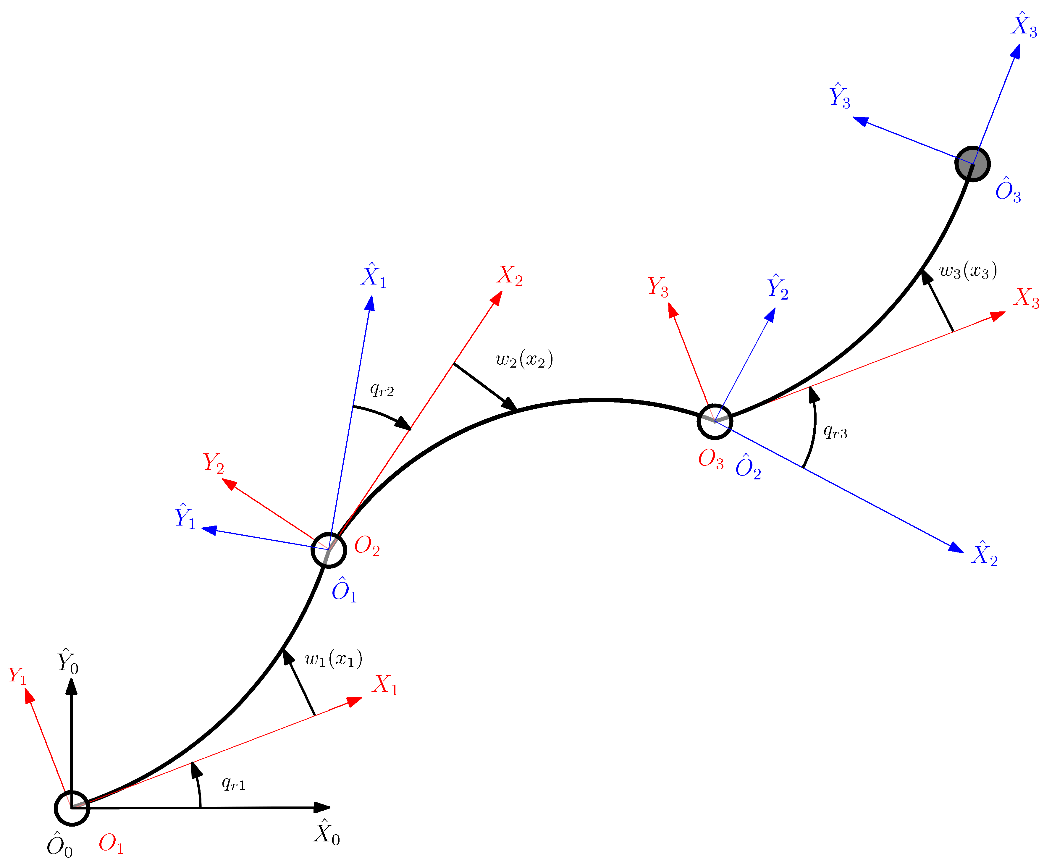
Figure 1 shows a model of a planar three-link flexible manipulator. The direct kinematic model of the planar manipulator can be formulated in terms of displacement vectors and rotation matrices. The coordinate frames for the manipulator are assigned following a methodology similar to the Denavit-Hartenberg convention: the inertial frame (${\widehat{X}}_0,{\widehat{Y}}_0$), the rigid body moving frame associated to link i ($X_i,Y_i$) located at joint i, and the flexible body moving frame associated to link i (${\widehat{X}}_i,{\widehat{Y}}_i$) located at the tip of link i. The rigid motion of link i is represented by the joint i position $q_{ri}$, and the deflection at any point $x_i$ along the link i is described by $w_i\left(x_i\right)$, where $0\le x_i\le {\ell }_i$, and ${\ell }_i$ is the length of the link i.

The position of a point along the link i and its endpoint referred to frame ($X_i,Y_i$) are given by Equations (1) and (2) respectively. Here, ${}^i{\mathit{r}}_{i+1}$ also denotes the position of the origin of frame ($X_{i+1},Y_{i+1}$) with respect to frame ($X_i,Y_i$). The absolute positions of the aforementioned points referred to frame (${\widehat{X}}_0,{\widehat{Y}}_0$) are given by Equations (3) and (4) respectively, where ${\mathit{W}}_i$ is the cumulative transformation from inertial frame (${\widehat{X}}_0,{\widehat{Y}}_0$) to frame ($X_i,Y_i$). ${\mathit{W}}_i$ can be calculated recursively using Equations (5)–(7), where ${\mathit{A}}_i$ represents the joint rotation matrix, and ${\mathit{E}}_{i-1}$ represents the influence of the elastic deformation of the previous link $i-1$ in the orientation of link i. The orientations of frames ($X_i,Y_i$) and (${\widehat{X}}_{i-1},{\widehat{Y}}_{i-1}$) with respect to frame (${\widehat{X}}_0,{\widehat{Y}}_0$) are given by Equations (8) and (9) respectively.

$$\begin{array}{cc}\hfill {}^i{\mathit{p}}_i& ={\left[\begin{array}{cc}{x}_i& w_i\left(x_i\right)\end{array}\right]}^T\hfill \end{array}$$

(1)

$$\begin{array}{cc}\hfill {}^i{\mathit{r}}_{i+1}& ={\left.{}^i{\mathit{p}}_i\right|}_{x_i={\ell }_i}={\left[\begin{array}{cc}{\ell }_i& w_{ie}\end{array}\right]}^T\hfill \end{array}$$

(2)

$$\begin{array}{cc}\hfill {\mathit{p}}_i& ={\mathit{r}}_i+{\mathit{W}}_i^i{\mathit{p}}_i\hfill \end{array}$$

(3)

$$\begin{array}{cc}\hfill {\mathit{r}}_{i+1}& ={\mathit{r}}_i+{\mathit{W}}_i^i{\mathit{r}}_{i+1}\hfill \end{array}$$

(4)

$$\begin{array}{cc}\hfill {\mathit{W}}_i& ={\mathit{W}}_{i-1}{\mathit{E}}_{i-1}{\mathit{A}}_i={\widehat{\mathit{W}}}_{i-1}{\mathit{A}}_i,{\mathit{W}}_0={\widehat{\mathit{W}}}_0=\mathit{I}\hfill \end{array}$$

(5)

$$\begin{array}{cc}\hfill {\mathit{A}}_i& =\left[\begin{array}{cc}cos\left(q_i\right)& -sin\left(q_i\right)\\ sin\left(q_i\right)& cos\left(q_i\right)\end{array}\right]\hfill \end{array}$$

(6)

$$\begin{array}{cc}\hfill {\mathit{E}}_i& =\left[\begin{array}{cc}1& -w_{ie}^{\prime }\\ w_{ie}^{\prime }& 1\end{array}\right],w_{ie}^{\prime }={\left.\frac{\partial w_i\left(x_i\right)}{\partial x_i}\right|}_{x_i={\ell }_i},{\mathit{E}}_0=\mathit{I}\hfill \end{array}$$

(7)

$$\begin{array}{cc}\hfill {\alpha }_i& =\sum _{j=1}^i{q}_{rj}+\sum _{k=1}^{i-1}{w}_{ke}^{\prime },i\le n\hfill \end{array}$$

(8)

$$\begin{array}{cc}\hfill {\widehat{\alpha }}_i& =\sum _{j=1}^{i-1}{q}_{rj}+\sum _{k=1}^{i-1}{w}_{ke}^{\prime },i\le n+1\hfill \end{array}$$

(9)

The differential kinematics can be obtained using the time derivatives of the displacement and rotation as shown in Equations (10)–(19).

$$\begin{array}{cc}\hfill {}^i{\dot{\mathit{p}}}_i& ={\left[\begin{array}{cc}0& {\dot{w}}_i\end{array}\right]}^T\hfill \end{array}$$

(10)

$$\begin{array}{cc}\hfill {}^i{\dot{\mathit{r}}}_{i+1}& ={\left.{}^i{\dot{\mathit{p}}}_i\right|}_{x_i={\ell }_i}={\left[\begin{array}{cc}0& {\dot{w}}_{ie}\end{array}\right]}^T\hfill \end{array}$$

(11)

$$\begin{array}{cc}\hfill {\dot{\mathit{p}}}_i& ={\dot{\mathit{r}}}_i+{\dot{\mathit{W}}}_i^i{p}_i+{\mathit{W}}_i^i{\dot{\mathit{p}}}_i\hfill \end{array}$$

(12)

$$\begin{array}{cc}\hfill {\dot{\mathit{r}}}_{i+1}& ={\dot{\mathit{r}}}_i+{\dot{\mathit{W}}}_i^i{r}_{i+1}+{\mathit{W}}_i^i{\dot{\mathit{r}}}_{i+1}\hfill \end{array}$$

(13)

$$\begin{array}{cc}\hfill {\dot{\alpha }}_i& =\sum _{j=1}^i{\dot{q}}_j+\sum _{k=1}^{i-1}{\dot{w}}_{ke}^{\prime }\hfill \end{array}$$

(14)

$$\begin{array}{cc}\hfill {\dot{\widehat{\alpha }}}_i& =\sum _{j=1}^{i-1}{\dot{q}}_j+\sum _{k=1}^{i-1}{\dot{w}}_{ke}^{\prime }\hfill \end{array}$$

(15)

$$\begin{array}{cc}\hfill {\dot{\mathit{A}}}_i& =\mathit{S}{\mathit{A}}_i\dot{q_i},\mathit{S}=\left[\begin{array}{cc}0& -1\\ 1& 0\end{array}\right]\hfill \end{array}$$

(16)

$$\begin{array}{cc}\hfill {\dot{\mathit{E}}}_i& =\mathit{S}{\dot{w}}_{ie}^{\prime }\hfill \end{array}$$

(17)

$$\begin{array}{cc}\hfill {\dot{\mathit{W}}}_i& ={\dot{\widehat{\mathit{W}}}}_{i-1}{\mathit{A}}_i+{\widehat{\mathit{W}}}_{i-1}{\dot{\mathit{A}}}_i\hfill \end{array}$$

(18)

$$\begin{array}{cc}\hfill {\dot{\widehat{\mathit{W}}}}_{i-1}& ={\dot{\mathit{W}}}_{i-1}{\mathit{E}}_{i-1}+{\mathit{W}}_{i-1}{\dot{\mathit{E}}}_{i-1}\hfill \end{array}$$

(19)

2.2. Assumed Modes Method

Flexible Links of the manipulator are modeled as Euler-Bernoulli beams of uniform density (mass per unit length) ${\rho }_i$ and constant flexural rigidity ${\left(EI\right)}_i$. The elastic deformation $w_i(x_i,t)$ of Euler-Bernoulli beam at time t satisfies the partial differential equation given by Equation (20), where $c_i=\sqrt{\frac{EI}{{\rho }_i}}$ [6].

$$c_i^2\frac{{\partial }^4{w}_i(x_i,t)}{\partial x_i^4}+\frac{{\partial }^2{w}_i(x_i,t)}{\partial t^2}=0,i=1,\cdots ,n$$

(20)

Equation (20) can be solved by imposing proper boundary conditions at the base and the end of each link. Clamped boundary condition at the base of each link (assuming that the closed feedback control loop around the joint enforces the clamped assumptions [6]) is given by Equations (21) and (22).

$${\left.w_i(x_i,t)\right|}_{x_i=0}=0,i=1,\cdots ,n$$

(21)

$${\left.\frac{\partial w_i(x_i,t)}{\partial x_i}\right|}_{x_i=0}=0,i=1,\cdots ,n$$

(22)

Assuming that the tip of each link is free of the dynamic constraints, the mass boundary conditions presented in [6,28] are used in this paper which are given by Equations (23) and (24), where $J_{Di}$ is the moment of inertia at the end of the link i, $m_{Di}$ is the actual mass at the end of the link i, and $M_{Di}$ accounts for the contributions of the masses of the distal links, hubs, and payloads non-collocated at the end of the link i, weighted by the relative distance from the axis $Y_i$ (shearing axis at the end of link i) [6]. The contribution of $M_{Di}$ is not included in the mode shape analysis in [6,28]. In this paper, the contribution of $M_{Di}$ is considered along with the effect of robot configurations while calculating $J_{Di}$. The values of $M_{Di}$ and $J_{Di}$ are evaluated in correspondence to the unreformed configuration.

$$\begin{array}{cc}\hfill {\left(EI\right)}_i{\left.\frac{{\partial }^2{w}_i(x_i,t)}{\partial x_i^2}\right|}_{x_i={\ell }_i}& =-J_{Di}\frac{d^2}{d{t}^2}\left({\left.\frac{\partial w_i(x_i,t)}{\partial x_i}\right|}_{x_i={\ell }_i}\right)-M_{Di}\frac{d^2}{d{t}^2}\left({\left.w_i(x_i,t)\right|}_{x_i={\ell }_i}\right),i=1,\cdots ,n\hfill \end{array}$$

(23)

$$\begin{array}{cc}\hfill {\left(EI\right)}_i{\left.\frac{{\partial }^3{w}_i(x_i,t)}{\partial x_i^3}\right|}_{x_i={\ell }_i}& =m_{Di}\frac{d^2}{d{t}^2}\left({\left.w_i(x_i,t)\right|}_{x_i={\ell }_i}\right)+M_{Di}\frac{d^2}{d{t}^2}\left({\left.\frac{\partial w_i(x_i,t)}{\partial x_i}\right|}_{x_i={\ell }_i}\right),i=1,\cdots ,n\hfill \end{array}$$

(24)

Using AMM, the link deflection is expressed using a finite-dimensional model of order $n_f$ as shown in Equation (25), where $q_{fij}\left(t\right)$ is the time-varying variable related to the spatial assumed mode shape ${\varphi }_{ij}\left(x_i\right)$ of link i and mode of vibration j [6].

$$w_i(x_i,t)=\sum _{j=1}^{n_f}{\varphi }_{ij}\left(x_i\right)q_{fij}\left(t\right)$$

(25)

Using separation of variables, shown in Equation (25), the solution of Equation (20) can be written as Equation (26), where $a_{ij}={\omega }_{ij}^2$ is a positive constant, and ${\omega }_{ij}$ is the $j^{th}$ natural angular frequency of link i.

$$\frac{c_i^2}{{\varphi }_{ij}\left(x_i\right)}\frac{d^4{\varphi }_{ij}\left(x_i\right)}{d{x}_i^4}=-\frac{1}{q_{fij}\left(t\right)}\frac{d^2{q}_{fij}\left(t\right)}{d{t}^2}=a_{ij}={\omega }_{ij}^2$$

(26)

From Equation (26), the time harmonic function $q_{fij}\left(t\right)$ and the spatial assumed mode shapes ${\varphi }_{ij}\left(x_i\right)$ are given by Equations (27) and (28) respectively, where ${\beta }_{ij}$ is given by Equation (29).

$$q_{fij}\left(t\right)=e^{\sqrt{-1}{\omega }_{ij}^{2}t}$$

(27)

$$\begin{array}{cc}\hfill {\varphi }_{ij}\left(x_i\right)& =c_{1ij}sin\left({\beta }_{ij}{x}_i\right)+c_{2ij}cos\left({\beta }_{ij}{x}_i\right)+c_{3ij}sinh\left({\beta }_{ij}{x}_i\right)+c_{4ij}cosh\left({\beta }_{ij}{x}_i\right)\hfill \end{array}$$

(28)

$${\beta }_{ij}^4=\frac{{\omega }_{ij}^2}{c_i^2}=\frac{{\rho }_i{\omega }_{ij}^2}{EI}$$

(29)

Additionally, Equation (26) is rearranged to obtain Equation (30).

$$\begin{array}{c}\hfill \frac{{\ddot{q}}_{fij}\left(t\right)}{q_{fij}\left(t\right)}=-\frac{{\beta }_{ij}^4{\left(EI\right)}_i}{{\rho }_i}\end{array}$$

(30)

The values of $c_{1ij}$, $c_{2ij}$, $c_{3ij}$, $c_{4ij}$, and the natural frequencies ${\omega }_{ij}$ are calculated from the boundary conditions. The boundary conditions given by Equations (21) and (22) are modified according to the AMM as

$${\left.q_{fij}\left(t\right){\varphi }_{ij}\left(x_i\right)\right|}_{x_i=0}=0⟹{\left.{\varphi }_{ij}\left(x_i\right)\right|}_{x_i=0}=0,$$

(31)

$${\left.q_{fij}\left(t\right)\frac{\partial {\varphi }_{ij}\left(x_i\right)}{\partial x_i}\right|}_{x_i=0}=0⟹{\left.{\varphi }_{ij}^{\prime }\left(x_i\right)\right|}_{x_i=0}=0.$$

(32)

Similarly, the boundary conditions given by Equations (23) and (24) are modified according to the AMM as

$$\begin{array}{cc}\hfill {\left(EI\right)}_i{\left.{\varphi }_{ij}^{″}\left(x_i\right)\right|}_{x_i={\ell }_i}{q}_{fij}\left(t\right)& =-J_{Di}{\left.{\varphi }_{ij}^{\prime }\left(x_i\right)\right|}_{x_i={\ell }_i}{\ddot{q}}_{fij}\left(t\right)-M_{Di}{\left.{\varphi }_{ij}\left(x_i\right)\right|}_{x_i={\ell }_i}{\ddot{q}}_{fij}\left(t\right),\hfill \end{array}$$

(33)

$$\begin{array}{cc}\hfill {\left(EI\right)}_i{\left.{\varphi }_{ij}^{‴}\left(x_i\right)\right|}_{x_i={\ell }_i}{q}_{fij}\left(t\right)& =m_{Di}{\left.{\varphi }_{ij}\left(x_i\right)\right|}_{x_i={\ell }_i}{\ddot{q}}_{fij}\left(t\right)+M_{Di}{\left.{\varphi }_{ij}^{\prime }\left(x_i\right)\right|}_{x_i={\ell }_i}{\ddot{q}}_{fij}\left(t\right).\hfill \end{array}$$

(34)

Substituting Equation (30) in Equations (33) and (34), we get

$$\begin{array}{cc}\hfill {\left.{\varphi }_{ij}^{″}\left(x_i\right)\right|}_{x_i={\ell }_i}-\frac{{\beta }_{ij}^4}{{\rho }_i}\left[J_{Di}{\left.{\varphi }_{ij}^{\prime }\left(x_i\right)\right|}_{x_i={\ell }_i}\right.\left.+M_{Di}{\left.{\varphi }_{ij}\left(x_i\right)\right|}_{x_i={\ell }_i}\right]& =0,\hfill \end{array}$$

(35)

$$\begin{array}{cc}\hfill {\left.{\varphi }_{ij}^{‴}\left(x_i\right)\right|}_{x_i={\ell }_i}+\frac{{\beta }_{ij}^4}{{\rho }_i}\left[m_{Di}{\left.{\varphi }_{ij}\left(x_i\right)\right|}_{x_i={\ell }_i}\right.\left.+M_{Di}{\left.{\varphi }_{ij}^{\prime }\left(x_i\right)\right|}_{x_i={\ell }_i}\right]& =0.\hfill \end{array}$$

(36)

Substituting Equation (28) in Equations (31) and (32), we get

$$c_{3ij}=-c_{1ij},\mathrm{and}{c}_{4ij}=-c_{2ij}.$$

(37)

Similarly, substituting Equation (28) in Equations (35) and (36), we get a homogeneous system of equations of the form

$$\mathit{F}\left({\beta }_{ij}\right)\left[\begin{array}{c}{c}_{1ij}\\ c_{2ij}\end{array}\right]=\mathbf{0},\mathit{F}\left({\beta }_{ij}\right)=\left[\begin{array}{cc}{F}_{11}& F_{12}\\ F_{21}& F_{22}\end{array}\right],$$

(38)

$$\begin{array}{cc}\hfill F_{11}& ={\rho }_i[sin\left({\beta }_{ij}{\ell }_i\right)+sinh\left({\beta }_{ij}{\ell }_i\right)]+{\beta }_{ij}^2[M_{Di}(sin\left({\beta }_{ij}{\ell }_i\right)-sinh\left({\beta }_{ij}{\ell }_i\right))+J_{Di}{\beta }_{ij}(cos\left({\beta }_{ij}{\ell }_i\right)-cosh\left({\beta }_{ij}{\ell }_i\right))],\hfill \\ \hfill F_{12}& ={\rho }_i[cos\left({\beta }_{ij}{\ell }_i\right)+cosh\left({\beta }_{ij}{\ell }_i\right)]+{\beta }_{ij}^2[M_{Di}(cos\left({\beta }_{ij}{\ell }_i\right)-cosh\left({\beta }_{ij}{\ell }_i\right))-J_{Di}{\beta }_{ij}(sin\left({\beta }_{ij}{\ell }_i\right)+sinh\left({\beta }_{ij}{\ell }_i\right))],\hfill \\ \hfill F_{21}& ={\rho }_i[cos\left({\beta }_{ij}{\ell }_i\right)+cosh\left({\beta }_{ij}{\ell }_i\right)]-{\beta }_{ij}[m_{Di}(sin\left({\beta }_{ij}{\ell }_i\right)-sinh\left({\beta }_{ij}{\ell }_i\right))+M_{Di}{\beta }_{ij}(cos\left({\beta }_{ij}{\ell }_i\right)-cosh\left({\beta }_{ij}{\ell }_i\right))],\hfill \\ \hfill F_{22}& =-{\beta }_{ij}[m_{Di}[cos\left({\beta }_{ij}{\ell }_i\right)-cosh\left({\beta }_{ij}{\ell }_i\right)]-M_{Di}{\beta }_{ij}[sin\left({\beta }_{ij}{\ell }_i\right)+sinh\left({\beta }_{ij}{\ell }_i\right)]]-{\rho }_i[sin\left({\beta }_{ij}{\ell }_i\right)-sinh\left({\beta }_{ij}{\ell }_i\right)],\hfill \end{array}$$

where ${\beta }_{ij}$ for each link i and mode of vibration j is obtained from the nontrivial solution of Equation (38), i.e. $det\left(\mathit{F}\left({\beta }_{ij}\right)\right)=0$, which results into the transcendental equation given by Equation (39). The solutions ($n_f$ positive roots) of Equation (39) (${\beta }_{ij}\in [{\beta }_{i1}\cdots {\beta }_{i{n}_f}]$) are obtained numerically and the natural frequencies ${\omega }_{ij}$ are obtained using Equation (29). It can be noted that the values of ${\beta }_{ij}$ depends explicitly on $m_{Di}$, $J_{Di}$, and $M_{Di}$.

$$\begin{array}{c}\hfill {\rho }_i^2+{\rho }_i^{2}cos\left({\beta }_{ij}{\ell }_i\right)cosh\left({\beta }_{ij}{\ell }_i\right)+J_{Di}{\beta }_{ij}^4{m}_{Di}+M_{Di}^2{\beta }_{ij}^{4}cos\left({\beta }_{ij}{\ell }_i\right)cosh\left({\beta }_{ij}{\ell }_i\right)+{\beta }_{ij}{m}_{Di}{\rho }_{i}cos\left({\beta }_{ij}{\ell }_i\right)sinh\left({\beta }_{ij}{\ell }_i\right)=\\ \hfill =M_{Di}^2{\beta }_{ij}^4+{\beta }_{ij}{m}_{Di}{\rho }_{i}cosh\left({\beta }_{ij}{\ell }_i\right)sin\left({\beta }_{ij}{\ell }_i\right)+J_{Di}{\beta }_{ij}^4{m}_{Di}cos\left({\beta }_{ij}{\ell }_i\right)cosh\left({\beta }_{ij}{\ell }_i\right)+J_{Di}{\beta }_{ij}^3{\rho }_{i}cos\left({\beta }_{ij}{\ell }_i\right)sinh\left({\beta }_{ij}{\ell }_i\right)+\\ \hfill +J_{Di}{\beta }_{ij}^3{\rho }_{i}cosh\left({\beta }_{ij}{\ell }_i\right)sin\left({\beta }_{ij}{\ell }_i\right)+2M_{Di}{\beta }_{ij}^2{\rho }_{i}sin\left({\beta }_{ij}{\ell }_i\right)sinh\left({\beta }_{ij}{\ell }_i\right)\end{array}$$

(39)

The constants $c_{1ij}$ and $c_{2ij}$ are calculated by substituting the corresponding values of ${\beta }_{ij}$ in Equation (38) and scaled using the orthonormalization condition of the modes of vibration represented by Equation (40), where ${\delta }_{jk}$ is the Kronecker delta symbol, and $m_{\ell i}$ is the mass of link i.

$$\begin{array}{c}\hfill {\int }_0^{{\ell }_i}{\rho }_i{\varphi }_{ij}\left(x_i\right){\varphi }_{ik}\left(x_i\right)d{x}_i+m_{Di}{\varphi }_{ij}\left({\ell }_i\right){\varphi }_{ik}\left({\ell }_i\right)+M_{Di}{\varphi }_{ij}\left({\ell }_i\right){\varphi }_{ik}^{\prime }\left({\ell }_i\right)+J_{Di}{\varphi }_{ij}^{\prime }\left({\ell }_i\right){\varphi }_{ik}^{\prime }\left({\ell }_i\right)+M_{Di}{\varphi }_{ij}^{\prime }\left({\ell }_i\right){\varphi }_{ik}\left({\ell }_i\right)=m_{\ell i}{\delta }_{jk}\end{array}$$

(40)

2.3. Equations of Motion

Consider $m_{hi}$ is the mass of hub i, $m_p$ is the mass of payload, $J_{\ell i}$ is the inertia of link i about the axis at its center of mass, $J_{hi}$ is the inertia of hub i about the joint i axis, $J_p$ is the inertia of the payload about the axis at its center of mass, $d_{\ell ij}$ is the distance of the center of mass of link i from joint j axis, $d_{hij}$ is the distance of the center of mass of hub i from joint j axis, and $d_{pj}$ is the distance of the center of mass of the payload from the joint j axis.

The equations of motion of a planar n-link manipulator can be derived using the Lagrangian method. The total kinetic energy of the manipulator system (T) is given by the sum of the kinetic energy of links ($T_l$), hubs ($T_h$), and the payload ($T_p$) as shown in Equation (41).

$$T=\sum _{i=1}^n{T}_{hi}+\sum _{i=1}^n{T}_{\ell i}+T_p$$

(41)

$$T_{hi}=\frac{1}{2}{m}_{hi}{\dot{\mathit{r}}}_i^{\mathrm{T}}{\dot{\mathit{r}}}_i+\frac{1}{2}{J}_{hi}{\dot{\alpha }}_i^2$$

(42)

$$T_{\ell i}=\frac{1}{2}{\rho }_i{\int }_0^{{\ell }_i}{\dot{\mathit{p}}}_i^{\mathrm{T}}\left(x_i\right){\dot{\mathit{p}}}_i\left(x_i\right)d{x}_i$$

(43)

$$T_p=\frac{1}{2}{m}_p{\dot{\mathit{r}}}_{n+1}^{\mathrm{T}}{\dot{\mathit{r}}}_{n+1}+\frac{1}{2}{J}_p{\dot{\widehat{\alpha }}}_{n+1}^2$$

(44)

The potential energy of the robot is due to gravity and link flexibility (elasticity). The total potential energy of the robot is given by the sum of elastic energy stored in n-links ($U_{e\ell }$), gravitational potential energy stored in n-links ($U_{g\ell }$), n-hubs ($U_{gh}$), and the payload ($U_{gp}$), as shown in Equation (45), where ${\mathit{g}}_v$ is the gravity acceleration vector.

$$U=\sum _{i=1}^n{U}_{e\ell i}+\sum _{i=1}^n{U}_{ghi}+\sum _{i=1}^n{U}_{g\ell i}+U_{gp}$$

(45)

$$U_{e\ell i}=\frac{1}{2}{\left(EI\right)}_i{\int }_0^{{\ell }_i}{\left(\frac{{\partial }^2{w}_i\left(x_i,t\right)}{\partial x_i^2}\right)}^{2}d{x}_i$$

(46)

$$U_{ghi}=-m_{hi}{\mathit{g}}_v^T{\mathit{r}}_i$$

(47)

$$U_{g\ell i}=-{\mathit{g}}_v^T{\rho }_i{\int }_0^{{\ell }_i}{\mathit{p}}_i\left(x_i\right)d{x}_i$$

(48)

$$U_{gp}=-m_p{\mathit{g}}_v^T{\mathit{r}}_{n+1}$$

(49)

The spatial dependence present in the energy terms (Equations (41)–(45)) can be resolved and simplified by introducing the following constant parameters [6]:

$$\begin{array}{cc}\hfill v_{ij}& ={\int }_0^{{\ell }_i}{\rho }_i{\varphi }_{ij}\left(x_i\right)d{x}_i\hfill \end{array}$$

(50)

$$\begin{array}{cc}\hfill w_{ij}& ={\int }_0^{{\ell }_i}{\rho }_i{\varphi }_{ij}\left(x_i\right)x_{i}d{x}_i\hfill \end{array}$$

(51)

$$\begin{array}{cc}\hfill z_{ijk}& ={\int }_0^{{\ell }_i}{\rho }_i{\varphi }_{ij}\left(x\right){\varphi }_{ik}\left(x\right)dx\hfill \end{array}$$

(52)

$$\begin{array}{cc}\hfill k_{ijk}& ={\int }_0^{{\ell }_i}{\left(EI\right)}_i{\varphi }_{ij}^{″}\left(x\right){\varphi }_{ik}^{″}\left(x\right)dx=m_{{\ell }_i}{\omega }_{ij}^2{\delta }_{jk}\hfill \end{array}$$

(53)

Here, $v_{ij}$ and $w_{ij}$ are deformation moments of order zero and one of mode j of link i; $z_{ijk}$ is the cross moment of modes j and k of link i; and $k_{ijk}$ is the cross elasticity coefficient of modes j and k of link i.

The Lagrangian in terms of $N=n+{\sum }_{i=1}^n{n}_f$ generalized coordinates is given by Equation (54).

$$L=T-U$$

(54)

The Euler-Lagrange equation can be written as Equation (55), where $q_i\left(t\right)$ are the generalized coordinates, ${\tau }_i$ are the generalized forces acting on $q_i$, $q_r$ are the generalized coordinates associated with rigid dynamics, and $q_f$ are the generalized coordinates associated with flexible dynamics.

$$\frac{d}{dt}\left(\frac{\partial L}{\partial {\dot{q}}_i}\right)-\frac{\partial L}{\partial q_i}={\tau }_i,i=1,\dots ,N,$$

(55)

where

$$\begin{array}{cc}\hfill \mathit{q}& ={\left[\begin{array}{cccc}{q}_1& q_2& \cdots & q_N\end{array}\right]}^T={\left[\begin{array}{cc}{\mathit{q}}_r& {\mathit{q}}_f\end{array}\right]}^T,\hfill \end{array}$$

(56)

$$\begin{array}{cc}\hfill {\mathit{q}}_r& ={\left[\begin{array}{cccc}{q}_{r1}& q_{r2}& \cdots & q_{rn}\end{array}\right]}^T,\hfill \end{array}$$

(57)

$$\begin{array}{cc}\hfill {\mathit{q}}_f& ={\left[\begin{array}{cccccccc}{q}_{f11}& q_{f12}& \cdots & q_{f1n_f}\cdots & q_{fn1}& q_{fn2}& \cdots & q_{fn{n}_f}\end{array}\right]}^T.\hfill \end{array}$$

(58)

Equation (55) can be written in a standard form

$$\mathit{M}\left(\mathit{q}\right)\ddot{\mathit{q}}+\mathit{c}(\mathit{q},\dot{\mathit{q}})+\mathit{g}\left(\mathit{q}\right)+\mathit{K}\mathit{q}=\tau ,$$

(59)

where $\mathit{M}\left(\mathit{q}\right)$ is the inertia matrix, $\mathit{c}(\mathit{q},\dot{\mathit{q}})$ is the vector of Coriolis and centripetal effects, $\mathit{g}\left(\mathit{q}\right)$ is the gravity term, and $\mathit{K}$ is the rigidity modal matrix. Joint viscous friction and link structural damping can be included by adding a damping matrix $\mathit{D}$ as

$$\mathit{M}\left(\mathit{q}\right)\ddot{\mathit{q}}+\mathit{c}(\mathit{q},\dot{\mathit{q}})+\mathit{g}\left(\mathit{q}\right)+\mathit{K}\mathit{q}+\mathit{D}\dot{\mathit{q}}=\tau .$$

(60)

Equation (60) is transformed to obtain the direct dynamic model of the robot as

$$\ddot{\mathit{q}}=\mathit{M}{\left(\mathit{q}\right)}^{-1}(\tau -\mathit{c}(\mathit{q},\dot{\mathit{q}})-\mathit{g}\left(\mathit{q}\right)-\mathit{K}\mathit{q}-\mathit{D}\dot{q}).$$

(61)

The components of vector $\mathit{c}(\mathit{q},\dot{\mathit{q}})$ can be evaluated through the Christoffel symbols as shown in Equation (62).

$$c_i=\sum _{j=1}^N\sum _{k=1}^N\left({\displaystyle \frac{\delta M_{ij}}{\delta q_k}}-{\displaystyle \frac{1}{2}}{\displaystyle \frac{\delta M_{jk}}{\delta q_i}}\right){\dot{q}}_j{\dot{q}}_k,i=1\cdots N$$

(62)

The components of vector $\mathit{g}\left(\mathit{q}\right)$ can be determined using Equation (63), where $U_g={\sum }_{i=1}^n{U}_{ghi}+{\sum }_{i=1}^n{U}_{g\ell i}+U_{gp}$ is the total gravitational potential energy of the system.

$$g_i={\displaystyle \frac{\delta U_g}{\delta q_i}},i=1\cdots N$$

(63)

The components of matrix $\mathit{K}$ can be determined using Equation (64), where $U_{e\ell }={\sum }_{i=1}^n{U}_{\ell i}$ is the total elastic potential energy of the system.

$$\mathit{K}\mathit{q}={\displaystyle \frac{\delta U_{e\ell }}{\delta {\mathit{q}}_{}}}$$

(64)

Because of the orthonormalization of mode shapes, it can be noted that the stiffness matrix $\mathit{K}$ reduces to a diagonal matrix as in Equation (65), where $k_i$ is the stiffness coefficient given by Equation (66). In Equation (66), $k_i=0$ for $1\le i\le n$ is based on the assumption that all joints are considered rigid. If joint flexibility is to be taken into account, then $k_i\ne 0$ for $1\le i\le n$.

$$\mathit{K}=\left[\begin{array}{ccc}{k}_1& & \\ & \ddots & \\ & & k_N\end{array}\right]$$

(65)

$$k_i=\left\{\begin{array}{cc}0\hfill & \mathrm{if}1\le i\le n,\hfill \\ m_{{\ell }_u}{\omega }_{uv}^2\hfill & \mathrm{if}n+(u-1)n_f<i\le n+u{n}_f;u=1,\cdots ,n;v=1\cdots n_f.\hfill \end{array}\right.$$

(66)

The damping matrix $\mathit{D}$ is calculated using Equation (67), where $d_i$ is the damping coefficient given by Equation (68), ${\zeta }_{uv}$ represents damping ratio corresponding to mode v of link u, and $b_i$ represents viscus damping constant corresponding to joint i [7,34].

$$\mathit{D}=\left[\begin{array}{ccc}{d}_1& & \\ & \ddots & \\ & & d_N\end{array}\right],$$

(67)

$$d_i=\left\{\begin{array}{cc}{b}_i\hfill & \mathrm{if}1\le i\le n,\hfill \\ 2{\zeta }_{uv}\sqrt{k_i/m_{{\ell }_u}}\hfill & \mathrm{if}n+(u-1)n_f<i\le n+u{n}_f;u=1,\cdots ,n;v=1\cdots n_f.\hfill \end{array}\right.$$

(68)

3. Explicit Dynamic Model of a Three-Link Flexible Manipulator

Consider a planar manipulator with three links ($n=3$) with two assumed mode shapes for each link ($n_f=2$). The vector of generalized coordinates becomes $\mathit{q}={\left[\begin{array}{ccccccccc}{q}_{r1}& q_{r2}& q_{r3}& q_{f11}& q_{f12}& q_{f21}& q_{f22}& q_{f31}& q_{f32}\end{array}\right]}^T$. The values of $m_{Di}$, $J_{Di}$, and $M_{Di}$ are calculated considering the undeformed configuration of the manipulator as follows:

Link 1:

$$\begin{array}{c}\hfill \left.\begin{array}{cc}\hfill J_{D1}& =J_{h2}+J_{\ell 2}+m_{\ell 2}{d}_{l22}^2+J_{h3}+m_{h3}{d}_{h32}^2+J_{\ell 3}+m_{\ell 3}{d}_{\ell 32}^2+J_p+m_p{d}_{p2}^2,\hfill \\ \hfill m_{D1}& =m_{h2}+m_{\ell 2}+m_{h3}+m_{\ell 3}+m_p,\hfill \\ \hfill M_{D1}& =m_{\ell 2}{d}_{\ell 22}cos{q}_2+m_{h3}{d}_{h32}cos{q}_2+m_{\ell 3}\left[d_{h32}cos{q}_2+d_{\ell 33}cos\left(q_2+q_3\right)\right]+m_p\left[d_{h32}cos{q}_2+d_{p3}cos\left(q_2+q_3\right)\right],\hfill \end{array}\right\}\end{array}$$

(69)

where

$$\begin{array}{c}\hfill \left.\begin{array}{cc}\hfill d_{\ell 22}& =\frac{{\ell }_2}{2},\hfill \\ \hfill d_{h32}& ={\ell }_2,\hfill \\ \hfill d_{\ell 32}& ={\ell }_2+\frac{{\ell }_3}{2}cos{q}_3,\hfill \\ \hfill d_{p2}& ={\ell }_2+{\ell }_{3}cos{q}_3,\hfill \\ \hfill d_{\ell 33}& =\frac{{\ell }_3}{2},\hfill \\ \hfill d_{p3}& ={\ell }_3.\hfill \end{array}\right\}\end{array}$$

(70)

Link 2:

$$\begin{array}{c}\hfill \left.\begin{array}{cc}\hfill J_{D2}& =J_{h3}+J_{\ell 3}+m_{\ell 3}{d}_{\ell 33}^2+J_p+m_p{d}_{p3}^2,\hfill \\ \hfill m_{D2}& =m_{h3}+m_{\ell 3}+m_p,\hfill \\ \hfill M_{D2}& =m_{\ell 3}{d}_{\ell 33}cos{q}_3+m_p{d}_{p3}cos{q}_3,\hfill \end{array}\right\}\end{array}$$

(71)

where

$$\begin{array}{c}\hfill \left.\begin{array}{cc}\hfill d_{\ell 33}& =\frac{{\ell }_3}{2},\hfill \\ \hfill d_{p3}& ={\ell }_3.\hfill \end{array}\right\}\end{array}$$

(72)

Link 3:

$$\begin{array}{c}\hfill \left.\begin{array}{cc}\hfill J_{D3}& =J_p,\hfill \\ \hfill m_{D3}& =m_p,\hfill \\ \hfill M_{D3}& =0.\hfill \end{array}\right\}\end{array}$$

(73)

From Equations (69)–(71), it is evident that $J_{D1}$, $M_{D1}$, and $M_{D2}$ depend on the manipulator configuration. In particular, $M_{D1}$ depends on the position of both joint 2 ($q_{r2}$) and joint 3 ($q_{r3}$), whereas $J_{D1}$ and $M_{D2}$ depend only on the position of joint 3 ($q_{r3}$). Therefore, for the mode shapes computations, $J_{D1}$, $M_{D1}$, and $M_{D2}$ should be updated as functions of the manipulator configurations. However, this increases the computational complexity of the model.

To solve this problem, a lookup table is created after offline calculation of $J_{D1}$, $M_{D1}$, and $M_{D2}$ and the corresponding mode shapes for different robot configurations that are divided uniformly within the joint limits of the manipulator. If the robot configuration is different than the one available in the lookup table, the offline calculated values are interpolated. In this way, the online computation complexity is reduced for updating different parameters (such as ${\varphi }_{ije}={\left.{\varphi }_{ij}\left(x_i\right)\right|}_{x_i={\ell }_i}$, ${\varphi }_{ie}^{\prime }={\left.{\displaystyle \frac{\delta {\varphi }_{ij}\left(x_i\right)}{\delta x_i}}\right|}_{x_i={\ell }_i}$, ${\omega }_{ij}$, $v_{ij}$, $w_{ij}$, and $z_{ijk}$), which are dependent on $J_{D1}$, $M_{D1}$, and $M_{D2}$, as a function of manipulator configurations.

For each flexible link i, the transcendental equation (Equation (39)) is solved numerically to obtain its first $n_f=2$ positive roots ${\beta }_{ij}\in \left[\begin{array}{cc}{\beta }_{i1}& {\beta }_{i2}\end{array}\right]$ for $i=1,2,3$ and $j=1,2$. Using the corresponding values of ${\beta }_{ij}$ in Equation (38), the constants $c_{1ij}$ and $c_{2ij}$ are determined and scaled using Equation (40). Thus, obtained values of ${\beta }_{ij}$, $c_{1ij}$, $c_{2ij}$, $c_{3ij}$ and $c_{4ij}$ ($c_{3ij}$ and $c_{4ij}$ are calculated from Equation (37)) are used to obtain the spatial assumed mode shapes ${\varphi }_{ij}\left(x\right)$ using Equation (28).

The inertia matrix $\mathit{M}\left(\mathit{q}\right)$, vector of Coriolis and centripetal effects $\mathit{c}(\mathit{q},\dot{\mathit{q}})$ and gravity term $\mathit{g}\left(\mathit{q}\right)$ in Equation (60) for the three-link planar robot are obtained symbolically using Maple (Because of limited space, the expressions are not included in this paper but can be obtained from authors). The stiffness matrix $\mathit{K}$ and the damping matrix $\mathit{D}$ are given by Equations (74) and (75) respectively,

$$\mathit{K}=\left[\begin{array}{ccccccccc}{k}_1& 0& 0& 0& 0& 0& 0& 0& 0\\ 0& k_2& 0& 0& 0& 0& 0& 0& 0\\ 0& 0& k_3& 0& 0& 0& 0& 0& 0\\ 0& 0& 0& k_4& 0& 0& 0& 0& 0\\ 0& 0& 0& 0& k_5& 0& 0& 0& 0\\ 0& 0& 0& 0& 0& k_6& 0& 0& 0\\ 0& 0& 0& 0& 0& 0& k_7& 0& 0\\ 0& 0& 0& 0& 0& 0& 0& k_8& 0\\ 0& 0& 0& 0& 0& 0& 0& 0& k_9\end{array}\right]$$

(74)

$$\mathit{D}=\left[\begin{array}{ccccccccc}{d}_1& 0& 0& 0& 0& 0& 0& 0& 0\\ 0& d_2& 0& 0& 0& 0& 0& 0& 0\\ 0& 0& d_3& 0& 0& 0& 0& 0& 0\\ 0& 0& 0& d_4& 0& 0& 0& 0& 0\\ 0& 0& 0& 0& d_5& 0& 0& 0& 0\\ 0& 0& 0& 0& 0& d_6& 0& 0& 0\\ 0& 0& 0& 0& 0& 0& d_7& 0& 0\\ 0& 0& 0& 0& 0& 0& 0& d_8& 0\\ 0& 0& 0& 0& 0& 0& 0& 0& d_9\end{array}\right]$$

(75)

where $k_1$ = $k_2$ = $k_3$ = 0, $k_4$ = $m_{{\ell }_1}{\omega }_{11}^2$, $k_5$ = $m_{{\ell }_1}{\omega }_{12}^2$, $k_6$ = $m_{{\ell }_2}{\omega }_{21}^2$, $k_7$ = $m_{{\ell }_2}{\omega }_{22}^2$, $k_8$ = $m_{{\ell }_3}{\omega }_{31}^2$, $k_9$ = $m_{{\ell }_3}{\omega }_{32}^2$, $d_1$ = $b_1$, $d_2$ = $b_2$, $d_3$ = $b_3$, $d_4$ = $2{\zeta }_{11}\sqrt{k_4/m_{{\ell }_1}}$, $d_5$ = $2{\zeta }_{12}\sqrt{k_5/m_{{\ell }_1}}$, $d_6$ = $2{\zeta }_{21}\sqrt{k_6/m_{{\ell }_2}}$, $d_7$ = $2{\zeta }_{22}\sqrt{k_7/m_{{\ell }_2}}$, $d_8$ = $2{\zeta }_{31}\sqrt{k_8/m_{{\ell }_3}}$, and $d_9$ = $2{\zeta }_{32}\sqrt{k_9/m_{{\ell }_3}}$.

4. Simulation Results

The planar flexible manipulator used in this study has three links of dimensions as shown in

Table 1. Link dimensions.

	Length (m)	Width (m)	Height (m)	Thickness (m)
Link 1	$1.5$	$50\times {10}^{-3}$	$50\times {10}^{-3}$	$4\times {10}^{-3}$
Link 2	$1.5$	$40\times {10}^{-3}$	$40\times {10}^{-3}$	$3\times {10}^{-3}$
Link 3	$1.5$	$30\times {10}^{-3}$	$30\times {10}^{-3}$	$2.5\times {10}^{-3}$

, where each link is a hollow rectangular aluminium beam. The parameters of the manipulator used in the simulation studies are listed in

Table 2. Simulation Parameters.

Parameters	Values
${\ell }_1$	1.5 m
${\ell }_2$	1.5 m
${\ell }_3$	1.5 m
${\rho }_1$	1.9872 kgm${}^{-1}$
${\rho }_2$	1.1988 kgm${}^{-1}$
${\rho }_3$	0.7425 kgm${}^{-1}$
$m_{\ell 1}$	2.9808 kg
$m_{\ell 2}$	1.7982 kg
$m_{\ell 3}$	1.1138 kg
${\left(EI\right)}_1$	1.8045 × 10${}^4$ Nm${}^2$
${\left(EI\right)}_2$	7.0361 × 10${}^3$ Nm${}^2$
${\left(EI\right)}_3$	2.4114 × 10${}^3$ Nm${}^2$
$J_{\ell 1}$	0.5589 kgm${}^2$
$J_{\ell 2}$	0.3372 kgm${}^2$
$J_{\ell 3}$	0.2088 kgm${}^2$
$J_{h1}$	0.0022 kgm${}^2$
$J_{h2}$	6.631 × 10${}^{-4}$ kgm${}^2$
$J_{h3}$	7.0100 × 10${}^{-5}$ kgm${}^2$
$J_p$	3.2 × 10${}^{-4}$ kgm${}^2$
${\mathit{g}}_v$	$\left[\begin{array}{cc}0& -9.81\end{array}\right]$${}^T$ ms${}^{-2}$

.

4.1. Effect of Payload on Mode Shapes and Eigenfrequencies

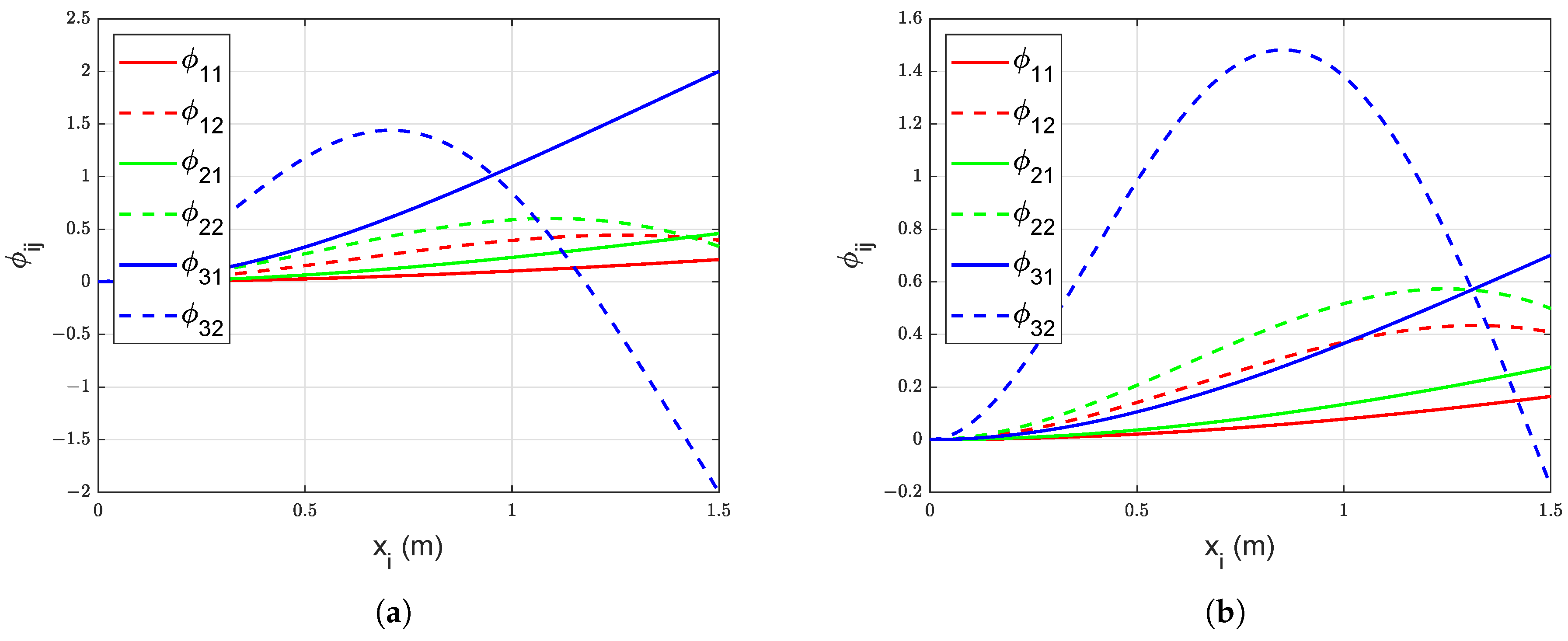
The effect of payload on the mode shapes and eigenfrequencies is studied with fixed robot configuration ($q_{r2}=0^{\circ }$ and $q_{r3}=0^{\circ }$). The mode shapes are calculated with the step of 0.01 m. The mode shapes under no payload ($m_p$ = 0 kg) and nominal payload ($m_p$ = 2 kg) conditions are shown in Figure 2a,b respectively. The effect of payload on the mode shapes of link 3 is more evident compared to its effect on the other two links. The eigenfrequencies for links 1, 2, and 3 under no payload and nominal payload conditions are tabulated in

Table 3. Effect of payload on eigenfrequencies.

	Eigenfrequencies (Hz) ${\mathit{f}}_{\mathit{i}}=\left[\begin{array}{cc}{\mathit{f}}_{\mathit{i}1}& {\mathit{f}}_{\mathit{i}2}\end{array}\right]$
	${\mathit{m}}_{\mathit{p}}$ = 0 kg	${\mathit{m}}_{\mathit{p}}$ = 2 kg
Link 1	$\left[\begin{array}{cc}2.56& 17.38\end{array}\right]$	$\left[\begin{array}{cc}2.02& 15.03\end{array}\right]$
Link 2	$\left[\begin{array}{cc}4.34& 28.74\end{array}\right]$	$\left[\begin{array}{cc}2.67& 18.82\end{array}\right]$
Link 3	$\left[\begin{array}{cc}14.17& 88.82\end{array}\right]$	$\left[\begin{array}{cc}4.90& 63.97\end{array}\right]$

. The results show that the eigenfrequencies decrease with the increase in payload.

4.2. Effect of Arm Configuration on Mode Shapes and Eigenfrequencies

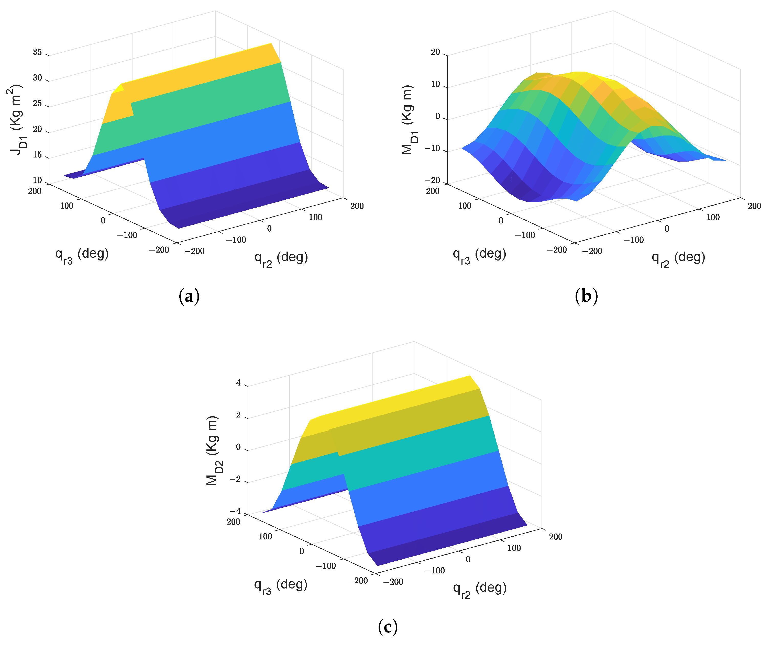
The effect of arm configuration on mode shapes and eigenfrequencies is studied by dividing the arm configuration ($q_{r1}$, $q_{r1}$, and $q_{r1}$) uniformly from $-{180}^{\circ }$ to ${180}^{\circ }$ with a step of ${30}^{\circ }$. It can be noticed (see Equations (69) and (71)) that the changes in the manipulator configuration, change the boundary values $J_{D1}$, $M_{D1}$, and $M_{D2}$, which are shown in Figure 3. This in turn modifies the mode shapes and eigenfrequencies of link 1 and link 2. To study the effect of change in manipulator configuration, the mode shapes and eigenfrequencies are calculated with nominal payload ($m_p$ = 2 kg) for different arm positions.

The change in $q_{r1}$ does not alter the mode shapes (and eigenfrequencies) of any of the links. The variation in mode shapes of link 1 with the change in $q_{r2}$ keeping $q_{r3}$ ($=0$) constant is shown in Figure 4a. Similarly, Figure 4b shows the change in mode shapes of link 1 with the change in $q_{r3}$ keeping $q_{r2}$($=0^{\circ }$) constant. For link 2, the change in $q_{r1}$ and $q_{r2}$ does not affect its mode shapes (and eigenfrequencies). The change in mode shapes of link 2 occurs with the change in $q_{r3}$ which is shown in Figure 4c. The mode shapes (and eigenfrequencies) of link 3 remain unaffected with any changes in manipulator configuration. The constant mode shapes of link 3 for all manipulator configurations with nominal payload are given in Figure 2b.

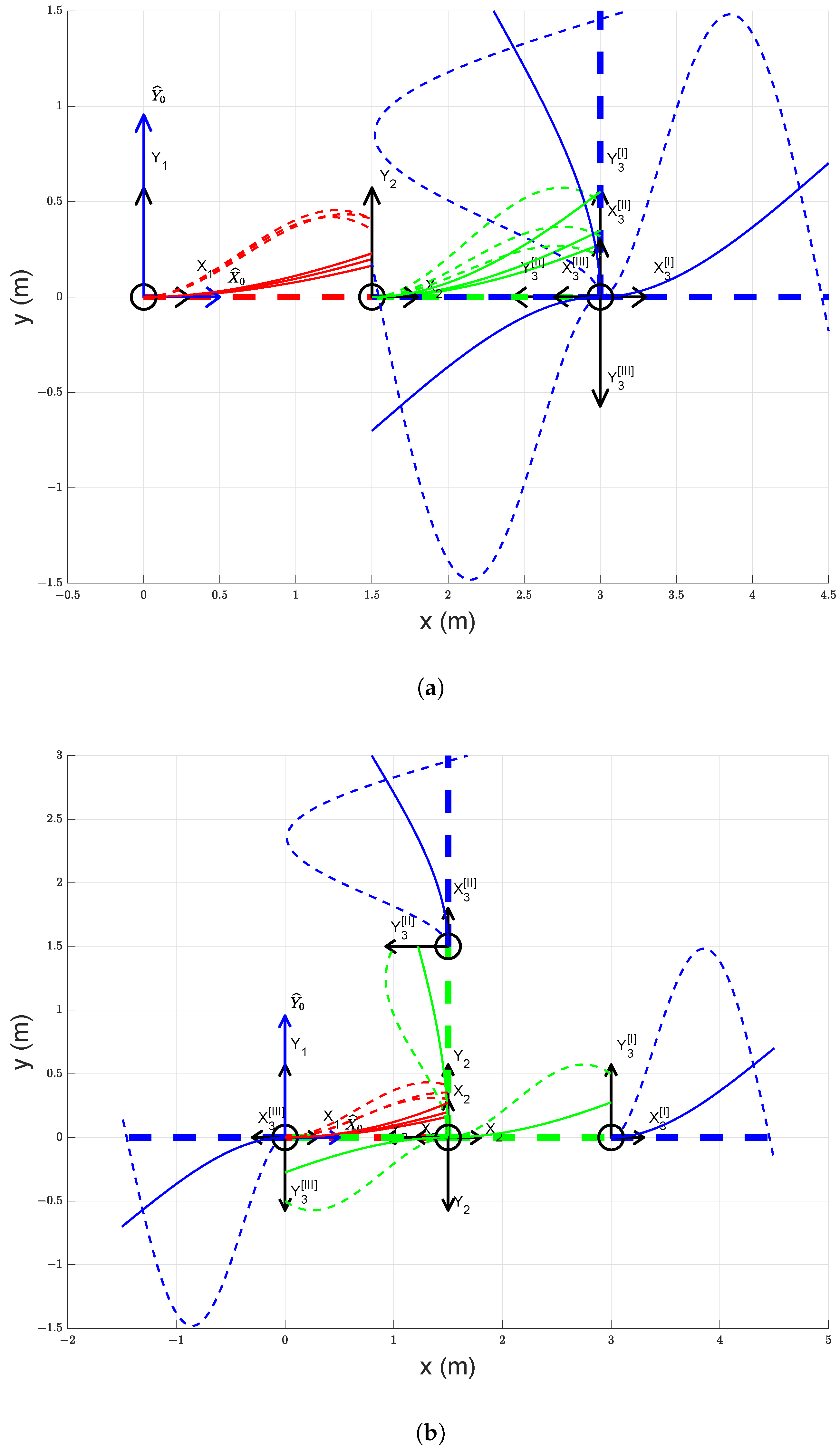
The overall effect of arm configuration on mode shapes is visualized in Figure 5, where only a few manipulator configurations are shown along with the corresponding mode shapes of each link. The links are represented by thick dashed lines (link 1: red, link 2: green, and link 3: blue), and the mode shapes are represented by thinner lines with a color corresponding to the links. The thinner solid lines represent mode shapes corresponding to the first modes and the thinner dashed lines represent the mode shapes corresponding to the second modes of the links. The joint coordinate frame ($X_i,Y_i$) of link i is represented by black arrowed lines, where the new positions of the frames are marked with [I], [II] and [III] for $0^{\circ }$, ${90}^{\circ }$, and ${180}^{\circ }$ rotations respectively.

In Figure 5a, link 3 is rotated about joint 3 (i.e., $q_{r3}$ is varied) by $0^{\circ }$ (I), ${90}^{\circ }$ (II), and ${180}^{\circ }$ (III) keeping $q_{r1}=0^{\circ }$ and $q_{r2}=0^{\circ }$ constant. It is observable that the mode shapes of both links 1 and 2 changed with the change in $q_{r3}$. In Figure 5b, link 2 is rotated about joint 2 (i.e., $q_{r2}$ is varied) by $0^{\circ }$ (I), ${90}^{\circ }$ (II), and ${180}^{\circ }$ (III) keeping $q_{r1}=0^{\circ }$ and $q_{r3}=0^{\circ }$ constant. It can be noticed that the mode shapes of link 1 alter with the change in $q_{r3}$ but that of links 2 and 3 remain unaltered.

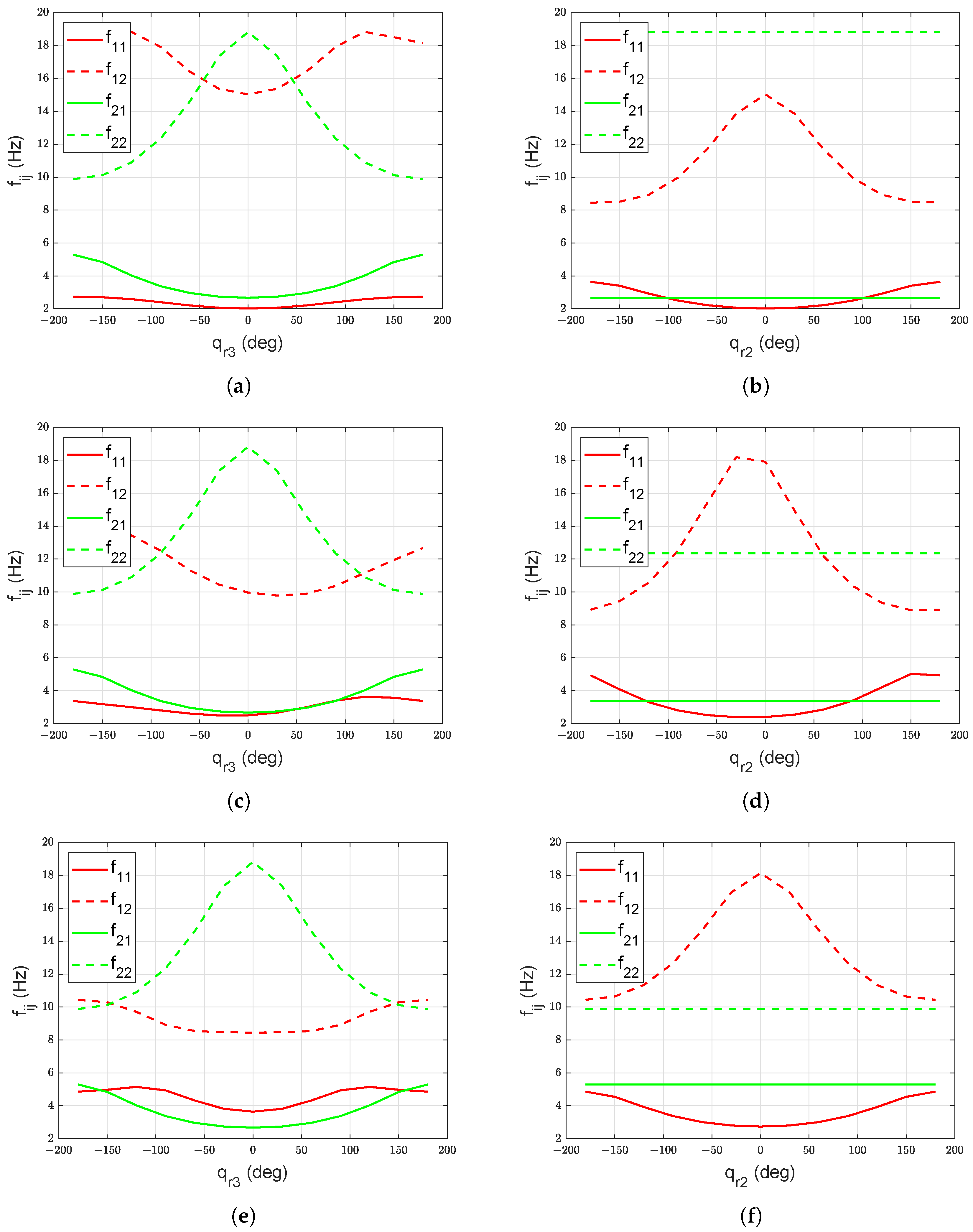
The effect of $q_{r3}$ on the eigenfrequencies of link 1 and link 2 is shown in Figure 6a,c,e, with the constant $q_{r2}$ at $0^{\circ }$, ${90}^{\circ }$, and ${180}^{\circ }$ respectively. Similarly, the effect of $q_{r2}$ on the eigenfrequencies of link 1 and link 2 is shown in Figure 6b,d,f, with the constant $q_{r3}$ at $0^{\circ }$, ${90}^{\circ }$, and ${180}^{\circ }$ respectively. The eigenfrequencies of link 2 remains unchanged with the change in $q_{r1}$ and $q_{r2}$. The eigenfrequencies of link 3 remain unaffected by any change in $q_{r1}$, $q_{r2}$, and $q_{r3}$. The constant eigenfrequencies of link 3 for all manipulator configurations with nominal payload are given in Table 3. Similarly, the eigenfrequencies of link 1, link 2, and link 3 are not altered by any variation in $q_{r1}$.

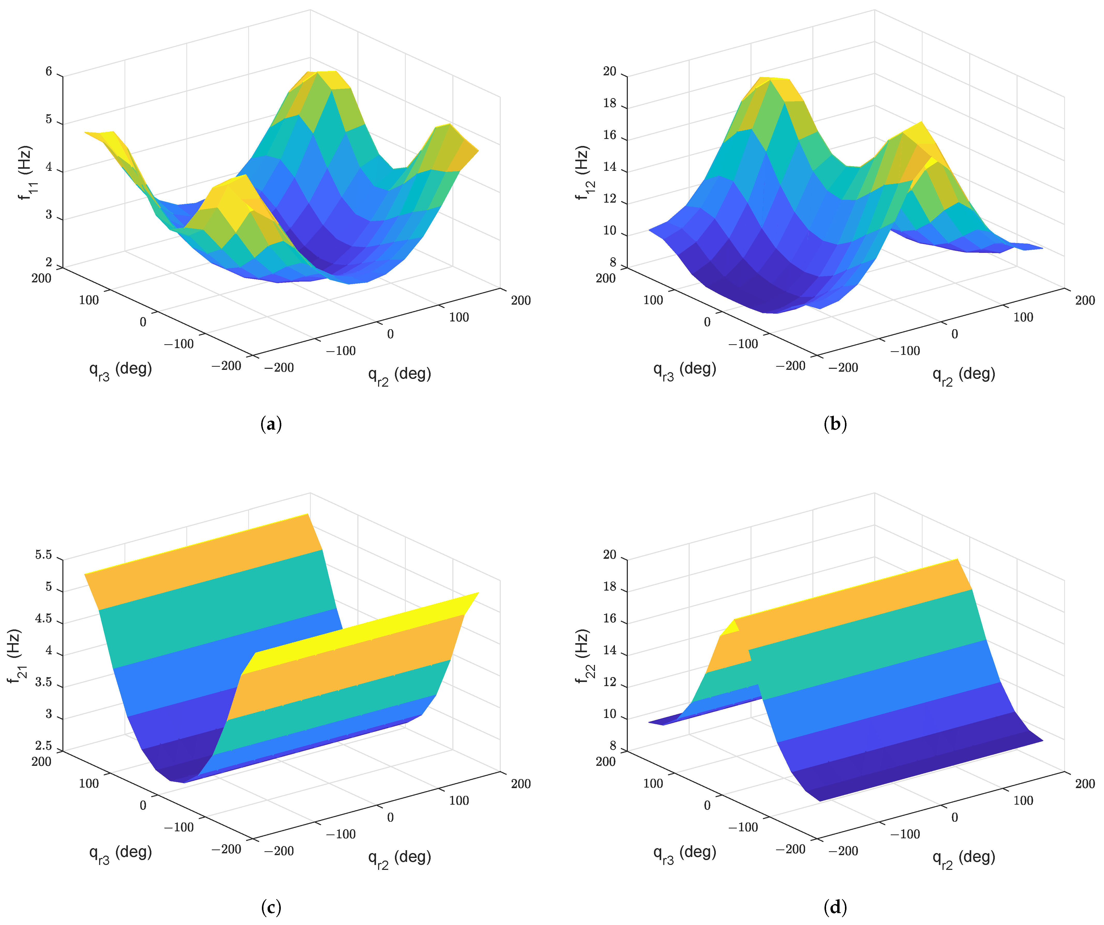
The overall effect of arm configuration on the eigenfrequencies of link 1 and link 2 is shown in Figure 7.

4.3. Time-Domain Simulation

A set of numerical simulations have been performed to validate the theoretical model. The equations of motion are integrated using a fourth-order Runge-Kutta method with a fixed step size of 1 ms. The free and forced vibration responses of the dynamic model have been simulated. The nominal payload ($m_p$ = 2 kg) condition is used for all time-domain simulations.

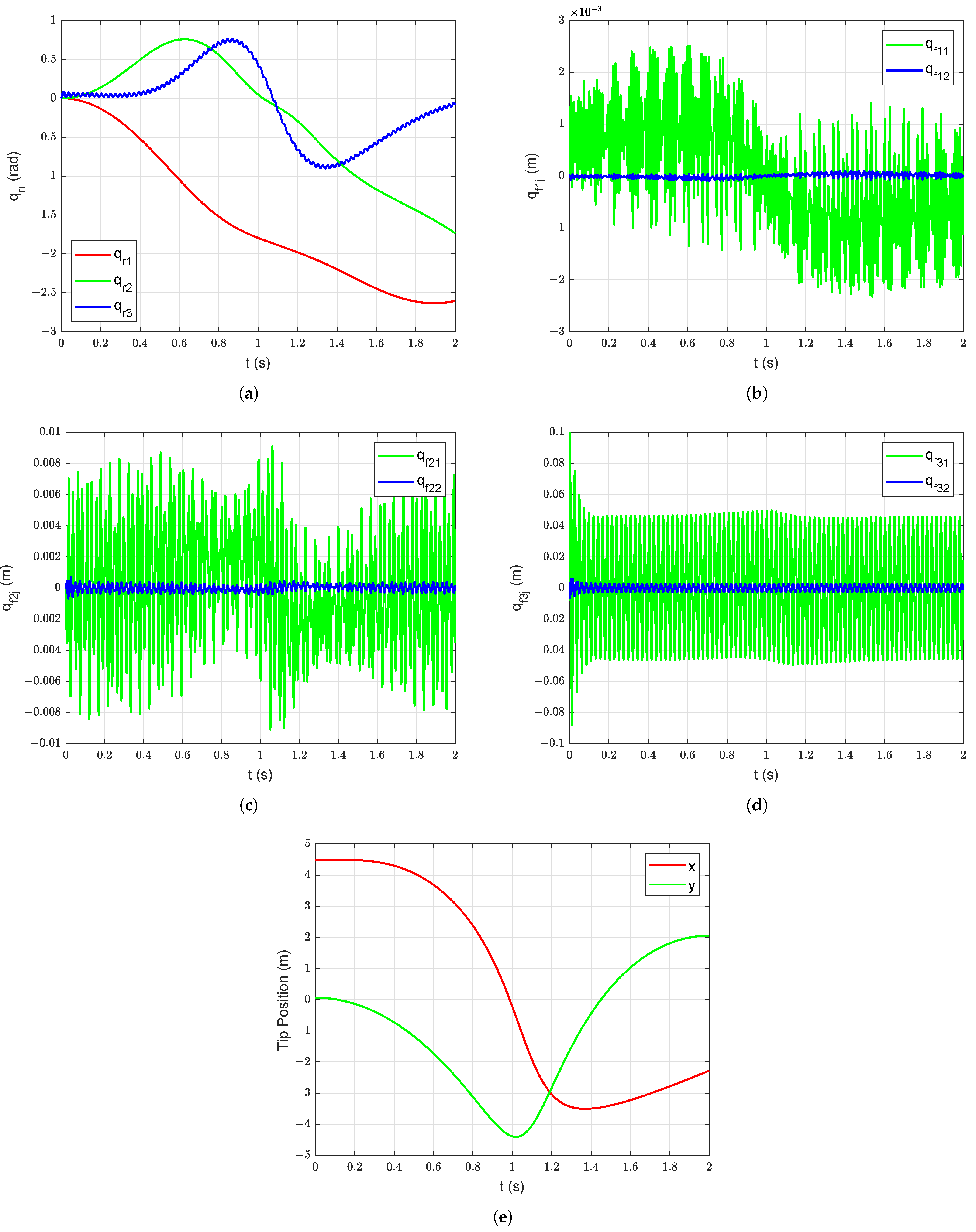
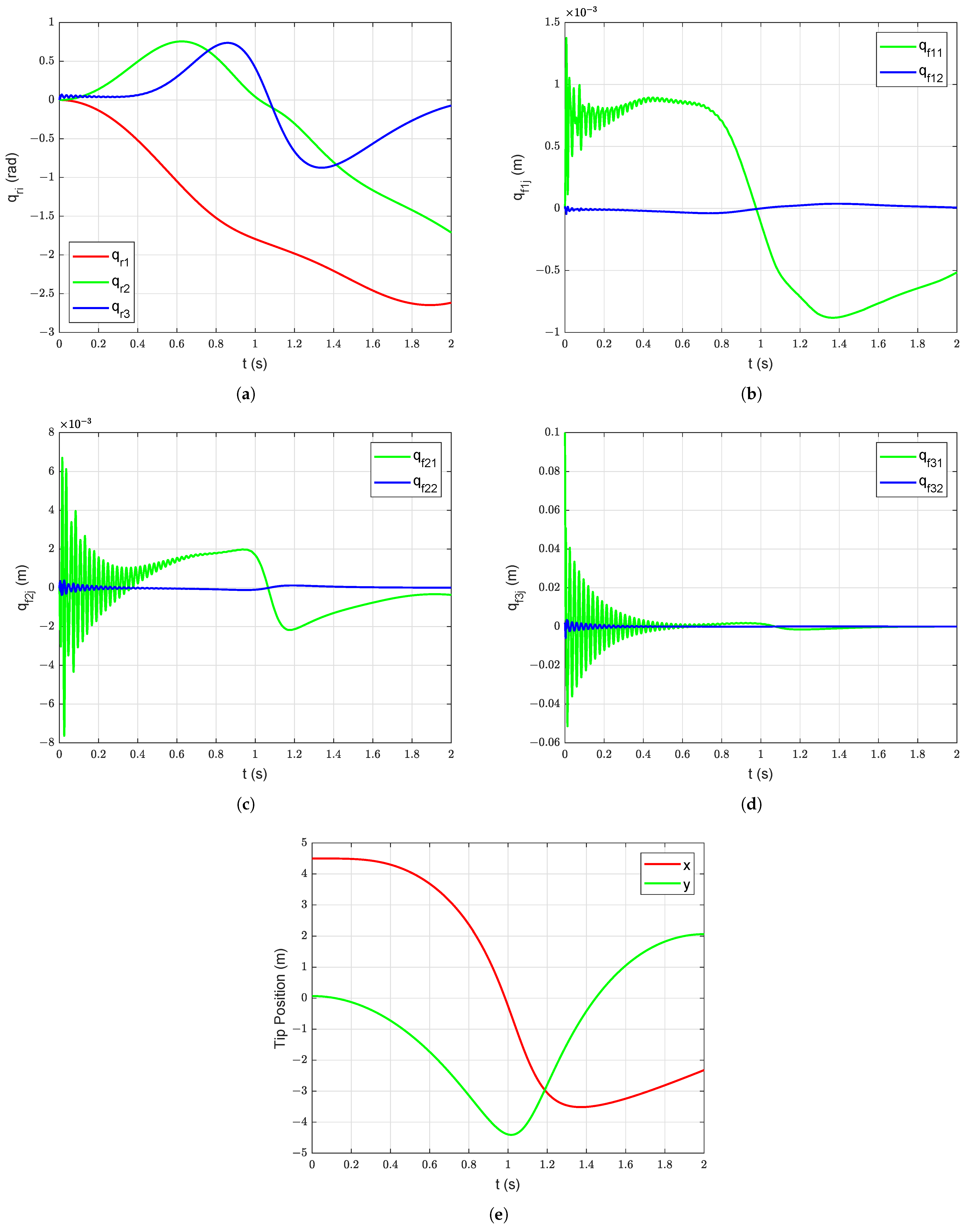
Firstly, free vibration response of the system is simulated without structural (and viscus) damping under gravity starting with initial deformation in link 3 ($q_{r1}\left(0\right)$ = $q_{r2}\left(0\right)$ = $q_{r3}\left(0\right)$ = $0^{\circ }$, $q_{f11}\left(0\right)$ = $q_{f12}\left(0\right)$ = $q_{f21}\left(0\right)$ = $q_{f22}\left(0\right)$ = 0 m, $q_{f31}\left(0\right)$ = 0.1 m, and $q_{f32}\left(0\right)$ = 0.002 m). The associated joint positions, link deflections, and tip motion are shown in Figure 8. Then, the passive structural damping (${\zeta }_{11}$ = ${\zeta }_{12}$ = ${\zeta }_{21}$ = ${\zeta }_{22}$ = ${\zeta }_{31}$ = ${\zeta }_{32}$ = $0.005$, $b_1$ = $b_2$ = $b_3$ = 0) is added into the system. The free vibration response of the system with passive structural damping under gravity starting with initial deformation ($q_{f31}\left(0\right)$ = 0.1 m and $q_{f32}\left(0\right)$ = 0.002 m) is shown in Figure 9. The benefits of adding passive structural damping are evident from Figure 8 and Figure 9. The overall manipulator motion is improved because of the addition of the passive damping in the arm structure.

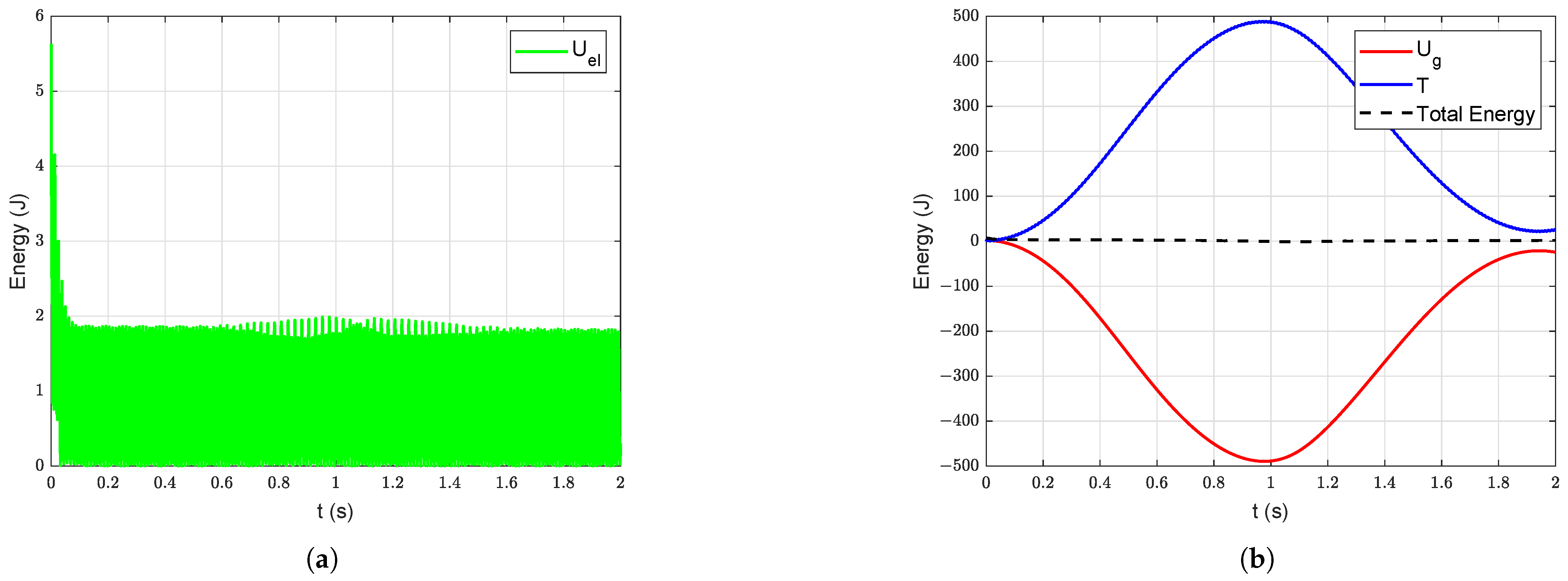
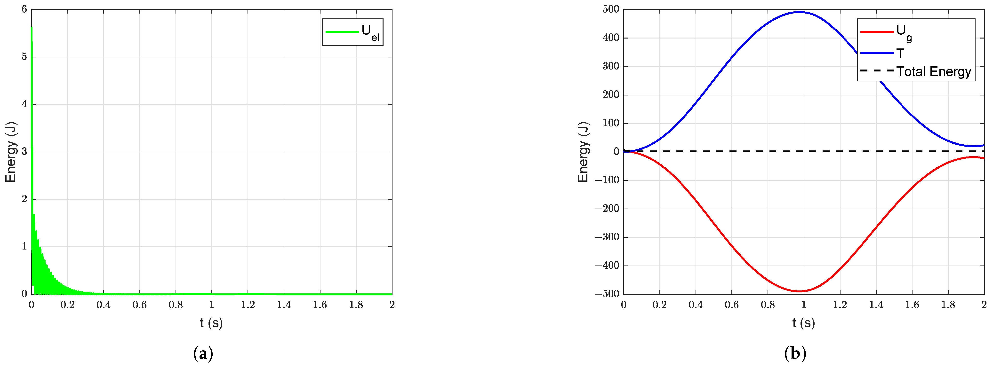
For empirical validation of the model, energies of the system under free vibration are considered. The elastic potential energy ($U_{el}$) of the system without damping is shown in Figure 10a. Similarly, the potential energy due to gravity ($U_g$), kinetic energy (T) and the total mechanical energy of the system without damping are shown in Figure 10b. The corresponding energies of the system when the damping is introduced into the system are shown in Figure 11. In Figure 11a, the elastic energy is high in the beginning (because of the initial deformation ($q_{f31}\left(0\right)$ = 0.1 m and $q_{f32}\left(0\right)$ = 0.002 m) introduced into the system) and it gradually decreases due to structural damping. It is evident from Figure 11a,b that the total energy of the system is decreasing due to damping.

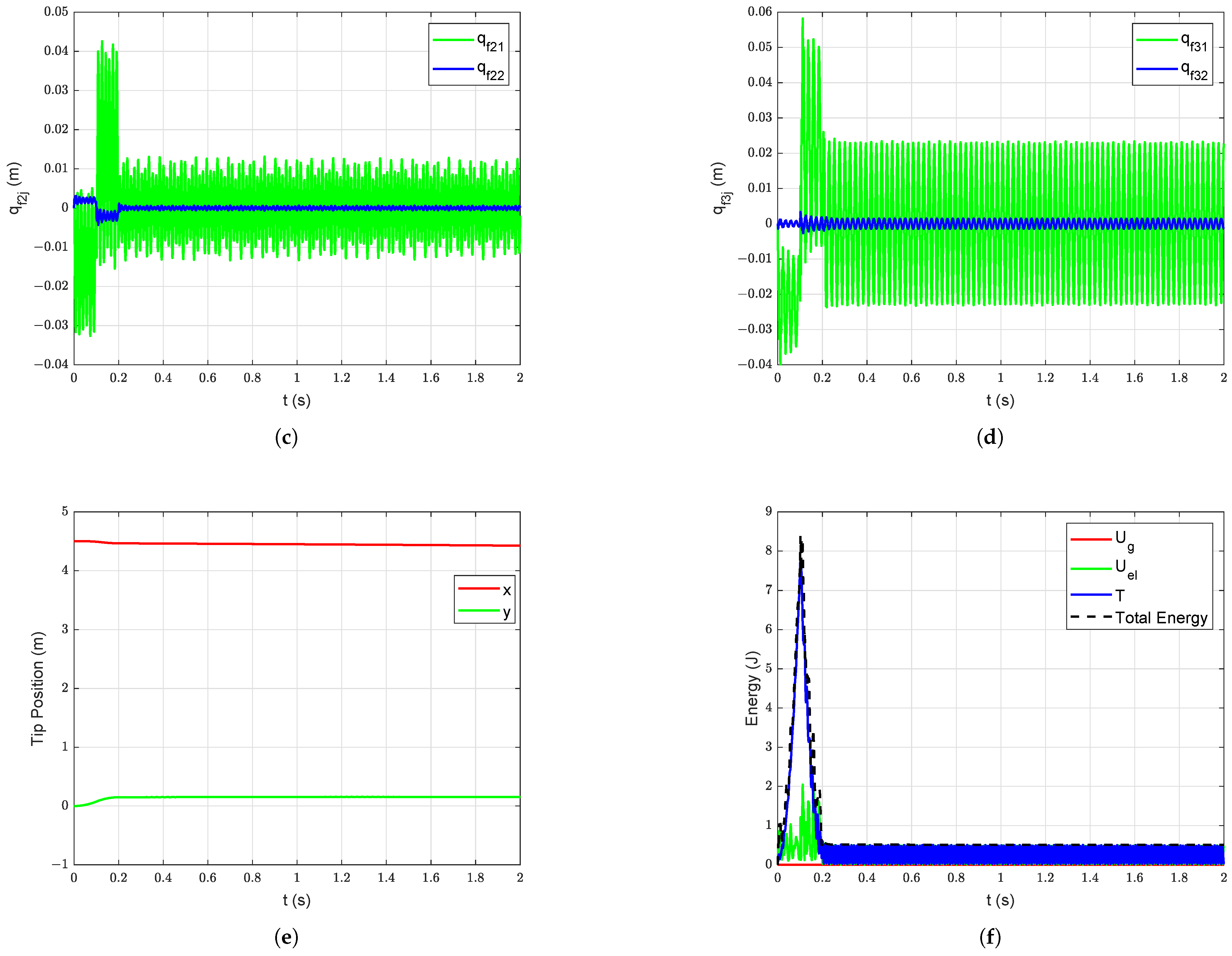
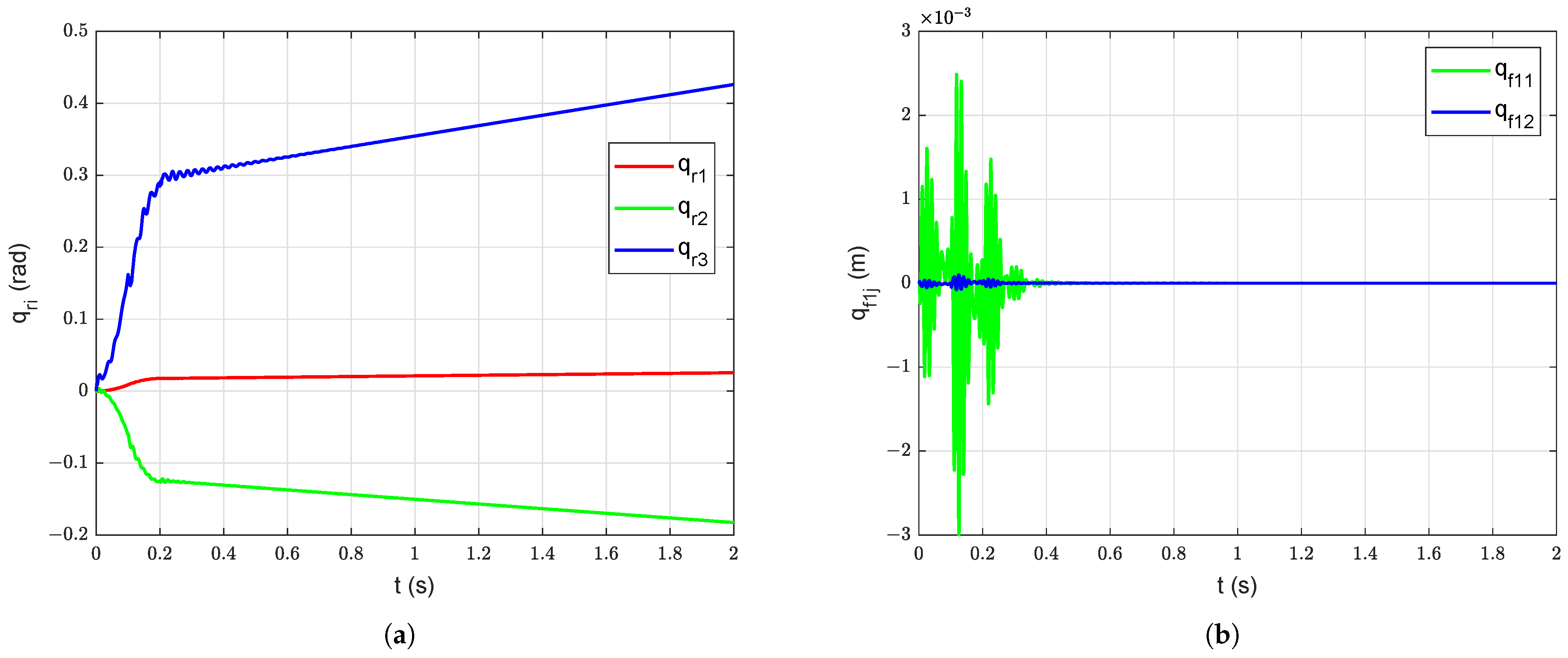
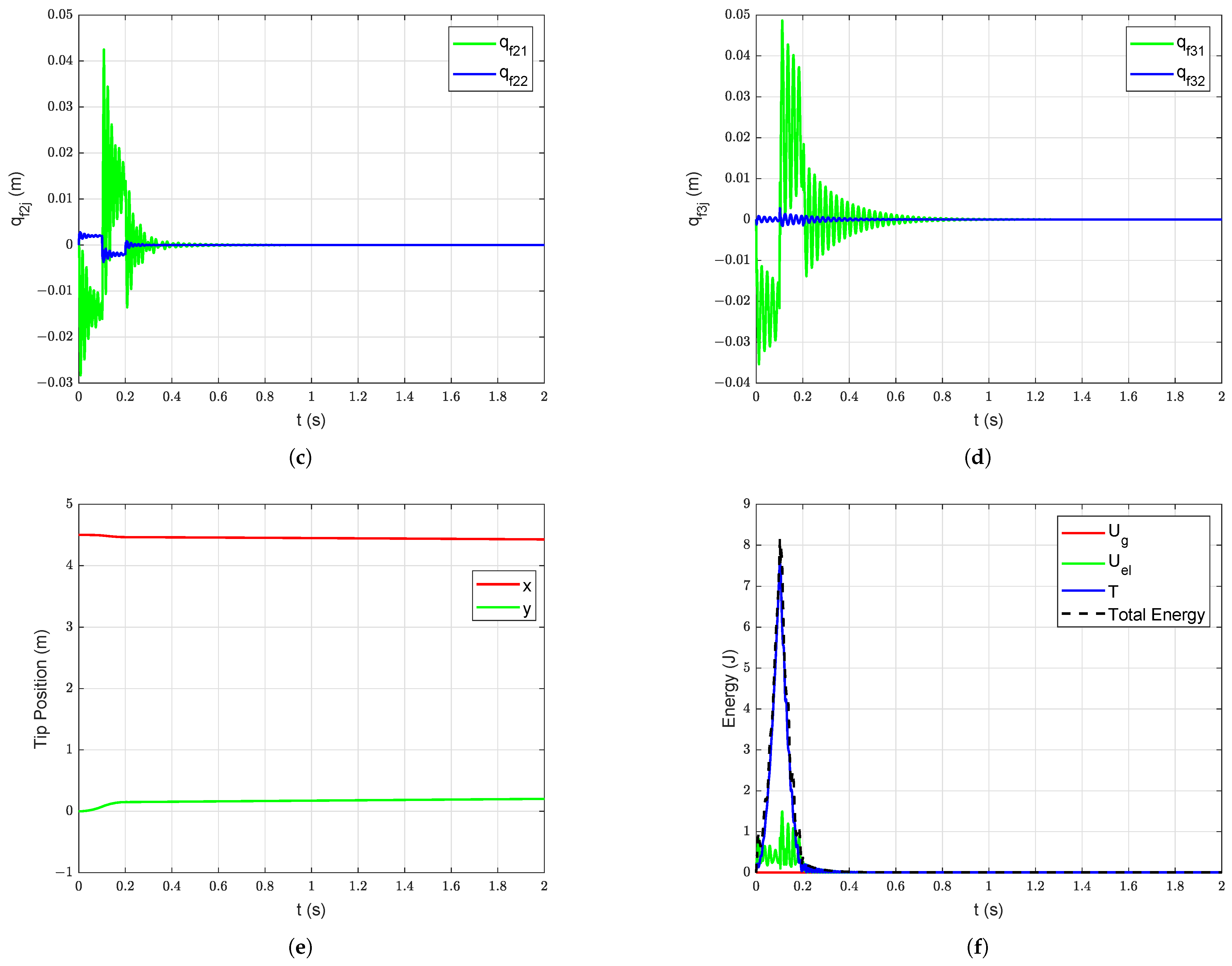
The forced vibration response of the system is studied by applying a symmetric bang-bang input torque with an amplitude of 50 Nm and acceleration (and deceleration) period of 0.1 s at joint 3 starting from $q_{r1}\left(0\right)$ = $q_{r2}\left(0\right)$ = $q_{r3}\left(0\right)$ = $0^{\circ }$, and $q_{f11}\left(0\right)$ = $q_{f12}\left(0\right)$ = $q_{f21}\left(0\right)$ = $q_{f22}\left(0\right)$ = $q_{f31}\left(0\right)$ = $q_{f32}\left(0\right)$ = 0 m (undeformed configuration). The effect of gravity is ignored in this study (i.e., ${\mathit{g}}_v = \left[\begin{array}{cc}0& 0\end{array}\right]$${}^T$ ms${}^{-2}$) to show the coupled vibrations induced only due to bang-bang input torque. The forced vibration of all links at the joints and the tip level without damping are shown in Figure 12. The forced vibration response of the system after the passive structural damping (${\zeta }_{11}$ = ${\zeta }_{12}$ = ${\zeta }_{21}$ = ${\zeta }_{22}$ = ${\zeta }_{31}$ = ${\zeta }_{32}$ = $0.005$, $b_1$ = $b_2$ = $b_3$ = 0) is introduced into the system without gravity starting with undeformed configuration is shown in Figure 13. The slow relative drifting phenomenon is observable in the joint trajectories shown in Figure 12a,b [6]. The coupled vibrations induced in all links are smoothed down with the introduction of damping. The potential energy due to gravity ($U_g=0$), elastic potential energy ($U_{el}$), kinetic energy (T) and the total mechanical energy of the system without damping are shown in Figure 12f and corresponding energies with damping are shown in Figure 13f.

4.4. Frequency-Domain Analysis

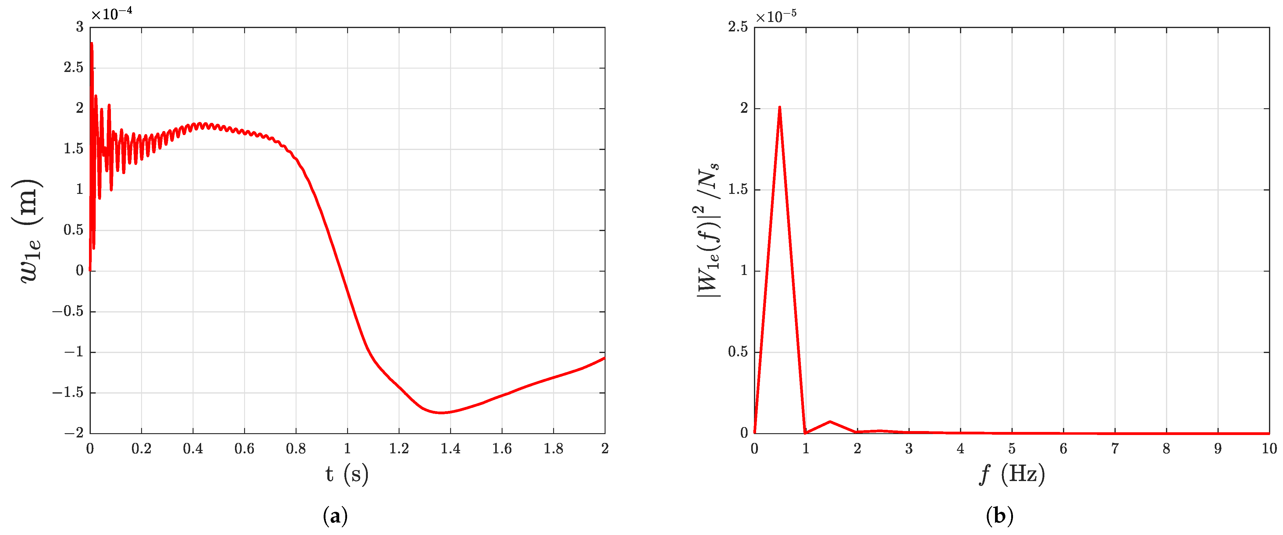
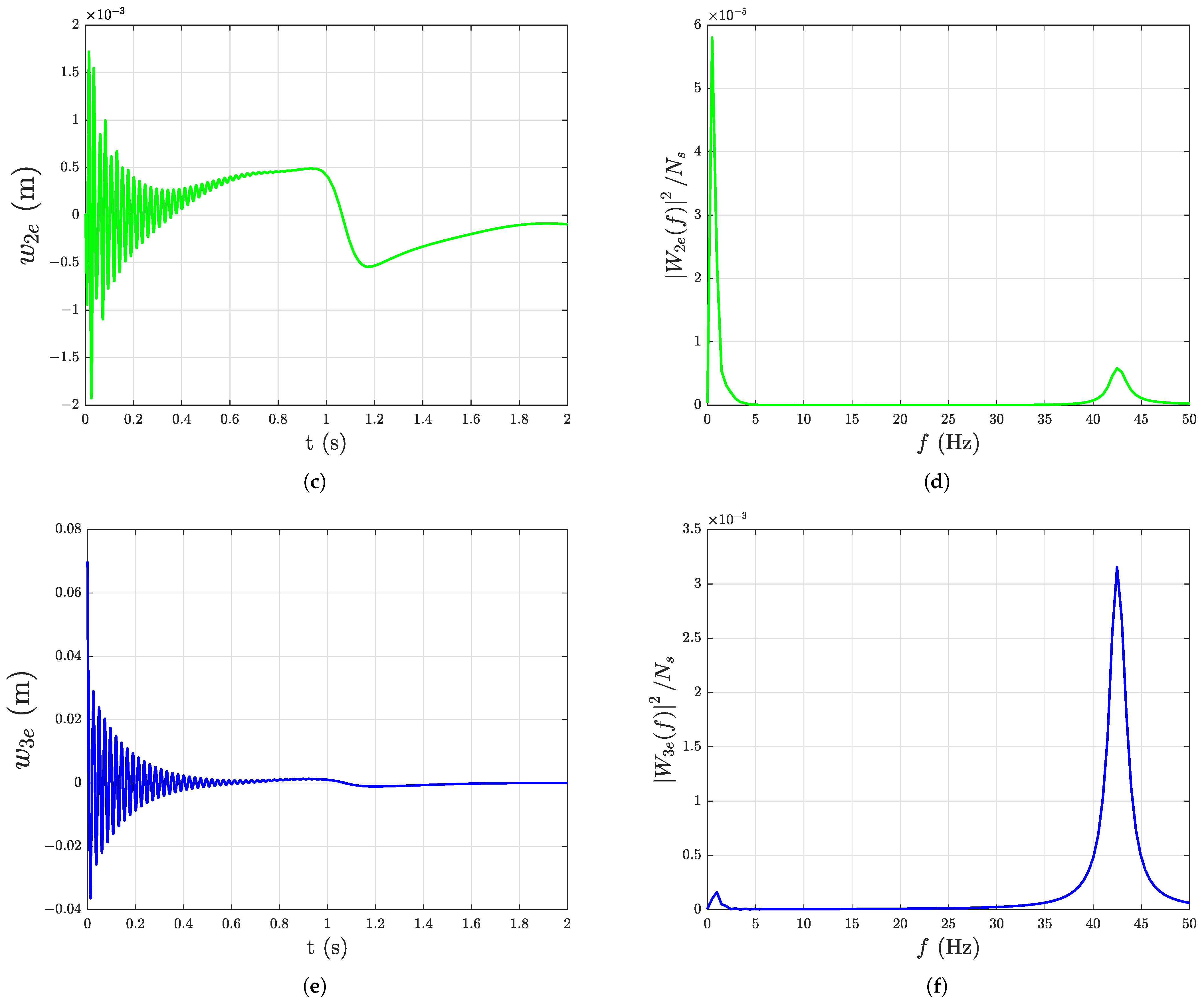
The deflection of the tip of each link $w_{ie}={\left.w_i\right|}_{x_i={\ell }_i}$ of the manipulator with damping under gravity starting with initial deformation in link 3 ($q_{r1}\left(0\right)=q_{r2}\left(0\right)=q_{r3}\left(0\right)=0^{\circ }$, $q_{f11}\left(0\right)=q_{f12}\left(0\right)=q_{f21}\left(0\right)=q_{f22}\left(0\right)$ = 0 m, $q_{f31}\left(0\right)$ = 0.1 m, and $q_{f32}\left(0\right)$ = 0.002 m) is considered for the frequency-domain analysis. The nominal payload is used and the deflection values are recorded for $2s$ with a fixed step size of $1ms$ for this study.

A fast Fourier transform algorithm is used to compute the Fourier transform of the deflection signal which contains $N_s=2000$ number of samples. The power spectrum of the discrete Fourier transform $W_{ie}\left(f\right)$ of the deflection $w_{ie}$ of link i is computed for all links using the uniformly sampled (at $1ms$) time-domain deflection signal of the tip of each link. The deflection of the tip of each link and its corresponding frequency response (power spectrum) is shown in Figure 14a–f, where $\left|W_{ie}\left(f\right)\right|$ is the amplitude of the discrete Fourier transform of $w_{ie}$ corresponding to link i and f is the frequency of the signal in Hz. From Figure 14a–f, the frequency components of the deflection signal of each link are revealed by the spikes in the power as follows: Link 1: 0.4883 Hz, 1.465 Hz; Link 2: 0.883 Hz, 42.48 Hz; and Link 3: 0.9766 Hz, 42.48 Hz.

5. Conclusions and Discussions

The closed-form dynamic model of the planar multi-link flexible manipulator is derived and the results of the time-domain and frequency-domain simulation of a three-link manipulator are reported. The effect of robot configuration and payload on the mode shapes and eigenfrequencies of the flexible links are discussed.

The mathematical model of the planar three-link flexible manipulator developed in this work will be experimentally validated in the future. The dynamic model developed in this work will be used for developing and testing (model-based) controllers and for simulation-based trajectory optimization.

References

- Subedi, D.; Tyapin, I.; Hovland, G. Review on Modeling and Control of Flexible Link Manipulators. Model. Identif. Control 2020, 41, 141–163. [Google Scholar] [CrossRef]
- Theodore, R.J.; Ghosal, A. Comparison of the Assumed Modes and Finite Element Models for Flexible Multilink Manipulators. Int. J. Robot. Res. 1995, 14, 91–111. [Google Scholar] [CrossRef] [Green Version]
- Krauss, R. An Improved Approach for Spatial Discretization of Transfer Matrix Models of Flexible Structures. In Proceedings of the 2019 American Control Conference (ACC), Philadelphia, PA, USA, 10–12 July 2019; pp. 3123–3128. [Google Scholar] [CrossRef]
- Tokhi, M.O.; Azad, A.K.M. Flexible Robot Manipulators: Modelling, Simulation and Control; IET: London, UK, 2008; Volume 68. [Google Scholar]
- De Luca, A.; Lanari, L.; Lucibello, P.; Panzieri, S.; Ulivi, G. Control experiments on a two-link robot with a flexible forearm. In Proceedings of the 29th IEEE Conference on Decision and Control, Honolulu, HI, USA, 5–7 December 1990; Volume 2, pp. 520–527. [Google Scholar] [CrossRef]
- Luca, A.D.; Siciliano, B. Closed-Form Dynamic Model of Planar Multilink Lightweight Robots. IEEE Trans. Syst. Man Cybern. 1991, 21, 826–839. [Google Scholar] [CrossRef]
- Vera, F.G.D. Modeling and Sliding-Mode Control of Flexible-Link Robotic Structures for Vibration Suppression; Technische Universität Clausthal: Clausthal-Zellerfeld, Germany, 2016. [Google Scholar]
- Zhang, X.; Mills, J.K.; Cleghorn, W.L. Dynamic Modeling and Experimental Validation of a 3-PRR Parallel Manipulator with Flexible Intermediate Links. J. Intell. Robot. Syst. 2007, 50, 323–340. [Google Scholar] [CrossRef]
- Book, W.J. Modeling, design, and control of flexible manipulator arms: A tutorial review. In Proceedings of the 29th IEEE Conference on Decision and Control, Honolulu, HI, USA, 5–7 December 1990; Volume 2, pp. 500–506. [Google Scholar] [CrossRef]
- Kurfess, T.R. Robotics and Automation Handbook; CRC Press: Boca Raton, FL, USA, 2018. [Google Scholar]
- Rahimi, H.N.; Nazemizadeh, M. Dynamic analysis and intelligent control techniques for flexible manipulators: A review. Adv. Robot. 2014, 28, 63–76. [Google Scholar] [CrossRef]
- Lochan, K.; Roy, B.K.; Subudhi, B. A review on two-link flexible manipulators. Annu. Rev. Control 2016, 42, 346–367. [Google Scholar] [CrossRef]
- Koutsovasilis, P.; Beitelschmidt, M. Comparison of model reduction techniques for large mechanical systems. Multibody Syst. Dyn. 2008, 20, 111–128. [Google Scholar] [CrossRef]
- Vidoni, R.; Scalera, L.; Gasparetto, A.; Giovagnoni, M. Comparison of model order reduction techniques for flexible multibody dynamics using an equivalent rigid-link system approach. In Proceedings of the 8th ECCOMAS Thematic Conference on Multibody Dynamics, Prague, Czech Republic, 19–22 June 2017; pp. 269–280. [Google Scholar]
- Wu, L.; Tiso, P.; van Keulen, F. A modal derivatives enhanced Craig-Bampton method for geometrically nonlinear structural dynamics. In Proceedings of the ISMA, Leuven, Belgium, 19–21 September 2016; pp. 3615–3624. [Google Scholar]
- Tang, L.; Gouttefarde, M.; Sun, H.; Yin, L.; Zhou, C. Dynamic modelling and vibration suppression of a single-link flexible manipulator with two cables. Mech. Mach. Theory 2021, 162, 104347. [Google Scholar] [CrossRef]
- Vidoni, R.; Scalera, L.; Gasparetto, A. 3-D ERLS based dynamic formulation for flexible-link robots: Theoretical and numerical comparison between the finite element method and the component mode synthesis approaches. Int. J. Mech. Control 2018, 19, 39–50. [Google Scholar]
- Korayem, M.H.; Dehkordi, S.F. Dynamic modeling of flexible cooperative mobile manipulator with revolute-prismatic joints for the purpose of moving common object with closed kinematic chain using the recursive Gibbs-Appell formulation. Mech. Mach. Theory 2019, 137, 254–279. [Google Scholar] [CrossRef]
- Zhang, C.; Yang, T.; Sun, N.; Zhang, J. A Simple Control Method of Single-Link Flexible Manipulators. In Proceedings of the 3rd International Symposium on Autonomous Systems, ISAS 2019, Shanghai, China, 29–31 May 2019; pp. 300–304. [Google Scholar] [CrossRef]
- Liu, Z.; Liu, J.; He, W. Dynamic modeling and vibration control for a nonlinear 3-dimensional flexible manipulator. Int. J. Robust Nonlinear Control 2018, 28, 3927–3945. [Google Scholar] [CrossRef]
- Meng, Q.X.; Lai, X.Z.; Wang, Y.W.; Wu, M. A fast stable control strategy based on system energy for a planar single-link flexible manipulator. Nonlinear Dyn. 2018, 94, 615–626. [Google Scholar] [CrossRef]
- He, W.; He, X.; Zou, M.; Li, H. PDE Model-Based Boundary Control Design for a Flexible Robotic Manipulator with Input Backlash. IEEE Trans. Control Syst. Technol. 2018, 27, 790–797. [Google Scholar] [CrossRef]
- Sun, C.; Gao, H.; He, W.; Yu, Y. Fuzzy Neural Network Control of a Flexible Robotic Manipulator Using Assumed Mode Method. IEEE Trans. Neural Netw. Learn. Syst. 2018, 29, 5214–5227. [Google Scholar] [CrossRef] [PubMed]
- Reddy, M.P.P.; Jacob, J. Vibration control of flexible link manipulator using SDRE controller and Kalman filtering. Stud. Inform. Control 2017, 26, 143–150. [Google Scholar] [CrossRef] [Green Version]
- Ghasemi, A.H. Slewing and vibration control of a single-link flexible manipulator using filtered feedback linearization. J. Intell. Mater. Syst. Struct. 2017, 28, 2887–2895. [Google Scholar] [CrossRef]
- Ouyang, Y.; He, W.; Li, X.; Liu, J.K.; Li, G. Vibration Control Based on Reinforcement Learning for a Single-link Flexible Robotic Manipulator. IFAC-PapersOnLine 2017, 50, 3476–3481. [Google Scholar] [CrossRef]
- Ouyang, Y.; He, W.; Li, X. Reinforcement learning control of a singlelink flexible robotic manipulator. IET Control Theory Appl. 2017, 11, 1426–1433. [Google Scholar] [CrossRef]
- Lochan, K.; Roy, B.K. Second-order SMC for tip trajectory tracking and tip deflection suppression of an AMM modelled nonlinear TLFM. Int. J. Dyn. Control 2018, 6, 1310–1318. [Google Scholar] [CrossRef]
- Singla, A.; Singh, A. Dynamic Modeling of Flexible Robotic Manipulators. In Harmony Search and Nature Inspired Optimization Algorithms; Yadav, N., Yadav, A., Bansal, J.C., Deep, K., Kim, J.H., Eds.; Springer Singapore: Singapore, 2019; pp. 819–834. [Google Scholar]
- Qiu, Z.c.; Li, C.; min Zhang, X. Experimental study on active vibration control for a kind of two-link flexible manipulator. Mech. Syst. Signal Process. 2019, 118, 623–644. [Google Scholar] [CrossRef]
- Gao, H.; He, W.; Zhou, C.; Sun, C. Neural Network Control of a Two-Link Flexible Robotic Manipulator Using Assumed Mode Method. IEEE Trans. Ind. Inform. 2018, 15, 755–765. [Google Scholar] [CrossRef]
- Pradhan, S.K.; Subudhi, B. Position control of a flexible manipulator using a new nonlinear self-Tuning PID controller. IEEE/CAA J. Autom. Sin. 2020, 7, 136–149. [Google Scholar] [CrossRef]
- Giorgio, I.; Del Vescovo, D.D. Non-linear lumped-parameter modeling of planar multi-link manipulators with highly flexible arms. Robotics 2018, 7, 60. [Google Scholar] [CrossRef] [Green Version]
- Subedi, D.; Tyapin, I.; Hovland, G. Modeling and Analysis of Flexible Bodies Using Lumped Parameter Method. In Proceedings of the 2020 IEEE 11th International Conference on Mechanical and Intelligent Manufacturing Technologies (ICMIMT), Cape town, South Africa, 20–22 January 2020; pp. 161–166. [Google Scholar] [CrossRef]
Figure 1.
Planar three-link flexible manipulator.
Figure 2.
(a) Mode shapes for link 1, 2, and 3 with no payload ( = 0 kg), , and , (b) Mode shapes for link 1, 2, and 3 with nominal payload ( = 2 kg), , and .
Figure 3.
(a) with nominal payload, (b) with nominal payload, (c) with nominal payload.
Figure 4.
(a) Mode shapes for link 1 with nominal payload and , (b) Mode shapes for link 1 with nominal payload and , (c) Mode shapes for link 2 with nominal payload.
Figure 5.
(a) Mode shapes for link 1 (red), 2 (green), and 3 (blue) with nominal payload, , , and (I), (II), (III) (b) Mode shapes for link 1 (red), 2 (green), and 3 (blue) with nominal payload, , , and (I), (II), (III).
Figure 6.
(a) Eigenfrequencies for link 1 and 2 with nominal payload and , (b) Eigenfrequencies for link 1 and 2 with nominal payload and , (c) Eigenfrequencies for link 1 and 2 with nominal payload and , (d) Eigenfrequencies for link 1 and 2 with nominal payload and , (e) Eigenfrequencies for link 1 and 2 with nominal payload and , (f) Eigenfrequencies for link 1 and 2 with nominal payload and .
Figure 7.
(a) Eigenfrequency for link 1 with nominal payload, (b) Eigenfrequency for link 1 with nominal payload, (c) Eigenfrequency for link 2 with nominal payload, (d) Eigenfrequencies for link 2 with nominal payload.
Figure 8.
Free vibration response without damping under gravity starting with initial deformation ( = 0.1 m and = 0.002 m): (a) Joint Position, (b) Deflections of link 1, (c) Deflections of link 2, (d) Deflections of link 3, (e) Manipulator tip position.
Figure 9.
Free vibration response with damping under gravity starting with initial deformation ( = 0.1 m and = 0.002 m): (a) Joint Position, (b) Deflections of link 1, (c) Deflections of link 2, (d) Deflections of link 3, (e) Manipulator tip position.
Figure 10.
Energy of the manipulator system under free vibration without damping under gravity starting with initial deformation ( = 0.1 m and = 0.002 m): (a) Elastic energy, (b) Potential energy due to gravity, kinetic and total energy.
Figure 11.
Energy of the manipulator system under free vibration with damping under gravity starting with initial deformation ( = 0.1 m and = 0.002 m): (a) Elastic energy, (b) Potential energy due to gravity, kinetic and total energy.
Figure 12.
Forced vibration response without damping without gravity starting with undeformed configuration: (a) Joint Position, (b) Deflections of link 1, (c) Deflections of link 2, (d) Deflections of link 3, (e) Manipulator tip position, (f) Energy of the manipulator system.
Figure 13.
Forced vibration response with damping without gravity starting with undeformed configuration: (a) Joint Position, (b) Deflections of link 1, (c) Deflections of link 2, (d) Deflections of link 3, (e) Manipulator tip position, (f) Energy of the manipulator system.
Figure 14.
Time-domain and frequency-domain representation of tip deflection of the links with damping under gravity starting with initial deformation ( = 0.1 m and = 0.002 m): (a) Tip deflection of link 1, (b) Frequency response of the tip deflection of link 1, (c) Tip deflection of link 2, (d) Frequency response of the tip deflection of link 2, (e) Tip deflection of link 3, (f) Frequency response of the tip deflection of link 3.