
Mechatronic Model of a Compliant 3PRS Parallel Manipulator


Department of Mechanical Engineering, Faculty of Engineering, University of the Basque Country UPV/EHU, Plaza Ingeniero Torres Quevedo, 48013 Bilbao, Spain
*
Author to whom correspondence should be addressed.
Robotics 2022, 11(1), 4; https://0-doi-org.brum.beds.ac.uk/10.3390/robotics11010004
Submission received: 15 November 2021
/
Revised: 20 December 2021
/
Accepted: 21 December 2021
/
Published: 28 December 2021
(This article belongs to the Special Issue 10th Anniversary of Robotics—Feature Papers in Intelligent Robots and Mechatronics)
Abstract
:Compliant mechanisms are widely used for instrumentation and measuring devices for their precision and high bandwidth. In this paper, the mechatronic model of a compliant 3PRS parallel manipulator is developed, integrating the inverse and direct kinematics, the inverse dynamic problem of the manipulator and the dynamics of the actuators and the control. The kinematic problem is solved, assuming a pseudo-rigid model for the deflection in the compliant revolute and spherical joints. The inverse dynamic problem is solved, using the Principle of Energy Equivalence. The mechatronic model allows the prediction of the bandwidth of the manipulator motion in the 3 degrees of freedom for a given control and set of actuators, helping in the design of the optimum solution. A prototype is built and validated, comparing experimental signals with the ones from the model.
1. Introduction
The use of compliance in mechanisms has become very common for several purposes. Compliant and continuum mechanisms make use of the flexibility of some parts of the mechanism to achieve motion with several degrees of freedom. While continuum mechanisms present slender elements that deflect along their whole length, compliant mechanism are composed of rigid elements joined by flexure hinges that deform under the application of a load [1,2]. Other applications of compliance can be found in the interaction with human or other elements, where a variable stiffness must be provided by the actuators to resemble a physiological response [3,4,5].
Among those applications of compliance, compliant mechanisms have found a place in applications that require short range of motion, high precision, high bandwidth, special environmental conditions, such as high vacuum, and one or more degrees of freedom. In [6], a mechanism for a single-axis nano-positioning stage is presented with a range of motion up to a millimeter and a compact stage size based on flexures. With 2 degrees of freedom, in [7], a planar motion stage design based on flexure elements is shown. In [8], another example for 2 degrees of freedom is presented with a relatively large range and high scanning speed, that is, high bandwidth. With 3 degrees of freedom, an ultra-precision XYθz flexure stage with nanometric accuracy is presented in [9], and a cartesian XYZ compliant mechanism is designed in [10]. Another high-performance three-axis serial-kinematic nano-positioning stage for high-bandwidth applications is developed in [11], and in [12], where a large range modular XYZ compliant parallel manipulator is presented, where the structure is composed by identical spatial double four-beam modules.
The use of these planar or spatial mechanisms both in serial or parallel configurations has many advantages in the conditions mentioned due to the lack of clearances and reduced friction and maintenance, although their design is still more complex than in conventional mechanisms, as special attention must be dedicated to the design of the compliant joints or flexure hinges [13]. Several authors have studied the behavior of these kinds of joints to be able to determine equations that relate their geometrical parameters and material with their stiffness and their parasitic deformations [14]. The simulation of these joints to predict their stiffness in those works is performed using finite elements method-based software. Their simulation is not trivial, as the flexure hinges usually present relatively thin sections that change fast in a small space, giving place to stress concentration. Hence, adaptative and custom meshes must be used to obtain precise results. Yong and Fu provided their experimental results after testing several circular flexure hinges in an experimental setup and made a comprehensive comparison of their results with the stiffness formula developed in the previous bibliography [15].
On the other hand, fatigue is one of the main problems that these mechanisms suffer. Small flexure hinges are a source of stress concentration, and the cyclical loads that the flexure hinges experience, usually at high frequencies, mean the possibility of appearance of cracks and damage. Schoenen et al. developed a test bench for the fatigue analysis in high precision flexure hinges, analyzing the influence of inertia effects on the bending moment, longitudinal and transverse force on the flexure hinge [16]. Liu et al. modeled the influence of cracks in the circular flexure hinges of a RRR planar parallel compliant mechanism, concluding that the appearance of cracks reduces the driving force of the actuators due to the reduction of stiffness in the hinge. Hence, the difference between the driving forces in a healthy and a cracked hinge can be used to monitor its condition [17].
In the present work, the complete mechatronic modeling of a compliant 3PRS manipulator developed is presented. The mobile platform is connected to the base by three bars at 120°, where the prismatic joints are actuated in the horizontal plane, the revolute joints are circular flexure hinges and the spherical joints are hinges with cylindrical shape, see Figure 1. The 3PRS manipulator with conventional joints, developed by Carretero et al. [18,19], is a low mobility parallel kinematics mechanism with 3 degrees of freedom, a translation and two rotations around two normal axes perpendicular to the translation axis [20]. Nowadays, it is a well-known low mobility parallel platform whose kinematics and dynamics were studied by several authors due to its axisymmetric properties and ease of construction and integration with other stages to achieve 6 degrees of freedom [21,22,23].
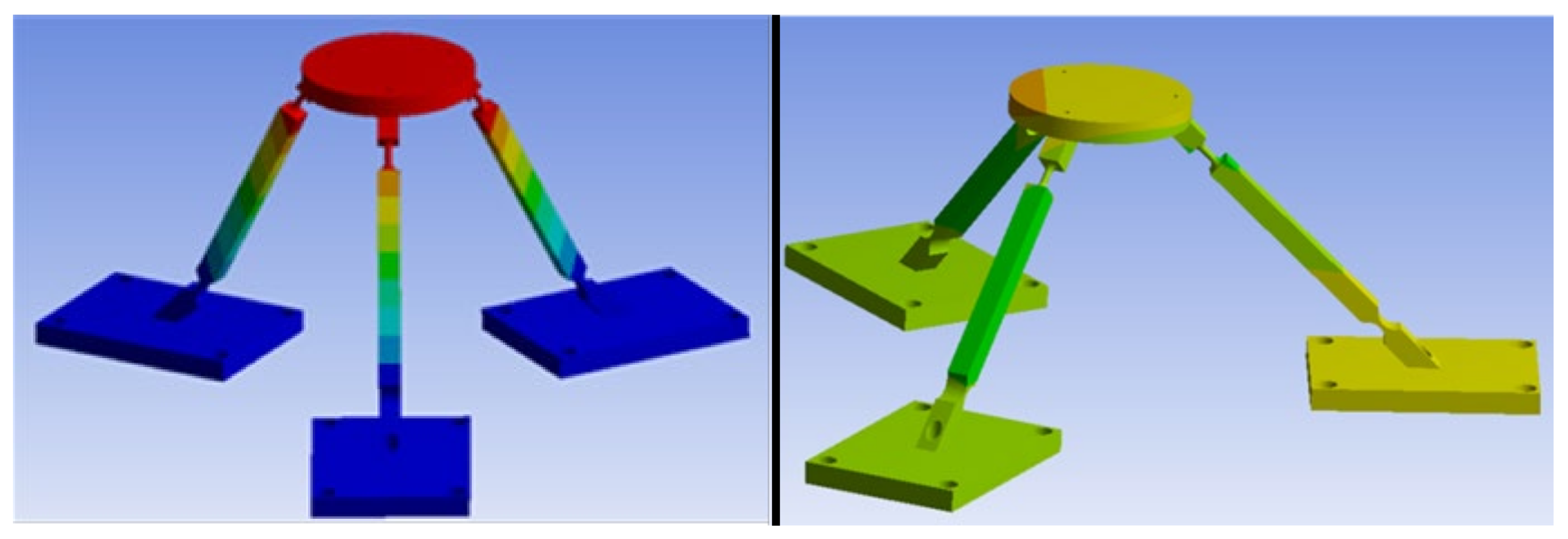
The 3PRS preliminary prototype here modeled was designed with the aim of providing Z motion of ±2 mm and tilting of ±1 degrees to molds for micro lenses during their milling process; see Figure 2. Its design and construction is presented in [24] and the dynamic modeling in [25]. There, the precision of the manipulator was tested when reaching fixed positions by measuring the position reached by the platform and the actuators with a coordinate-measuring machine, basing the modeling of the mechanism in a pseudo rigid body approach, as in [1]. In the present work, the mechatronic model developed to predict the performance of the system is presented. The mechatronic model integrates the dynamics of the compliant manipulator, actuators, and control. In this way, the influence on the manipulator performance of the control algorithm and its parameters and vice versa can be considered, providing a reliable estimation of the bandwidth of the manipulator, apart from validating a given selection of actuators and a control algorithm or its gains tuning. This kind of modeling is along the lines proposed by the guideline VDI 2206 for mechatronic design [26]. Data, such as the motor torque/force and motor position of platform position, can be affected by the control algorithm and the gain tuning, so this kind of approach is mandatory for a better estimation of the dynamic performance.
The dynamics of the compliant mechanism is modeled with a pseudo rigid body approach, that is, replacing the flexure hinges by conventional joints with springs to model the flexure stiffness [1]. This approach not only simplifies the dynamic analysis, but also allows using the dynamic model for a future optimization of the control algorithm. FEM models, although they can be more suitable for a thorough dynamic modelling, are not easy to implement in control algorithms [10]. In the following section, the details of the mechatronic model are shown. In Section 3, the tests performed to validate the mechatronic model are shown, and then discussed in Section 4. Conclusions are shown in Section 5.
2. Mechatronic Model and Hypotheses
The approach followed for the mechatronic modeling is based on decoupling the 3PRS compliant mechanism from the actuators, see Figure 3, in such a way that the forces required to move the manipulator are seen as if they were a disturbance from the perspective of the actuators. In this way, it is possible to decouple the modeling of the mechanism from the modeling of the actuators, which can be more detailed with several degrees of freedom if desired.
Hence, the mechatronic model follows these steps, as seen in Figure 4, assuming that a joint space control is going to be performed. First, the commanded displacement in workspace coordinates (ψc, θc, pzc) is introduced into the inverse kinematic problem to obtain the commanded joint space coordinates (s1c, s2c, s3c). Second, these are introduced into the dynamic model of the control and actuators, which models the cascaded position, velocity and current control loops as well as the actuators dynamics. As the force required to deform the compliant mechanism can be higher than in a conventional mechanism, it is advisable to model the stiffness of the actuator and its transmission chain, as it may happen that a given transmission is less rigid than the compliant mechanism itself. For that purpose, in the present work, a 2-degrees-of-freedom model with two inertias linked by a torsional spring and damper is proposed. As a result of this modeling, the position reached by the actuators is obtained, which is, third, fed into the direct kinematic problem to know the simulated position of the manipulator.
Fourth, to consider the dynamics of the compliant manipulator, the position reached is fed into the inverse dynamic problem of the manipulator. There, the main assumption is to consider the flexures as conventional joints with torsional springs, whose stiffness is considered constant inside the workspace of the manipulator, and it is calculated by FEM analysis [10]. The forces obtained (F1, F2, F3) are then fed back into the model of the actuators, where they act as if they were disturbances that the control must counteract to reach the desired position. This approach of decoupling actuators and control dynamics from the manipulator dynamics allows a more detailed modeling of the control or actuator, as is the case here with 2-degrees-of-freedom modeling in state-space.
In the following section, all the theoretical considerations to develop the mechatronic model of the compliant 3PRS are thoroughly shown, mainly, the kinematics and the dynamics of both the manipulator and the control and actuators.
3. Kinematics
The kinematic diagram of the 3PRS manipulator is shown in Figure 5. The mobile platform has the end effector in P. Three bars CiBi of equal length L connect the base and the mobile platform by means of an actuated prismatic joint P, a revolute joint R in Ci, and a spherical joint S in Bi. The angles αi between the bars and the fixed base are 45° in the default position. The Bi points are in a circumference of radius b with center in P. The origin of the linear actuators is located in Ai over a circumference of radius a and center in O. The actuators are inside three vertical planes at 120°, and their location is defined by the joint space coordinates si.
Two reference systems are defined. The fixed system XYZ has the origin in O, with the X-axis aligned with OA1, and the Z-axis is vertical. The XOY plane is horizontal at a height defined by the center of the compliant revolute joints. The mobile system UVW has the origin in P with the U-axis aligned with PB1 and the W-axis perpendicular to the mobile platform. It is also shifted in such a way that the UPV plane contains the center of the compliant spherical joints.
The platform position is defined by the workspace coordinates px, py, and pz that determine the position of P and three angles ψ, θ, and ϕ, which are the rotations around the X-, Y- and Z axes. This is a low mobility parallel mechanism with 3 degrees of freedom pz, ψ, and θ, and 3 parasitic motions, px, py and ϕ. The parasitic motions of this 3PRS mechanism are already presented in [24] and here, for completeness, we have included the formulation in Appendix A. In addition, the inverse kinematics problem to calculate the joint space coordinates si to reach a given position of the mobile platform in shown in Appendix B. The direct kinematics problem to determine the task space coordinates from the joint space ones is presented in Appendix C.
Finally, the rotation in the revolute and spherical joints is calculated to obtain the bending and torsional moments due to the deformation of the compliant joints represented there. The formulation is shown in Appendix D. The rotation in the compliant revolute joints is measured by the angle αi. The torsional rotation around the CiBi bars is measured by the angle βli, the bending rotation inside the vertical planes that contain the bar is determined by βmi, and the angle due to the bending in perpendicular direction to the vertical planes is βni.
3.1. Jacobians
For the resolution of the inverse dynamic problem, the Jacobians of the different elements of the manipulator are required.
3.1.1. Jacobian of the Mobile Platform
Closing the kinematic loop for each bar from O to Bi, both through P and Ai, the following equation is obtained:
The li0 unity vectors define the direction of the bars and si0 define the positive direction of the actuators. The derivative with respect to time is
where vp is the velocity of P, wp is the angular velocity of the mobile platform, and wi is the angular velocity of the bar i. Applying the dot product by li0,
and in matrix form,
where
On the other hand, due to the revolute joints, the motion of the bars is planar in a vertical plane whose normal vector is mi0. Those restrictions can be expressed as follows:
The derivative with respect to time is
In matrix form,
Grouping Equations (4) and (8),
Finally, the Jacobian of the mobile platform is obtained as follows:
3.1.2. Jacobian of the BiCi Bars
Calculating the dot product of Equation (2) and PBi and rearranging,
The angular velocity of the i-th bar wi can be posed as follows:
Substituting Equation (12) in Equation (11), introducing Equation (A20) and rearranging,
where
Substituting Equation (14) in Equation (13) and rearranging in matrix form, Jαi is the Jacobians that relate the angular velocity of the bars with the velocity of the actuators:
where
On the other hand, the position of the mass center of each bar is
Differentiating and rearranging,
In matrix form, and introducing the Jacobian of each bar as obtained in Equation (15) and the Kronecker delta,
Finally, the Jacobian of each i-th bar is calculated as
3.1.3. Jacobian of the Rotation of the Spherical Joints
To relate the first derivative of the rotations in the spherical joints with the velocity of the actuators, first, the platform angular velocity in Equation (28) is substituted by the following expression, which considers the relative motion of the platform with respect to each one of the bars.
Hence, the following nine equations result:
Applying the dot product by li0 and rearranging,
In matrix form, for the relative motion to one of the j-th bars,
In Equation (24), the relative velocity to the j-th bar in the XYZ reference system is the sum of the rotations around mj, nj and lj in the local reference system Sj, premultiplied by the corresponding rotation matrix Rj as defined in Equation (23).
Additionally, in Equation (24), the term dependent on the velocity of P can be expressed as in Equation (26) using Equation (36).
What is more, in Equation (24), the term dependent on the angular velocity of the j-th bar can be expressed as follows, substituting Equations (38) and (15).
Introducing Equations (25)–(27) in Equation (24), the desired Jacobian for the spherical joint of the j-th is obtained:
where the direct and inverse Jacobians are, respectively,
4. Dynamics
To solve the inverse dynamic problem of the manipulator, it is divided in n subsystems of open chain, where the Lagrange equations can be conveniently applied with respect to the local generalized coordinates, qn. The equations of motion of those elements are posed as a function of the generalized forces τn and the Lagrangian Ln, dependent on the kinetic energy Tn and the potential energy Vn.
If the n subsystems move as if they were assembled, the set of local generalized coordinates of all subsystems qN is a function of the global generalized coordinates of the assembled mechanism qs. Hence, their virtual displacements can be related through the corresponding Jacobian:
On the other hand, if all subsystems move as if they were assembled, the virtual work done during a generic motion must be the same as in the assembled mechanism; hence,
Therefore, the actuator forces needed to move the manipulator are obtained as
This is the so-called Principle of Energy Equivalence, which is applied to the 3PRS elements in the following subsections, being that qs = s = {s1 s2 s3}T and τs = { F1 F2 F3}T. This approach allows the direct and systematic obtainment of the forces on the manipulator, and it was partially developed in [11], where the moments due to the flexures’ deflection were considered external actions. Here, the complete formulation, including the proper modeling of the bending and torsional moments in the joints, is considered.
4.1. Mobile Platform
In the mobile platform subsystem, the following contributions to the Lagrangian will be considered: the one due to the translational motion with the total mass located in the center of mass, the one due to the rotational motion around the center of mass, and the elastic energy due to the deformation of the spherical joints.
The external forces acting on the mobile platform are also considered. If an external force fextm = {Fu Fv Fw}T is applied on a point D located as PDm = {du dv dw}T, the force and the moments on the manipulator in the fixed reference system XYZ are
4.1.1. Translational Dynamics
Considering the platform as a point mass located in the center of mass located in P, the Lagrangian can be expressed as
where Mplat is the mass of the mobile platform and g is the gravity. Applying the Lagrange equation, the equations of motion in matrix form are
To apply the Principle of Energy Equivalence, first the local generalized coordinates are replaced as a function of the global ones through the corresponding Jacobian in Equation (36). There, the Jacobian of the platform can be divided in a translational and a rotational part as
Hence, after derivation and substitution, Equation (36) becomes
Finally, the contribution of this motion to the dynamics of the assembled manipulator is obtained by premultiplying the transpose of the Jacobian:
4.1.2. Rotational Dynamics
To consider the dynamics of the rotation around the center of mass, the Boltzmann–Hamel equations are used. These equations allow a simpler resolution of the Lagrange equations, using the components of the angular velocity of the platform in the UVW mobile reference system as quasivelocities. The quasivelocities depend on the platform rotations ψ, θ, and ϕ and their derivatives as follows:
Equation (37) relates the angular velocity of the platform in the XYZ reference system with the global generalized coordinates of the mechanism through the Jacobian. Applying the inverse of the rotation matrix and substituting Equation (37) in Equation (40),
The Lagrangian due to this motion can be posed as a function of the kinetic energy obtained in the UVW system:
To differentiate the Lagrange equations with respect to the platform rotations, the Boltzmann–Hamel equations and the Lagrange equations make use of the quasivelocities as partial differentiations in order to avoid too complex operations:
where
Substituting in Equation (43),
To obtain the contribution of this motion to the global dynamics of the manipulator, first, Equation (41) is introduced to relate the angular velocity in UVW with the global generalized coordinates:
Then, premultiplication by the transpose of the Jq Jacobian is applied. In addition, as the external torque is already calculated in the XYW reference system, it is premultiplied by the platform Jacobian.
4.1.3. Contribution of the Elastic Energy in the Spherical Joints
The relative motion of the platform with respect to the bars results in the elastic deformation of the spherical joints, that must be taken into account. The Lagrangian presents here only a contribution from the potential energy
where
being that ksf and kst are the flexural and torsional stiffnesses of the spherical joints, and βi is the angles obtained in Equation (26). Having calculated the corresponding Jacobians in Equation (28), the contribution to the equation of motion can be posed directly as
4.2. Couplings between Actuators and 3PRS Manipulator
The local generalized coordinates of the manipulator coupling with the actuators are the same as the global generalized coordinates, si, where Fi is the forces that the actuators must do. The Lagrangian takes into account the kinetic energy of the couplings and the elastic energy due to the deflection of the compliant revolute joints, where Mi is the mass of the couplings and kr is the flexural stiffness of the joints. Being that α0 is the α angle in the default position with no deformation,
Hence, applying the Lagrange equations, and introducing the transpose of the Jacobian obtained in Equation (15), the contribution to the global dynamics in matrix form is obtained as in Equation (52).
4.3. BiCi Bars
The local generalized coordinates selected for the bars are the position of the center of mass, xGi, yGi, and zGi, and their angle αi. Being that Mb is the mass of the bars and IbG is their inertia moment in that point, their Lagrangian is
Applying the Lagrange equation to each generalized coordinate of the bars and grouping in matrix form,
where the Jacobian that relates the rotations in the spherical joints with the local generalized coordinates of the bar is
Hence, in matrix form, the equation of motion of each i-th bar subsystem is
Introducing the Jacobian in Equation (20) to apply the Principle of Energy Equivalence,
Substituting in Equation (56) and premultiplying by the transpose of the Jacobian of the bar Jbi, the contribution of each bar to the dynamics of the manipulator is
where is obtained in Equation (28).
4.4. Dynamic Model of the Whole Mechanism
Taking into account all the contributions, the equation of motion of the 3PRS compliant manipulator will be
4.5. Dynamic Model of the Control and Actuators
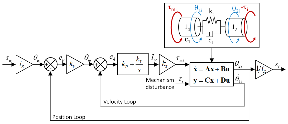
The manipulator is controlled using a joint-space control approach, where the workspace position commands are fed through the inverse kinematic problem to obtain the position commands sic in the joint space. Then, the position control is done using a cascaded control of position, velocity and current that is modelled in Simulink following the scheme of Figure 6. A proportional controller (kV) is used in the position loop, whereas a proportional–integral (kP, kI) control is used in the velocity loops. As the current loop runs at a lower loop cycle, the conversion from current to torque is assumed to be immediate through the motor torque constant kT, so the current loop is simplified in this way. The transmission ratio of the actuators is iR.
In the model represented in Figure 6, the dynamics of the actuators are represented by a state-space model that relates, respectively, the motor torque and the mechanism disturbance with the motor velocity and the motor position. The state-space model is calculated, modeling the actuator transmission with a 2 degrees of freedom model with two inertias coupled by a torsional spring and damper to consider the flexibility of the transmission.
Hence, the terms of the state-space model are as follows:
5. Experimental Validation
A prototype is developed to test the validity of the mechatronic model developed. All the elements of the compliant manipulator are built in Aluminum 7075-T6, as seen in Figure 7. The actuators are linear belt drives from Igus of 70 mm/rev, model ZLW-1040-02-S-100 coupled to RE-40 Maxon DC servomotors with GP-32 14:1 reductor. The control system is implemented in a NI-PXIe 1062, which works in real time with a position loop cycle time of 5 ms. The only sensors are the encoders of the Maxon motors and the torque measurement from the motors’ drives. Although the error in the transmission is not compensated by the control, the mechatronic model has considered this fact in the control model, so it should be predicted.
A compilation of all the dimensional parameters and dynamic parameters of the compliant 3PRS as well as the control parameters is shown in Table 1. The stiffness of the flexure hinges of the revolute and spherical joints was calculated by FEM in [24].
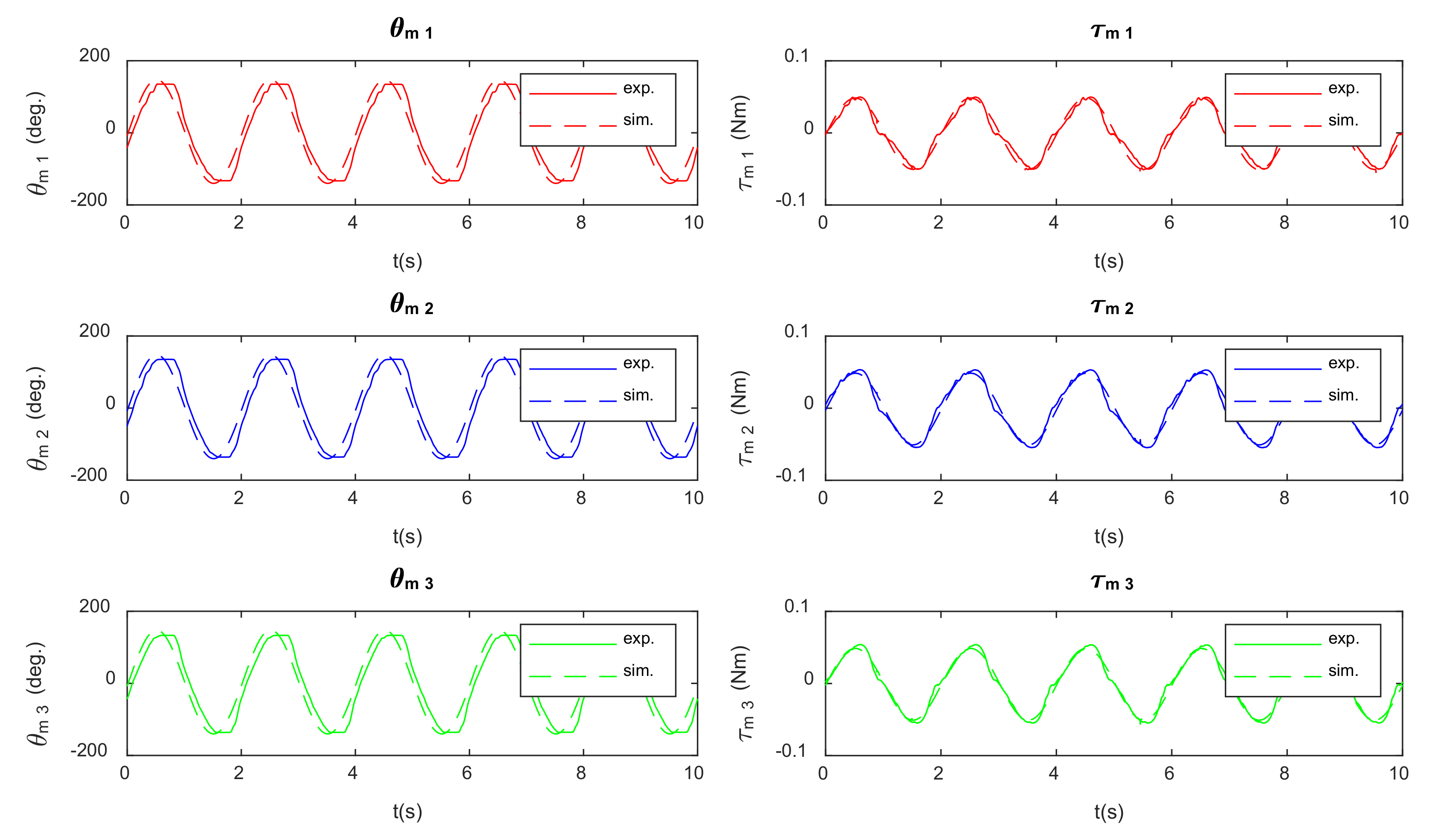
To validate the mechatronic model with the prototype, the simulated motor position and torque are compared with the corresponding signals measured during the tests. Two examples of the motions tested are shown here. First, the mobile platform performs a translation in Z direction with a sine profile with an amplitude of 2 mm and a frequency of 0.5 Hz; see Figure 8. Then, the same motion is performed but with a phase shift between actuators of 120°, see Figure 9, to generate a variable tilting in the table. To avoid problems due to fatigue and cracks in the flexure hinges, a new set of bars is used.
6. Discussion
As it can be seen in Figure 8 and Figure 9, the results obtained in both motions by the simulation resemble the measurements, taking into account all the simplifications made and the fact that the dynamic parameters used are the theoretical ones, that is, they are not experimentally verified to evaluate the degree of accuracy of the simulation used as a design tool previous to the manufacturing of the prototype. There is a little delay between the experimental and simulated signals due to the difficulty in time aligning the initial moment of the motion. Additionally, the error is higher in the rotation motion of Figure 9, which is a more complex motion than the translation in Z of the Figure 8, where all the actuators move in unison. There are several sources for these errors, mainly manufacture errors in the prototype, the possible difference between the real dynamic parameters and the estimated ones, the modeling errors, and the appearance of disturbances as friction and nonlinearities in the linear belt drives.
What is more, the profile of the torque signals in both figures suggest that there are nonlinearities in the system. Part of it is due to the dry friction in the actuators. However, after examining separately the manipulator and the actuators with the linear belt drives, the cause of that nonlinearity lies mainly on the linear belt drives, where the belt is not stiff enough to properly actuate the compliant 3PRS. The belt is preloaded and works under traction but, under higher forces, it is further deformed. As the length of belt under traction is not the same when the drive moves in positive and negative directions, its stiffness also changes depending on the direction of the motion. In addition, the top and bottom of the angular position in the motors are flat, which could be related to this behavior of the belt drives.
7. Conclusions
An integrated approach for the mechatronic modeling of a compliant 3PRS parallel manipulator is presented. This approach considers the kinematics and dynamics of the compliant mechanism, the dynamics of the actuators and the dynamics of the control algorithm. The model can be used to validate the design of the compliant manipulator, and to evaluate and select the best control algorithm or set of actuators by simulating the response to a given motion profile.
The model is based on decoupling the dynamics of the manipulator and the actuators, so that the input force on the manipulator is considered by the actuators as if it was a disturbance that should be counteracted by the control.
For the dynamic modeling of the manipulator, the flexures are simplified using a pseudo rigid body approach, considering them as conventional joints with torsional springs that model the bending or torsional moments. This simplifies the dynamic modeling, avoiding the use of FEM, and the problem becomes more parameterizable. To solve the inverse dynamic problem, the Principle of Energy Equivalence is used, which allows the direct obtainment of the input forces required and also decouples the contribution to the global dynamics of each part of the manipulator.
Regarding the dynamics of the control and the actuator, the control algorithm is simulated, modeling the actuators with a 2-degrees-of-freedom model that allows considering their stiffness, which can be relevant when trying to deform the compliant mechanism.
The model is validated with a prototype developed, proving that the predictions made are similar to the experimental tests. Nevertheless, there are still some deviations that can be due to all the simplifications made, but mainly seems to be due to the unexpected nonlinear behavior of the linear belt drives used for the prismatic joints.
Author Contributions
Conceptualization, F.J.C., A.R. and O.A.; methodology, F.J.C. and A.R.; software, A.R., S.H. and M.D.; validation, A.R., F.J.C. and M.D.; formal analysis, O.A.; investigation, A.R.; resources, S.H.; data curation, A.R.; writing—original draft preparation, F.J.C.; writing—review and editing, A.R., S.H. and M.D.; visualization, F.J.C.; supervision, O.A.; project administration, F.J.C.; funding acquisition, F.J.C. All authors have read and agreed to the published version of the manuscript.
Funding
Authors would like to thank the Ministerio de Ciencia e Innovación of the Spanish government for funding the project PID2019-105262RB-I00.
Institutional Review Board Statement
Not applicable.
Informed Consent Statement
Not applicable.
Data Availability Statement
Not applicable.
Conflicts of Interest
The authors declare no conflict of interest.
Appendix A. Parasitic Motions
According to Figure 4, the position of the end effector point P is
The position of the spherical joints Bi in the mobile reference system is
To represent those vectors in the fixed reference system XYZ, the rotation matrix that relates UVW and XYZ is defined as
where u, v and w are the unity vectors that define the axis of the UVW reference system, and c and s refer to cosine and sine, respectively. Hence, the position of each spherical joint in the fixed reference system XYZ is
Considering that the revolute joints in Ci restrict the motion of the spherical joints to a plane defined by the linear actuators OAi and the manipulator bars CiBi, so the following conditions must be met:
Substituting the equations of restriction in Equation (A5) and the terms of the rotation matrix in Equation (A3) into Equation (A4), the expressions of the parasitic motions of the 3PRS manipulator are obtained, which are a rotation around the Z-axis and two translations in X and Y:
Appendix B. Inverse Kinematic Problem
First, the following kinematic relation defines the position of the spherical joints with respect to the origin of the actuators:
The origin of the actuators in the XYZ system is
In addition, the vectors CiBi that locate the spherical joints with respect to the prismatic joints can be written as in Equation (A9). Their modulus is the length L of the bars:
The unit vectors si0 define the positive direction of the actuators motion:
The li0 unity vector defines the direction of the bars and is calculated as
Rearranging and squaring Equation (A10), a quadratic equation is obtained.
Solving it, the inverse kinematic problem, that is, the position of the actuators si, is calculated.
Appendix C. Direct Kinematic Problem
Calculating the vectors that define the position of the spherical joints with respect to the revolute joints in Ci,
In addition, imposing the condition of fixed length L of the CiBi bars in the following equations,
where the OCi vectors are
Substituting Equation (A16) and Equation (A4) in Equation (A15) for each i bar, the following nonlinear equations are obtained, which allow calculating the position pz and the angles Ψ, and θ of rotation around the X and Y axes.
Appendix D. Passive Coordinates
The rotation in the compliant revolute joints is measured by the angle αi between the CiBi bars and the XY plane can be calculated as
The rotation of the joint is then calculated as the difference between αi and the default angle 45°.
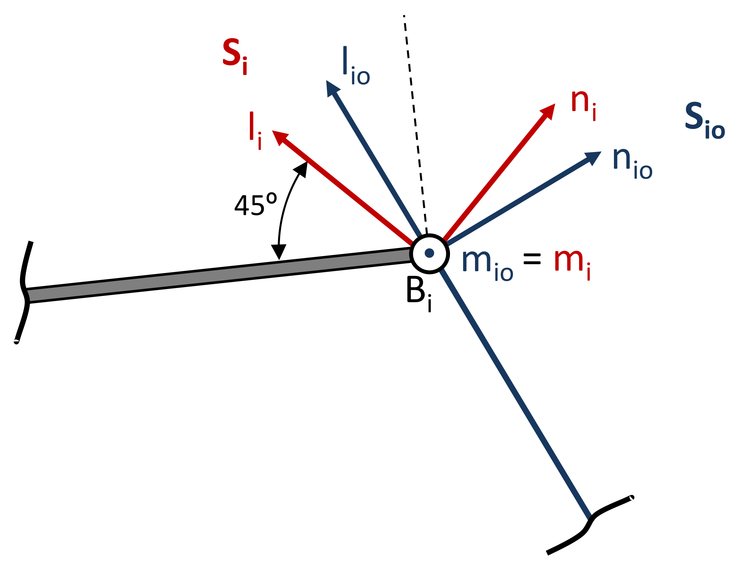
To calculate the rotations in the spherical joints, angles βmi, βni and βli, the relative rotation matrix between the MNL reference systems in Figure A1 must be obtained. Two reference systems MNL are used with the origin in the Bi spherical joints. The first one, Si0, is fixed to the mobile platform, and the second one, Si, is fixed to the CiBi bars, as it is seen in Figure A1. Rotations around the axis defined by unity vectors mi and ni, βmi and βni, refers to the deflections in the spherical joint in those directions, and rotation around the axis defined by li, βli, measures the torsional deformation of the joint.
Figure A1.
Reference systems in the spherical joints.

First, regarding the unit vectors of the Si0 system in the fixed reference system XYZ is, lio is already shown in Equation (A11). Additionally, mio is the unit vectors orthogonal to the vertical planes that contain the bars, defined as
Unity vectors ni0 are calculated from the following cross product:
Hence, the rotation matrix Ri0 of the reference system Si0 is
Doing the same for the Si reference system, unit vectors mi, ni and li in the UVW system are defined as
In the fixed reference system XYZ, those vectors are expressed premultiplying with the rotation matrix of the mobile platform:
Finally, the rotation matrix Ri-i0 between reference systems Si0 and Si is obtained as
On the other hand, Ri-i0 can be developed as a function of the three consecutive rotations around m, n and l axis. The resultant matrix is
Equaling terms in Equations (A24) and (A25), the following rotations for the spherical joints are obtained:
References
- Howell, L. Compliant Mechanisms; Wiley: New York, NY, USA, 2001. [Google Scholar]
- Bryson, C.E.; Rucker, D.C. Toward Parallel Continuum Manipulators. In Proceedings of the 2014 IEEE International Conference on Robotics and Automation (ICRA), Hong Kong, China, 31 May–7 June 2014; pp. 778–785. [Google Scholar]
- Grioli, G.; Wolf, S.; Garabini, M.; Burdet, E. Variable stiffness actuators: The user’s point of view. Int. J. Robot. Res. 2015, 34, 727–743. [Google Scholar] [CrossRef] [Green Version]
- Stoeffler, C.; Kumar, S.; Müller, A. A Comparative Study on 2-DOF Variable Stiffness Mechanisms. In Springer Proceedings in Advanced Robotics; Lenarčič, J., Siciliano, B., Eds.; Advances in Robot Kinematics 2020. ARK 2020; Springer: Cham, Germany, 2021; p. 15. [Google Scholar]
- Lemerle, S.; Catalano, M.G.; Bicchi, A.; Grioli, G. A Configurable Architecture for Two Degree-of-Freedom Variable Stiffness Actuators to Match the Compliant Behavior of Human Joints. Front. Robot. AI 2021, 8, 10. [Google Scholar] [CrossRef] [PubMed]
- Choi, Y.; Kim, J. A millimeter-range flexure-based nano-positioning stage using a self-guided displacement amplification mechanism. Mech. Mach. Theory 2012, 50, 109–120. [Google Scholar]
- Choi, H.; Han Ch Wang, W. 2-DOF Kinematic XY stage design based on flexure element. In Proceedings of the IEEE International Conference on Mechatronics and Automation, Beijing, China, 7–10 August 2011. [Google Scholar]
- Aphale, S.; Moheimani, S.; Yong, Y. Design, Identification, and Control of a Flexure-Based XY Stage for Fast Nanoscale Positioning. IEEE Trans. Nanotechnol. 2009, 8, 46–54. [Google Scholar]
- Ahn, D.; Chun, B.; Gweon, D.; Kim, H. Development and optimization of a novel 3-DOF precision flexure stage. In Proceedings of the IEEE International Conference on Nanotechnology Joint Symposium with Nano Korea, Kintex, Korea, 17–20 August 2010. [Google Scholar]
- Gao, F.; Ge, Q.; Yue, Y.; Zhao, X. Relationship among input-force, payload, stiffness and displacement of a 3-DOF perpendicular parallel micro-manipulator. Mech. Mach. Theory 2010, 45, 756–771. [Google Scholar]
- Kenton, B.; Leang, K. Design and Control of a Three-Axis Serial-Kinematic High-Bandwidth Nanopositioner. IEEE/ASME Trans. Mechatron. 2012, 17, 356–369. [Google Scholar] [CrossRef]
- Hao, G.; Kong, X. Design and Modeling of a Large-Range Modular XYZ Compliant Parallel Manipulator Using Identical Spatial Modules. J. Mech. Robot. 2012, 4, 021009. [Google Scholar] [CrossRef]
- Lobontiu, N. Compliant Mechanisms: Design of Flexure Hinges, 1st ed.; CRC Press: Boca Raton, FL, USA, 2002. [Google Scholar] [CrossRef]
- Yong, Y.K.; Lu, T.F.; Handley, D.C. Review of circular flexure hinge design equations and derivation of empirical formulations. Precis. Eng. 2008, 32, 63–70. [Google Scholar] [CrossRef]
- Yong, Y.K.; Lu, T.F. Comparison of circular flexure hinge design equations and the derivation of empirical stiffness formulations. In Proceedings of the IEE/ASME International Conference on Advanced Intelligent Mechatronics, Singapore, 14–17 July 2009. [Google Scholar]
- Schoenen, D.; Hüsing, M.; Corves, B. Dynamic Analysis of a Fatigue Test Bench for High Precision Flexure Hinges. In Microactuators and Micromechanisms; Zentner, L., Corves, B., Jensen, B., Lovasz, E.C., Eds.; Mechanisms and Machine Science; Springer: Cham, Germany, 2017; Volume 45. [Google Scholar] [CrossRef]
- Liu, C.; Bi, Z.; Ran, J.; Gu, J.; Wang, X.; Zhang, C. Modelling and verification of fatigue damage for compliant mechanisms. Robotica 2019, 37, 1–17. [Google Scholar] [CrossRef]
- Carretero, J.A.; Podhorodeski, P.; Nahon, M.A.; Gosselin, C.M. Kinematic analysis and optimization of a new three degree of freedom spatial parallel manipulator. J. Mech. Des. 2000, 122, 17–24. [Google Scholar] [CrossRef]
- Carretero, J.A.; Nahon, M.A.; Podhorodeski, R.P. Workspace analysis and optimization of a novel 3-DOF parallel manipulator. Int. J. Robot. Autom. 2000, 15, 178–188. [Google Scholar]
- Li, Y.; Xu, Q. Kinematic analysis of a 3-PRS parallel manipulator. Robot. Comput.-Integr. Manuf. 2007, 23, 395–408. [Google Scholar] [CrossRef]
- Li, Y.; Xu, Q. Kinematics and inverse dynamics analysis for a general 3-PRS spatial parallel mechanism. Robotica 2005, 23, 219–229. [Google Scholar] [CrossRef] [Green Version]
- Tsai, M.S.; Yuan, W.-H. Inverse dynamics analysis for a 3-PRS parallel mechanism based on a special decomposition of the reaction forces. Mech. Mach. Theory 2010, 45, 1491–1508. [Google Scholar] [CrossRef]
- Tourajizadeh, H.; Gholami, O. Optimal Control and Path Planning of a 3PRS Robot Using Indirect Variation Algorithm. Robotica 2020, 38, 903–924. [Google Scholar] [CrossRef]
- Ruiz, A.; Campa, F.J.; Roldán-Paraponiaris, C.; Altuzarra, O.; Pinto, C. Experimental validation of the kinematic design of 3-PRS compliant parallel mechanisms. Mechatronics 2019, 39, 77–88. [Google Scholar] [CrossRef]
- Ruiz, A.; Campa, F.J.; Roldán-Paraponiaris, C.; Altuzarra, O. Dynamic Model of a Compliant 3PRS Parallel Mechanism for Micromilling. In Proceedings of the 4th Conference on Microactuators and Micromechanisms, Ilmenau, Germany, 5–7 October 2016; Zentner, L., Corves, B., Jensen, B., Lovasz, E.C., Eds.; Springer: Berlin/Heidelberg, Germany, 2016. [Google Scholar]
- Gausemeier, J.; Moehringer, S. VDI 2206-A New Guideline for the Design of Mechatronic Systems. IFAC Proc. Vol. 2002, 35, 785–790. [Google Scholar] [CrossRef]
Figure 1.
(Top) 3PRS compliant parallel manipulator developed. (Bottom) Revolute and spherical joints used.
Figure 1.
(Top) 3PRS compliant parallel manipulator developed. (Bottom) Revolute and spherical joints used.

Figure 2.
FEM simulations: (Left) Maximum position in Z direction. (Right) Maximum tilting around Y axis.
Figure 2.
FEM simulations: (Left) Maximum position in Z direction. (Right) Maximum tilting around Y axis.

Figure 3.
Decoupling of the compliant mechanism and actuators.

Figure 4.
Mechatronic model of the compliant 3PRS.

Figure 5.
Schematic diagram of the 3PRS kinematics.

Figure 6.
Modeling of the control and actuators dynamics.

Figure 7.
Experimental setup.

Figure 8.
Experimental vs. simulated signals: (Left) Angular position of the motors. (Right) Motor torque.
Figure 8.
Experimental vs. simulated signals: (Left) Angular position of the motors. (Right) Motor torque.

Figure 9.
Experimental vs. simulated signals: (Left) Angular position of the motors. (Right) Motor torque.
Figure 9.
Experimental vs. simulated signals: (Left) Angular position of the motors. (Right) Motor torque.


Table 1.
Parameters of the compliant 3PRS: dimensions, dynamic parameters, control parameters.
| Parameter | Value | Units |
|---|---|---|
| a | 125.137 | mm |
| b | 47.61 | mm |
| L | 109.215 | mm |
| Mb | 0.028 | kg |
| IbG | 2.36 × 10⁻⁵ | kgm2 |
| Mplat | 0.153 | kg |
| α0 | 45 | deg. |
| Iplatu | 6.834 × 10⁻⁵ | kgm2 |
| Iplatv | 6.834 × 10⁻⁵ | kgm2 |
| Iplatw | 1.309 × 10⁻⁵ | kgm2 |
| Mi | 0.204 | kg |
| kr | 98.37 | Nm/rad |
| ksf | 32.665 | Nm/rad |
| kst | 24.46 | Nm/rad |
| iR | 2 × π × 14/0.07 | - |
| kV | 65 | 1/s |
| kP | 1 | As |
| kI | 8 | A |
| kT | 0.0302 | Nm/A |
| J1 | 1.423 × 10⁻⁴ | kgm2 |
| J2 | 4.817 × 10⁻⁸ | kgm2 |
| ct | 1.085 × 10⁻⁵ | Ns/m |
| c1 | 0.003 | Ns/m |
Publisher’s Note: MDPI stays neutral with regard to jurisdictional claims in published maps and institutional affiliations. |
© 2021 by the authors. Licensee MDPI, Basel, Switzerland. This article is an open access article distributed under the terms and conditions of the Creative Commons Attribution (CC BY) license (https://creativecommons.org/licenses/by/4.0/).
Share and Cite
MDPI and ACS Style
Ruiz, A.; Campa, F.J.; Altuzarra, O.; Herrero, S.; Diez, M. Mechatronic Model of a Compliant 3PRS Parallel Manipulator. Robotics 2022, 11, 4. https://0-doi-org.brum.beds.ac.uk/10.3390/robotics11010004
AMA Style
Ruiz A, Campa FJ, Altuzarra O, Herrero S, Diez M. Mechatronic Model of a Compliant 3PRS Parallel Manipulator. Robotics. 2022; 11(1):4. https://0-doi-org.brum.beds.ac.uk/10.3390/robotics11010004
Chicago/Turabian StyleRuiz, Antonio, Francisco J. Campa, Oscar Altuzarra, Saioa Herrero, and Mikel Diez. 2022. "Mechatronic Model of a Compliant 3PRS Parallel Manipulator" Robotics 11, no. 1: 4. https://0-doi-org.brum.beds.ac.uk/10.3390/robotics11010004
Note that from the first issue of 2016, this journal uses article numbers instead of page numbers. See further details here.